Embed Size (px)
Citation preview
MAXIMUM POWER POINT TRACKING ALGORITHM FOR
PHOTOVOLTAIC HOME POWER SUPPLY
by
CEDRICK LUPANGU NKASHAMA
Dissertation
Submitted in partial fulfillment for the requirements of the Degree
Master of Science in Electrical Engineering
Faculty of Engineering
University of KwaZulu-Natal, Durban
Supervisor: Dr Akshay Kumar Saha
April, 2011
ii
Declaration
I, Cedrick Lupangu Nkashama, declare that:
(i) The research reported in this dissertation/thesis, except where otherwise indicated, is my original work.
(ii) This dissertation/thesis has not been submitted for any degree or examination at any other university.
(iii) This dissertation/thesis does not contain other persons’ data, pictures, graphs or other information, unless specifically acknowledged as being sourced from other persons.
(iv) This dissertation/thesis does not contain other persons’ writing, unless specifically acknowledged as being sourced from other researchers. Where other written sources have been quoted, then:
a) their words have been re-written but the general information attributed to them has been referenced;
b) where their exact words have been used, their writing has been placed inside quotation marks, and referenced.
(v) Where I have reproduced a publication of which I am an author, co-author or editor, I have indicated in detail which part of the publication was actually written by myself alone and have fully referenced such publications.
(vi) This dissertation/thesis does not contain text, graphics or tables copied and pasted from the Internet, unless specifically acknowledged, and the source being detailed in the dissertation/thesis and in the References sections.
……………………… Cedrick Lupangu 29 April 2011 Durban, South Africa

iii
Acknowledgements
Special thanks to my lord and saviour Jesus-Christ for your support and comfort during difficult times
and the trials I passed through to complete this dissertation. You have been a real friend to me. May
your name be blessed!
I gratefully acknowledge the advice, guidance and encouragement received from my supervisor,
Dr A K Saha, from the School of Electrical, Electronic and Computer Engineering at the University of
KwaZulu-Natal (UKZN) during the completion of my dissertation.
I would also express my sincere gratitude to the High Voltage Direct Current (HVDC) centre in the
School of Electrical, Electronic and Computer Engineering at UKZN for their support and the
opportunity they gave me to further my studies in the field of Power and Energy Systems.
This work is dedicated to Sandrine, my wife, and Joyce and Claire, our two daughters, Dan, our new
baby boy, and our parents for their patience, love, understanding and support through prayers during
the period of my studies at UKZN.

iv
Abstract
Solar photovoltaic (PV) systems are distributed energy sources that are an environmentally friendly
and renewable source of energy. However, solar PV power fluctuates due to variations in radiation
and temperature levels. Furthermore, when the solar panel is directly connected to the load, the power
that is delivered is not optimal. A maximum peak power point tracker is therefore necessary for
maximum efficiency.
A complete PV system equipped maximum power point tracking (MPPT) system includes a solar
panel, MPPT algorithm, and a DC-DC converter topology. Each subsystem is modeled and simulated
in a Matlab/Simulink environment; then the whole PV system is combined with the battery load to
assess the overall performance when subjected to varying weather conditions.
A PV panel model of moderate complexity based on the Shockley diode equation is used to predict
the electrical characteristics of the cell with regard to changes in the atmospheric parameter of
irradiance and temperature.
In this dissertation, five MPPT algorithms are written in Matlab m-files and investigated via
simulations. The standard Perturb and Observe (PO) algorithm along with its two improved versions
and the conventional Incremental Conductance (IC) algorithm, also with its two-stage improved
version, are assessed under different atmospheric operating conditions. An efficient two-mode MPPT
algorithm combining the incremental conductance and the modified constant voltage methods is
selected from the five ones as the best model, because it provides the highest tracking efficiencies in
both sunny and cloudy weather conditions when compared to other MPPT algorithms.
A DC-DC converter topology and interface study between the panel and the battery load is performed.
This includes the steady state and dynamic analysis of buck and boost converters and allows the
researcher to choose the appropriate chopper for the current PV system. Frequency responses using
the state space averaged model are obtained for both converters. They are displayed with the help of
Bode and root locus methods based on their respective transfer functions. Following the simulated
results displayed in Matlab environment for both choppers, an appropriate converter is selected and
implemented in the present PV system. The chosen chopper is then modeled using the Simulink
Power Systems toolbox and validates the design specifications.
The simulated results of the complete PV system show that the performances of the PV panel using
the improved two-stage MPPT algorithm provides better steady state and fast transient characteristics
when compared with the conventional incremental conductance method. It yields not only a reduction
in convergence time to track the maximum power point MPP, but also a significant reduction in
power fluctuations around the MPP when subjected to slow and rapid solar irradiance changes.

v
Table of contents
Declaration ........................................................................................................................................ ii
Acknowledgements ................................................................................................................ iii
Abstract ................................................................................................................................. ii
Table of contents…………………………………………………………………………...… v
List of Figures ...................................................................................................................... viii
List of Tables ......................................................................................................................... xi
List of Abbreviations ............................................................................................................. xii
List of Symbols .................................................................................................................... xiii
Chapter 1: INTRODUCTION ................................................................................................ 1
1.1 Photovoltaic systems .......................................................................................................... 1
1.2 Background and Motivation ................................................................................................ 2
1.3 Stand-alone Photovoltaic Simulation System Used ................................................................. 3
1.4 Objectives, Methodology and Scope of the Study ................................................................... 4
1.5 Outline of the thesis ............................................................................................................ 6
Chapter 2: LITERATURE SURVEY ................................................................................ 7
2.1 Introduction ....................................................................................................................... 7
2.2 Performance criteria of MPPT control algorithms .................................................................. 9
2.2.1 Dynamic Response .......................................................................................................... 9
2.2.2 Steady state error ............................................................................................................. 9
2.2.3 Tracking Efficiency ....................................................................................................... 10
2.3 MPPT control algorithms classification ............................................................................... 10
2.4 Simple Panel-load matching .............................................................................................. 11
2.5 Semi-dynamic load matching ............................................................................................. 11
2.6 Voltage feedback methods................................................................................................. 12
2.6.1 Voltage feedback with fixed reference voltage .................................................................. 12
2.6.2 Voltage feedback with varying reference voltage by measurement of Voc ............................ 12
2.6.3 Pilot cell /reference module measurement approach ........................................................... 14
2.7 Power feedback control methods ........................................................................................ 15
2.7.1Perturb and Observe Control Algorithm ............................................................................ 16
2.7.1.1. Working Principle ...................................................................................................... 16
vi
2.7.1.2. Analysis of the PO algorithm ....................................................................................... 18
2.7.2 Incremental Conductance Control Algorithm .................................................................... 20
2.7.2.1 Working Principle ....................................................................................................... 20
2.7.2.2. Analysis of the IC algorithm ........................................................................................ 22
2.7.3 Block diagram of the MPPT control system ...................................................................... 23
2.8 Optimization solutions of MPPT control methods. ............................................................... 24
2.9. Conclusion ..................................................................................................................... 29
Chapter 3: PHOTOVOLTAIC MODELS ....................................................................... 31
3.1. Introduction .................................................................................................................... 31
3.2. Mathematical Model of PV cell ......................................................................................... 31
3.2.1 Simple PV cell model .................................................................................................... 31
3.2.2 Double exponential diode model ..................................................................................... 33
3.2.3 Single appropriate diode model ....................................................................................... 34
3.2.3.1 Matlab PV Cell model ................................................................................................. 35
3.2.3.2 Simulink PV Model .................................................................................................... 37
3.3 PV Simulated Results ....................................................................................................... 40
3.4 Conclusion and Discussion ................................................................................................ 41
Chapter 4: MAXIMUM POWER POINT TRACKING ALGORITHM MODELS ... 44
4.0 Introduction ..................................................................................................................... 44
4.1 Perturb and Observe (PO) Algorithm .................................................................................. 46
4.2 Perturb and Observe modified version 1(MPO) Algorithm .................................................... 48
4.3 Perturb and Observe modified version 2 or EPP Algorithm ................................................... 50
4.4 Incremental Conductance (IC) Algorithm ............................................................................ 53
4.5 Two-stage combined CV and IC Algorithm ......................................................................... 56
4.6 Average Output Power and Tracking Efficiency of MPPT Algorithms .................................... 59
4.7 Discussion and Analysis ................................................................................................... 60
Chapter 5: DC-DC CONVERTER TOPOLOGY AND INTERFACE ANALYSIS ...... 60
5.1 Switch-Mode Converter Theory ......................................................................................... 60
5.2 The Buck DC-DC Converter ............................................................................................. 63
5.2.1 Steady-state analysis ...................................................................................................... 63
5.2.2 Dynamic analysis .......................................................................................................... 68
5.3 The Boost DC-DC Converter ............................................................................................. 69

vii
5.3.1 Steady-state analysis ...................................................................................................... 68
5.3.2 Dynamic analysis .......................................................................................................... 73
5.4 Converter Topology Analysis and Comparison .................................................................... 74
5.4.1 Component Comparison ................................................................................................. 75
5.4.2 Modeling Comparison .................................................................................................... 80
5.5 Modeling and Simulation .................................................................................................. 84
Chapter 6: SYSTEM SIMULATION AND PERFORMANCE ANALYSIS .................. 86
6.1 Complete Simulink PV system........................................................................................... 86
6.2 Performance analysis ........................................................................................................ 94
6.3 Conclusion…………………………………………………………………………...…...94
Chapter 7: CONCLUSIONS AND FUTURE RESEARCH ............................................ 96
7.1 Conclusions ..................................................................................................................... 96
7.2 Future research ................................................................................................................ 98
Bibliography .................................................................................................................... 100
APPENDIX A..................................................................................................................... 104
APPENDIX B ..................................................................................................................... 111
APPENDIX C ..................................................................................................................... 129
APPENDIX D..................................................................................................................... 130
viii
List of figures
Figure 1-1: Applications of photovoltaic systems .................................................................. 2
Figure 1-2: Schematic diagram of PV simulation system used ............................................... 3
Figure 2-1: Intersection of I-V curve and load resistance variations ....................................... 6
Figure 2-2: I-V curves (a) irradiance variation (b) temperature variation ............................... 7
Figure 2-3: P-V curves (a) irradiance variation (b) temperature variation .............................. 7
Figure 2-4: Block diagram of MPPT method ......................................................................... 8
Figure 2-5:Schematic block diagram of the experimental semi-dynamic load matching……………..10
Figure 2-6: Voltage feedback MPPT methods with constant voltage reference .................... 11
Figure 2-7: Block diagram of the voltage feedback with adjustable reference……………………….12
Figure 2-8: Constant Voltage flowchart algorithm ............................................................... 13
Figure 2-9: Block diagram of pilot cell/reference module MPPT control system…………………...13
Figure 2-10: Characteristic of PV panel power curve........................................................... 16
Figure 2-11: Flowchart of the Perturb and Observe Algorithm……………………………………….17
Figure 2-12: Flowchart of the Incremental Conductance Algorithm………………………………….20
Figure 2-13: Block diagram of MPPT with direct control method........................................ 22
Figure 2-14: Block diagram of MPPT with PI compensator ................................................. 22
Figure 3-1: Equivalent circuit of a simple PV cell...................................................................31
Figure 3-2: Diagram showing short-circuit and open-circuit conditions…………………..……….…31
Figure 3-3: Equivalent circuit of two-diode solar cell model………………………..…..…..…….….33
Figure 3-4: Equivalent circuit of one diode solar cell………………………….………………….….34
Figure 3-5: Block diagram of Simulink PV model……………………………………….…………...38
Figure 3-6: Matlab I-V curves with variation……………………………………………………..…..39
Figure 3-7: Matlab I-V curves with T variation……………………………………...............39
Figure 3-8: Matlab P-V curves with T variation……………………….……………………………..40
Figure 3-9: Matlab P-V curves with G variation……………….…………….……………...40
Figure 3-10: Matlab I-V curves with Res variation……………………..…………………………….40
Figure 3-11: I-V curve of PV Simulink model…………………….………………...............41
Figure 3-12: P-V curve of PV Simulink model……………………………………................41
Figure 4-1: Measurement of cloudy and sunny irradiation in Upington, South Africa, 1966……...…44
Figure 4-2: Flowchart of “Perturb and Observe” algorithm .................................................. 45
Figure 4-3: MPPT capability of PO algorithm for a sunny day……………………………………….46
Figure 4-4: MPPT capability of PO algorithm for a cloudy day ........................................... 46
ix
Figure 4-5: Flowchart of PO Modified version 1(or MPO) algorithm…………………………..…....47
Figure 4-6: MPPT capability of MPO algorithm for a sunny day ......................................... 48
Figure 4-7: MPPT capability of MPO algorithm for a cloudy day ........................................ 49
Figure 4-8: Flowchart of EPP modified version 2(or EPP) algorithm………………………………..50
Figure 4-9: MPPT capability of EPP algorithm for a sunny day ........................................... 51
Figure 4-10: MPPT capability of EPP algorithm for a cloudy day ....................................... 52
Figure 4-11: Flowchart of “Incremental Conductance” algorithm ........................................ 53
Figure 4-12: MPPT capability of IC algorithm for a sunny day ........................................... 54
Figure 4-13: MPPT capability of IC algorithm for a cloudy day .......................................... 55
Figure 4-14: Flowchart of “Two-mode CV-IC” algorithm……………………………………………56
Figure 4-15: MPPT capability of two-mode CV-IC algorithm for a sunny day .................... 57
Figure 4-16: MPPT capabity of two-mode CV-IC algorithm for a cloudy day ..................... 58
Figure 5-1: Switch voltage Vs (t) position (on and off states)……………..……………………….…61
Figure 5-2: Buck Converter ideal circuit……………………….……………………………………..62
Figure 5-3: Equivalent circuit of a buck converter at “on Mode”…………..………………………...63
Figure 5-4: Equivalent circuit of a buck converter at “off Mode”…………..………………………..63
Figure 5-5: Inductor voltage waveforms of an ideal buck converter………..………………………...65
Figure 5-6: Buck Converter nonideal circuits with inductor losses....................................... 66
Figure 5-7: Boost Converter ideal circuit………………………..…………………………………....68
Figure 5-8: Equivalent circuit of a boost converter at “on Mode” ........................................ 69
Figure 5-9: Equivalent circuit of a boost converter at “off Mode”……………..……………………..69
Figure 5-10: Boost Converter nonideal circuit with inductor losses ..................................... 71
Figure 5-11: Equivalent circuit of buck converter interfacing between panel and battery……….…..74
Figure 5-12: Equivalent circuit of boost converter interfacing between panel and battery…..………74
Figure 5-13: Bode frequency response diagrams for buck and boost choppers ..................... 80
Figure 5-14: Root locus method for poles and zero location in buck converter…………..….……….81
Figure 5-15: Root locus method for poles and zero location in boost converter……..…………….…81
Figure 5-16: Root locus method for poles location in boost converter………..……………………...82
Figure 5-17: Simulink block of boost converter .................................................................. 83
Figure 5-18: Boost converter model in SimPowerSystem ................................................... 83
Figure 5-19: Switch mode operation of boost converter model ............................................ 84
Figure 6-1: Simulink model of boost converter with PWM block…………..………………..………86
Figure 6-2: Combined PV system model with two different MPPT algorithms ……………..………86
Figure 6-3: Output voltage of the combined PV system using different MPPT methods………..…...87
Figure 6-4: Output power fluctuations of PV system for two different MPPT methods……..………88

x
Figure 6-5: Tracking output power fluctuations due to slow irradiance changes…………………….89
Figure 6-6: Boosted output voltage waveforms of the combined PV system………..……………….90
Figure 6-7: Output power waveforms of PV system for two different MPPT methods……..……….90
Figure 6-8: Steady-state behavior of PV system using two different MPPT algorithms…..………....91
Figure 6-9: Tracking time length during rapid decrease in insolation of PV system………..………..91
Figure 6-10: Transient speed response during rapid decrease in insolation of PV system………..….92
Figure 6-11: Tracking time length during rapid decrease in insolation of PV system……..…………92
Figure 6-12: Tracking time length during rapid decrease in insolation of PV system………..………93

xi
List of Tables
Table 2-1: Summary of the working principle of PO algorithm ........................................... 16
Table 4-1: Tracking Efficiency of MPPT algorithms comparison ........................................ 58
Table 5-1: Design specifications of DC-DC Converters……………..……………………………….73
Table 5-2: List of symbols for the calculation of design components of converters……..…………..75
Table 5-3: Calculated values based on design specification of converters…………..………78
Table 5-4: Comparison of system parameters for buck and boost converter topologies……..……....82

xii
List of Abbreviations
CCM Continuous Conduction Mode
CV Constant Voltage
CV-IC Constant Voltage-Incremental Conductance
DCM Discontinuous Conduction Mode
DSP Digital Signal Processing
FL Fuzzy Logic
FLC Fuzzy Logic Controller
EPP Estimate, Perturb, and Perturb
ESR Equivalent Series Resistances
HC Hill Climbing
IC Incremental Conductance
I-V Current-Voltage
KL Kirchhoff’s laws
KCL Kirchhoff Current Law
KVL Kirchhoff Voltage Law
MPPT Maximum Power Point Tracker
MPP Maximum Power Point
MPO Modified Perturb and Observe
PI Proportional Integral
PID Proportional Integral Derivative
PO Perturb and Observe
PV Photovoltaic
P-V Power-Voltage
PWM Pulse width Modulation
RMS Root Mean Square
SAWS South Africa Weather Service
SC Short circuit current
xiii
List of Symbols
alpha Short-circuit current coefficient of temperature taken from datasheet
A Ideal diode quality factor depending on PV technology
C1 Input capacitance of converter
C2 Output capacitance of converter
dR_Voc Slope of I-V curve at Voc (I = 0)
D Duty cycle of converter
D’ Complement of duty cycle of converter
err Error signal in IC MPPT algorithm
En_band Energy band gap
fs Switching frequency
δ Ideality shape factor
G Solar radiation
Gnom Solar radiation under standard test conditions (STC)
k Boltzmann’s constant (k = 1.38 10-23)
K Constant used in Constant Voltage algorithm
IMPP Current at Maximum Power Point MPP
IC1 Input capacitor current
IC2 Output capacitor current
IL Inductor current
Im Output module current
∆iL Value of inductor current ripple
Id Diode current
Io Steady state output current of converter
Iph Photo light current
Isc Short-circuit current
Isw Mosfet switch current
I_TRef Standard short circuit current taken from datasheet
I_TK Short circuit current at temperature TK
I_rev Reverse saturation current at T_Ref
I_sat Reverse saturation current at T_sat
L Inductance
ηMPPT Tracking efficiency of MPPT algorithm

xiv
Ns Cell series number
Preal Real power received by the load
Pthmax Theoretical maximum power available at PV module
q Electron charge (q = 1.6 10-19 C)
r Current ripple ratio at max load
RL Internal resistance series of inductor
Rload Resistance of load
R (D) Voltage conversion ratio
Res Series cell resistance
Ropt Resistance optimum of converter as seen by the PV
Rp Parallel cell resistance of PV panel
TK ` Kelvin panel temperature
T_Ref Standard Kelvin temperature
toff Switch off-time
ton Switch on-time
Ts Switching period
Vd Voltage across diode
Vind Average inductor voltage
Vm Output operating voltage of the panel
∆vm Value of photovoltaic voltage ripple
∆v Value of output voltage ripple
Vbat Steady state battery (equal at Vo)
VMPP Voltage at Maximum Power Point
Vref Reference voltage (usually equal at VMPP)
Voc Open-circuit voltage
Vo Output voltage of converter
Vs (t) Switch voltage position
Vst Saw tooth voltage
V_TRef Standard open circuit voltage from datasheet
V_th Thermal voltage
1
Chapter 1: INTRODUCTION
1.1 Photovoltaic systems
Global energy demands are increasing at a rapid rate. This has led to high consumption of fossil
fuels, with negative environmental consequences, including global warming, acid rain and the
depletion of the ozone layer. The diversification of energy resources is crucial in order to overcome
the negative impacts of fossil fuel energy technologies that threaten the ecological stability of the
earth. Furthermore, rising fuel prices and the growing scarcity of fossil fuel may have negative
economic and political effects on many countries in the near future. The improvement of energy
efficiency and the effective use of renewable energy sources [1] are key to sustainable development.
A possible solution to this crisis lies in renewable energy systems. Various renewable energy
technologies have been developed, which are reliable, and cost competitive compared with
conventional power generation. The cost of renewable energy is currently falling, and further
decreases are expected with the increase in demand and production.
Many countries have adopted new energy policies to encourage investment in alternative energy
sources such as biomass, solar, wind, and mini-hydro power. Solar energy is one of the most
significant sources of renewable energy and promises to grow its share in the near future. An
international energy agency study, which examined world energy consumption, estimates that about
30 to 60 Terawatt of solar energy per year will be needed by 2050.
One of the means of harvesting solar energy is photovoltaic cells. The problem with solar energy is
that it is not available all the time and that the times when it is most available rarely coincide with the
demand for energy. Moreover, photovoltaic plants sometimes experience cloud problems, which
negatively affect the efficiency of the photovoltaic (PV) system by lowering its output power. It
therefore seems appropriate to store the PV energy accumulated during high insolation times not only
to maintain power supply during low-irradiation times or cloudy periods, but also to provide a
continuous electrical output. A battery is the common type of solar energy storage device used for this
purpose.
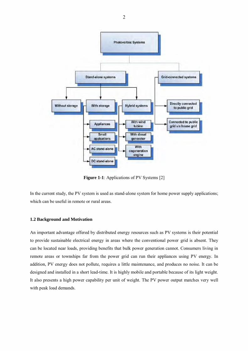
Photovoltaic energy sources can be used as stand-alone systems and grid-connected systems (see
Figure 1-1) and their applications include water pumping, battery charging, home power supplies,
street lighting, refrigeration, swimming-pool heating systems, hybrid vehicles, telecommunications,
military space and satellite power systems, and hydrogen production.
2
Figure 1-1: Applications of PV Systems [2]
In the current study, the PV system is used as stand-alone system for home power supply applications;
which can be useful in remote or rural areas.
1.2 Background and Motivation
An important advantage offered by distributed energy resources such as PV systems is their potential
to provide sustainable electrical energy in areas where the conventional power grid is absent. They
can be located near loads, providing benefits that bulk power generation cannot. Consumers living in
remote areas or townships far from the power grid can run their appliances using PV energy. In
addition, PV energy does not pollute, requires a little maintenance, and produces no noise. It can be
designed and installed in a short lead-time. It is highly mobile and portable because of its light weight.
It also presents a high power capability per unit of weight. The PV power output matches very well
with peak load demands.

3
The drawbacks of PV energy are as follows:
A high initial cost and low power conversion efficiency up to about 17% [2].
The non-linear current-voltage (I-V) characteristic exhibited by a PV cell due variations in
cell temperature and solar irradiation.
In a direct-coupled PV-load system, the power transferred from the PV generator source to
the load is rarely optimal and this has a negative effect on system efficiency.
Maximum power point trackers are used to extract the correct amount of current to run the system at
maximum power point (MPP). A complete solar panel equipped with an MPPT system includes a
solar panel, an MPPT algorithm, and a DC-DC converter topology. Several MPPT algorithms have
been proposed in the literature to track the maximum power of a PV system. These include the
Perturb and Observe (PO) method, the Incremental Conductance (IC) method, the Constant Voltage
(CV) method, and the fuzzy logic (FL) technique. These MPPT algorithms can be loaded onto either
in a personal computer or a microcontroller to perform maximum power tracking functions. However,
they differ in terms of speed, range of effectiveness, cost, the number of sensors required, complexity
and popularity [3]. The literature notes that existing classical algorithms used in the MPPT techniques
can be:
Fast to respond due to transient changes; or
Accurately to track, but not simultaneously.
Achieving both characteristics, rapid response and accurate tracking, features at the same time is the
ideal, because they can contribute greatly to reducing power losses caused by the dynamic tracking
errors that occur when environmental conditions change rapidly and increase overall efficiency.
The research questions of this dissertation are as follows:
Can an existing conventional MPPT algorithm be optimized in a residential PV system
application?
In what ways are the issues like the speed of response during the transient tracking operation
and power fluctuations at steady-state addressed under variable operating conditions?
1.3 Stand-alone Photovoltaic Simulation System Used
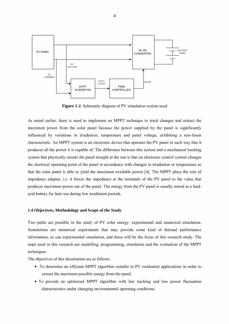
A general configuration of the current PV system comprises (Figure 1-2):
A stand-alone PV panel
An MPPT composed of a DC-DC converter topology along with its MPPT algorithm. An
inverter can be used when AC load is needed.
A battery bank as a storage device with its associated charger controllers.
4
Figure 1-2: Schematic diagram of PV simulation system used
As noted earlier, there is need to implement an MPPT technique to track changes and extract the
maximum power from the solar panel because the power supplied by the panel is significantly
influenced by variations in irradiation, temperature and panel voltage, exhibiting a non-linear
characteristic. An MPPT system is an electronic device that operates the PV panel in such way that it
produces all the power it is capable of. The difference between this system and a mechanical tracking
system that physically orients the panel straight at the sun is that an electronic control system changes
the electrical operating point of the panel in accordance with changes in irradiation or temperature so
that the solar panel is able to yield the maximum available power [4]. The MPPT plays the role of
impedance adapter, i.e. it forces the impedance at the terminals of the PV panel to the value that
produces maximum power out of the panel. The energy from the PV panel is usually stored in a lead-
acid battery for later use during low irradiation periods.
1.4 Objectives, Methodology and Scope of the Study
Two paths are possible in the study of PV solar energy: experimental and numerical simulation.
Simulations are numerical experiments that may provide some kind of thermal performance
information, as can experimental simulation, and these will be the focus of this research study. The
steps used in this research are modelling, programming, simulation and the evaluation of the MPPT
techniques.
The objectives of this dissertation are as follows:
To determine an efficient MPPT algorithm suitable in PV residential applications in order to
extract the maximum possible energy from the panel.
To provide an optimized MPPT algorithm with fast tracking and low power fluctuation
characteristics under changing environmental operating conditions.

5
The methodology adopted is as follows:
To investigate and understand the strengths and weaknesses of some classical MPPT algorithms
under variable operating conditions through a literature review.
To develop a PV model and MPPT model using Matlab and Simulink to assess the
performances of the existing MPPT algorithms and address their drawbacks by the use of
some optimization solutions suitable in PV residential applications.
A commercially available PV panel is modelled. Five MPPT algorithms are used in this dissertation
for the purposes of comparison. They are firstly written in Matlab m-files and investigated via
simulations. The standard Perturb and Observe (PO) algorithm, along with its two improved versions
and the conventional Incremental Conductance (IC) algorithm, also with its improved two-stage
version are assessed under sunny and cloudy weather operating conditions. Arising from this
comparison, the most efficient MPPT algorithm among the five is selected and implemented in the
whole PV system.
Finally, the performances of the most efficient algorithm when implemented in the complete PV
system and combined with the battery load is assessed and compared with its standard existing
version algorithm in a Matlab/Simulink environment to demonstrate its effectiveness under varying
weather conditions. The steady state and dynamic tracking performances of both implemented
algorithms are analyzed with regard to slow and rapid irradiance changes.
A complete PV system with an MPPT system including a solar panel, an MPPT algorithm, and a DC-
DC converter topology is mathematically modeled and simulated in a Matlab/Simulink environment
separately. After all subsystems have been verified one by one to ensure good functionality and
efficiency, they are connected together and combined with the battery load to assess the overall
performance of this residential PV application.
The aim of this project is not to design a controller loop for the PV voltage regulation or to perform a
cost analysis study of the MPPT techniques; rather it focuses on modelling, programming, simulation,
and evaluation of MPPT technique performances for a stand-alone PV system. There was no need to
build a prototype and assess it experimentally.
6
1.5 Outline of the thesis
The dissertation’s seven chapters are organized as follows:
Chapter one outlines the background and the motivation for the study and provides a schematic
diagram of the MPPT system used. The objectives, methodology and scope of the study are
highlighted.
Chapter two analyzes classical MPPT techniques (CV, PO, and IC methods) in the current literature
and addresses the issues of power fluctuations around MPP and lateness in tracking MPP by
investigating possible improvements under different weather conditions. Following the literature
review, an efficient MPPT algorithm is selected for further investigation in a Matlab programming
environment.
Chapter three deals with modelling and simulation of the PV panel via Matlab m-files and Simulink
blocks. Simple, two-diode, and one-diode PV cell models are explained. A one-diode Matlab and
Simulink model based on PV characteristic equations and manufacturer data is investigated. Finally,
the chapter presents a discussion on the simulated results.
In chapter four, five MPPT algorithms are written in Matlab m-files and investigated via simulations.
The Perturb and Observe (PO) algorithm along with its two improved versions and the conventional
Incremental Conductance (IC) algorithm, also with its two-stage improved version are assessed under
different environmental change conditions (sunny and cloudy weather). A discussion and comparison
of the simulated MPPT results follows.
A DC-DC converter topology and interface study based on the state space averaged model is
performed in chapter five to understand the steady state and dynamic behaviour of the buck and boost
converters. This helps to select the appropriate converter for the current PV system. The chosen
chopper is then modelled using a Simulink Power Systems toolbox.
Chapter six combine all the subsystems of PV system studied previously and analyzes the overall
performances of the PV system using the improved two-stage MPPT algorithm versus the classical
version under fast and slow irradiation changes.
Finally, in chapter seven, conclusions are presented concerning the simulated results of the study to
demonstrate the reasons for the choice of the MPPT algorithm used in the complete PV system. This
chapter also puts forward suggestions for future research on MPPT techniques in PV systems.
7
Chapter 2: LITERATURE SURVEY
2.1 Introduction
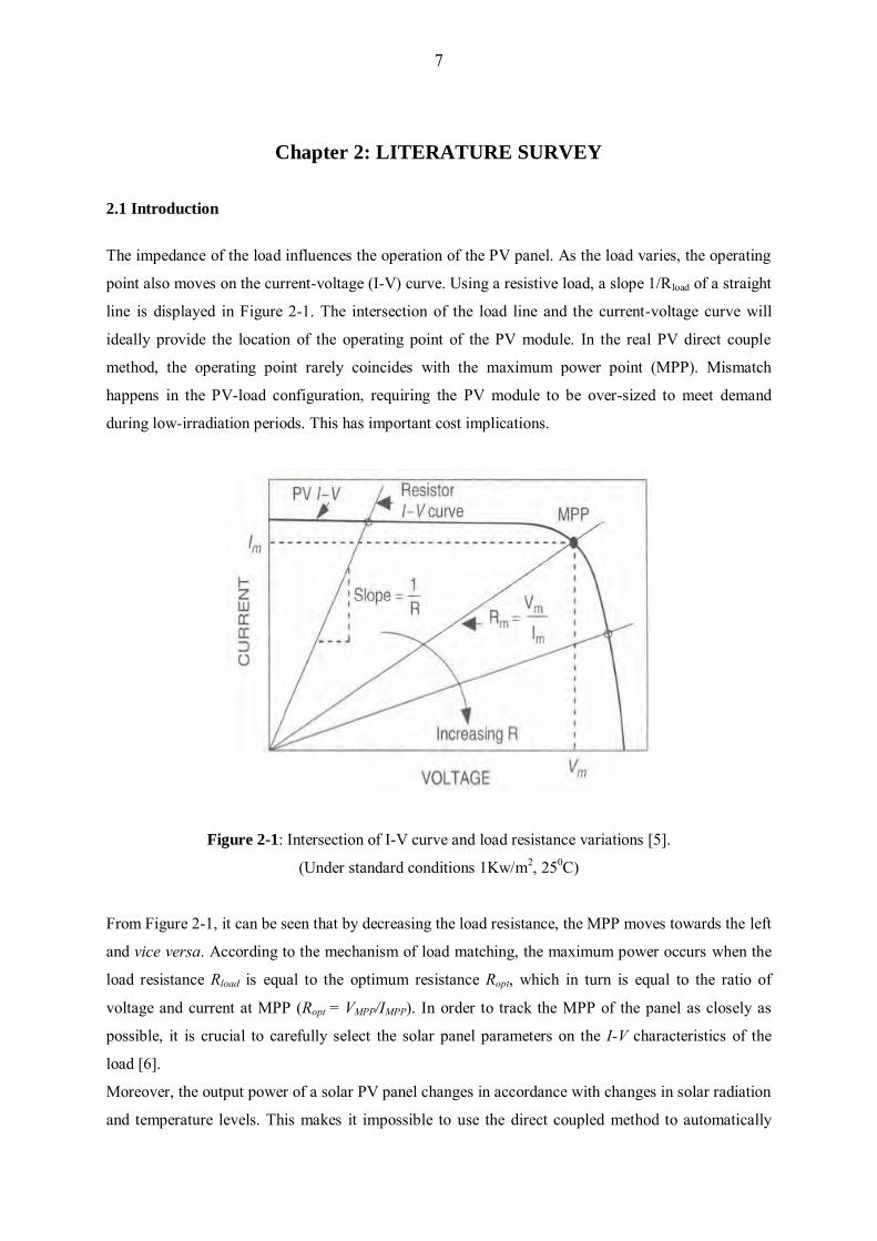
The impedance of the load influences the operation of the PV panel. As the load varies, the operating
point also moves on the current-voltage (I-V) curve. Using a resistive load, a slope 1/Rload of a straight
line is displayed in Figure 2-1. The intersection of the load line and the current-voltage curve will
ideally provide the location of the operating point of the PV module. In the real PV direct couple
method, the operating point rarely coincides with the maximum power point (MPP). Mismatch
happens in the PV-load configuration, requiring the PV module to be over-sized to meet demand
during low-irradiation periods. This has important cost implications.
Figure 2-1: Intersection of I-V curve and load resistance variations [5].
(Under standard conditions 1Kw/m2, 250C)
From Figure 2-1, it can be seen that by decreasing the load resistance, the MPP moves towards the left
and vice versa. According to the mechanism of load matching, the maximum power occurs when the
load resistance Rload is equal to the optimum resistance Ropt, which in turn is equal to the ratio of
voltage and current at MPP (Ropt = VMPP/IMPP). In order to track the MPP of the panel as closely as
possible, it is crucial to carefully select the solar panel parameters on the I-V characteristics of the
load [6].
Moreover, the output power of a solar PV panel changes in accordance with changes in solar radiation
and temperature levels. This makes it impossible to use the direct coupled method to automatically
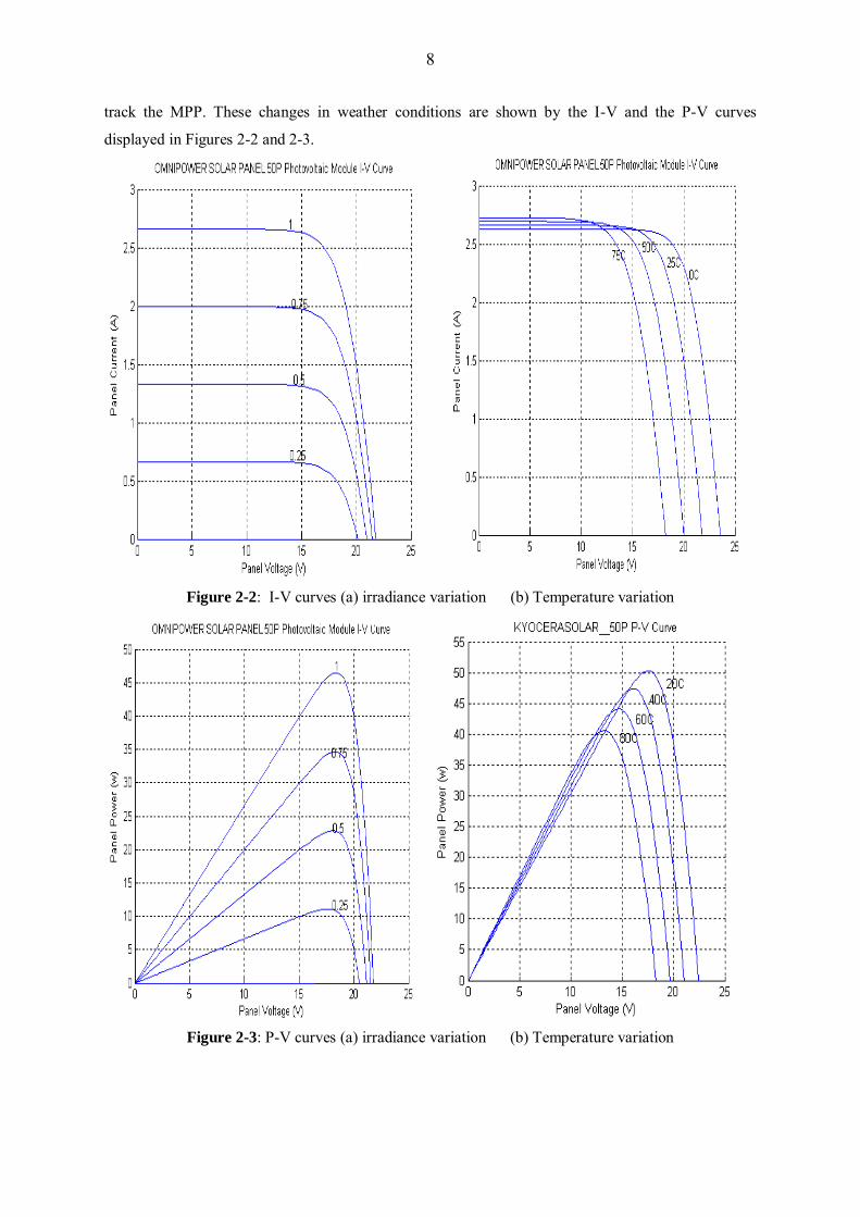
8
track the MPP. These changes in weather conditions are shown by the I-V and the P-V curves
displayed in Figures 2-2 and 2-3.
Figure 2-2: I-V curves (a) irradiance variation (b) Temperature variation
Figure 2-3: P-V curves (a) irradiance variation (b) Temperature variation
9
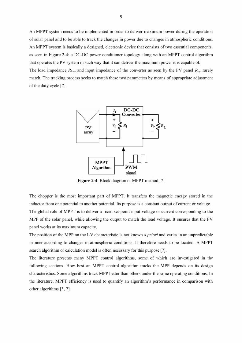
An MPPT system needs to be implemented in order to deliver maximum power during the operation
of solar panel and to be able to track the changes in power due to changes in atmospheric conditions.
An MPPT system is basically a designed, electronic device that consists of two essential components,
as seen in Figure 2-4: a DC-DC power conditioner topology along with an MPPT control algorithm
that operates the PV system in such way that it can deliver the maximum power it is capable of.
The load impedance Rload and input impedance of the converter as seen by the PV panel Ropt rarely
match. The tracking process seeks to match these two parameters by means of appropriate adjustment
of the duty cycle [7].
Figure 2-4: Block diagram of MPPT method [7]
The chopper is the most important part of MPPT. It transfers the magnetic energy stored in the
inductor from one potential to another potential. Its purpose is a constant output of current or voltage.
The global role of MPPT is to deliver a fixed set-point input voltage or current corresponding to the
MPP of the solar panel, while allowing the output to match the load voltage. It ensures that the PV
panel works at its maximum capacity.
The position of the MPP on the I-V characteristic is not known a priori and varies in an unpredictable
manner according to changes in atmospheric conditions. It therefore needs to be located. A MPPT
search algorithm or calculation model is often necessary for this purpose [7].
The literature presents many MPPT control algorithms, some of which are investigated in the
following sections. How best an MPPT control algorithm tracks the MPP depends on its design
characteristics. Some algorithms track MPP better than others under the same operating conditions. In
the literature, MPPT efficiency is used to quantify an algorithm’s performance in comparison with
other algorithms [3, 7].
10
2.2 Performance criteria of MPPT control algorithms
The following criteria are important in the design of the MPPT control algorithms:
2.2.1 Dynamic Response
A well-designed MPPT control algorithm needs to respond fast to sudden changes in atmospheric
conditions (solar irradiation and temperature) because the faster the tracking, the lower the loss of
solar energy.
2.2.2 Steady- state error
In steady-state analysis, it is essential to keep the system operating at MPP for as long as possible as
soon as MPP has been located. This level of accuracy is difficult to accomplish due to the active
perturbation process in conventional MPPT algorithms changes in weather conditions. A larger power
fluctuation may negatively affect the efficiency of the PV system.
2.2.3 Tracking Efficiency
Tracking efficiency is usually defined as the ratio of the electrical energy given as real power to
theoretical power during the same time period. The fewer the power losses observed, the higher the
output and efficiency of power. Some MPPT algorithms may perform better than others under the
same operating conditions. Therefore, a MPPT algorithm performance and comparison parameter,
often called tracking efficiency, is needed in order to quantify the performance of a specific MPPT
control algorithm under different operating conditions and to be able compare it with other MPPT
algorithms. In simulated PV systems, the tracking efficiency can be estimated as follows [8, 9, and
10]:
n
i ith
irealMPPT P
Pn max,
,1 (2.1)
In the above equation Preal represents the real power received by the load and Pthmax is the theoretical
maximum power available at the PV module with n, the number of samples.
2.3 MPPT control algorithms classification
Algorithms already exist to track the maximum power for a PV system. In the seeking algorithms,
there are some indirect control or “quasi seeking methods” such as the look-up table method, the
constant voltage (CV) method, the short-circuit current (SC) method, and the direct control or “true
seeking methods”. True seeking methods include the Perturb & Observe (PO) method, the
incremental conductance (IC) method, and finally artificial intelligence methods such as fuzzy logic
control (FLC) MPPT technique, and the neural network method. The indirect control methods can be
characterized by the fact that the MPP is estimated either from measurements of the voltage and
11
current of the solar panel, the irradiance, or by the use of empirical data through numerical
approximations. These methods are therefore not appropriate when changes occur in irradiance or
temperature [10]. In contrast, the true seeking methods are able to obtain actual maximum power
when variations occur in weather conditions. One or two variables may be used in the seeking
process. PO and IC are two-variable methods because they require the measurement of two variables
to calculate the maximum power, and PV output voltage and current while SC and CV methods use
only one variable to control either PV output current or voltage respectively.
2.4 Simple Panel-load matching
This system represents simple PV battery chargers. In this method of operating the PV panel close to
MPP, the operating point is obtained under average operating conditions by a series of measurements.
Once the values for maximum power current and voltage respectively IMPP, VMPP are found, a
matching load can be designed. The whole system is devised in such a way that the average battery
voltage is near to the average VMPP. The advantage of this configuration resides in its simplicity, i.e. it
requires no extra circuitry but it does not take into account any changes in insolation or temperature
levels. Maximum power point tracking is therefore not possible because it doesn’t take into
consideration changes in VMPP.
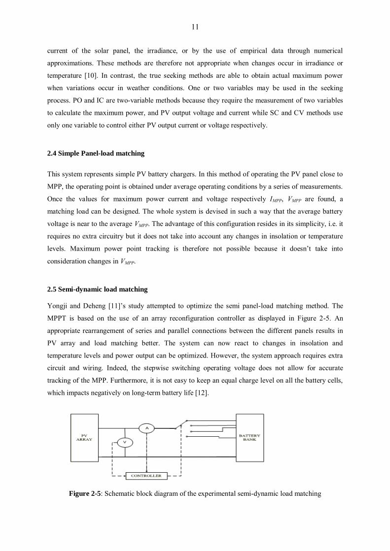
2.5 Semi-dynamic load matching Yongji and Deheng [11]’s study attempted to optimize the semi panel-load matching method. The
MPPT is based on the use of an array reconfiguration controller as displayed in Figure 2-5. An
appropriate rearrangement of series and parallel connections between the different panels results in
PV array and load matching better. The system can now react to changes in insolation and
temperature levels and power output can be optimized. However, the system approach requires extra
circuit and wiring. Indeed, the stepwise switching operating voltage does not allow for accurate
tracking of the MPP. Furthermore, it is not easy to keep an equal charge level on all the battery cells,
which impacts negatively on long-term battery life [12].
Figure 2-5: Schematic block diagram of the experimental semi-dynamic load matching
12
2.6 Voltage feedback methods
This system doesn’t need battery. Instead, a simple MPPT method is used to keep the array or panel
voltage close to the MPP by adjusting and trying to match the array voltage to the reference voltage
VMPP.
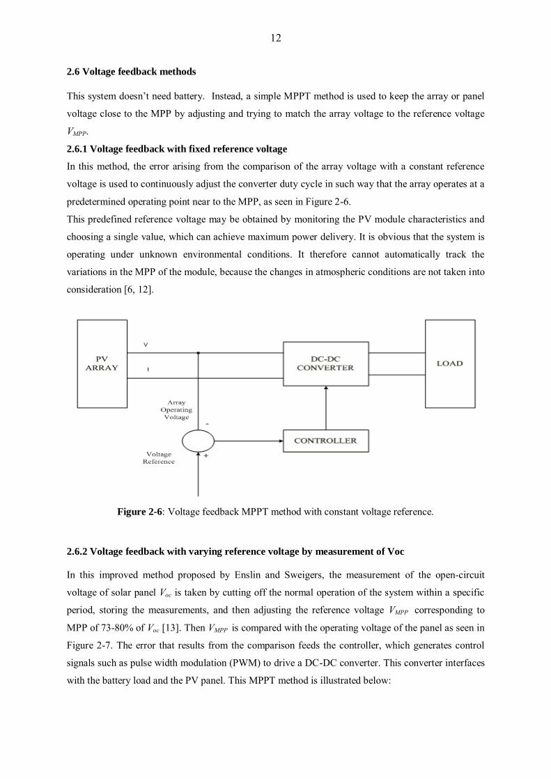
2.6.1 Voltage feedback with fixed reference voltage
In this method, the error arising from the comparison of the array voltage with a constant reference
voltage is used to continuously adjust the converter duty cycle in such way that the array operates at a
predetermined operating point near to the MPP, as seen in Figure 2-6.
This predefined reference voltage may be obtained by monitoring the PV module characteristics and
choosing a single value, which can achieve maximum power delivery. It is obvious that the system is
operating under unknown environmental conditions. It therefore cannot automatically track the
variations in the MPP of the module, because the changes in atmospheric conditions are not taken into
consideration [6, 12].
Figure 2-6: Voltage feedback MPPT method with constant voltage reference.
2.6.2 Voltage feedback with varying reference voltage by measurement of Voc
In this improved method proposed by Enslin and Sweigers, the measurement of the open-circuit
voltage of solar panel Voc is taken by cutting off the normal operation of the system within a specific
period, storing the measurements, and then adjusting the reference voltage VMPP corresponding to
MPP of 73-80% of Voc [13]. Then VMPP is compared with the operating voltage of the panel as seen in
Figure 2-7. The error that results from the comparison feeds the controller, which generates control
signals such as pulse width modulation (PWM) to drive a DC-DC converter. This converter interfaces
with the battery load and the PV panel. This MPPT method is illustrated below:
13
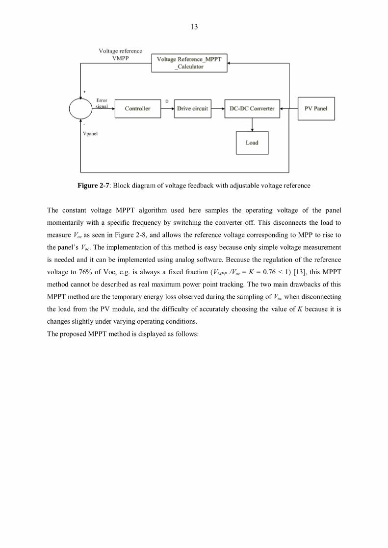
Figure 2-7: Block diagram of voltage feedback with adjustable voltage reference
The constant voltage MPPT algorithm used here samples the operating voltage of the panel
momentarily with a specific frequency by switching the converter off. This disconnects the load to
measure Voc as seen in Figure 2-8, and allows the reference voltage corresponding to MPP to rise to
the panel’s Voc. The implementation of this method is easy because only simple voltage measurement
is needed and it can be implemented using analog software. Because the regulation of the reference
voltage to 76% of Voc, e.g. is always a fixed fraction (VMPP /Voc = K = 0.76 < 1) [13], this MPPT
method cannot be described as real maximum power point tracking. The two main drawbacks of this
MPPT method are the temporary energy loss observed during the sampling of Voc when disconnecting
the load from the PV module, and the difficulty of accurately choosing the value of K because it is
changes slightly under varying operating conditions.
The proposed MPPT method is displayed as follows:
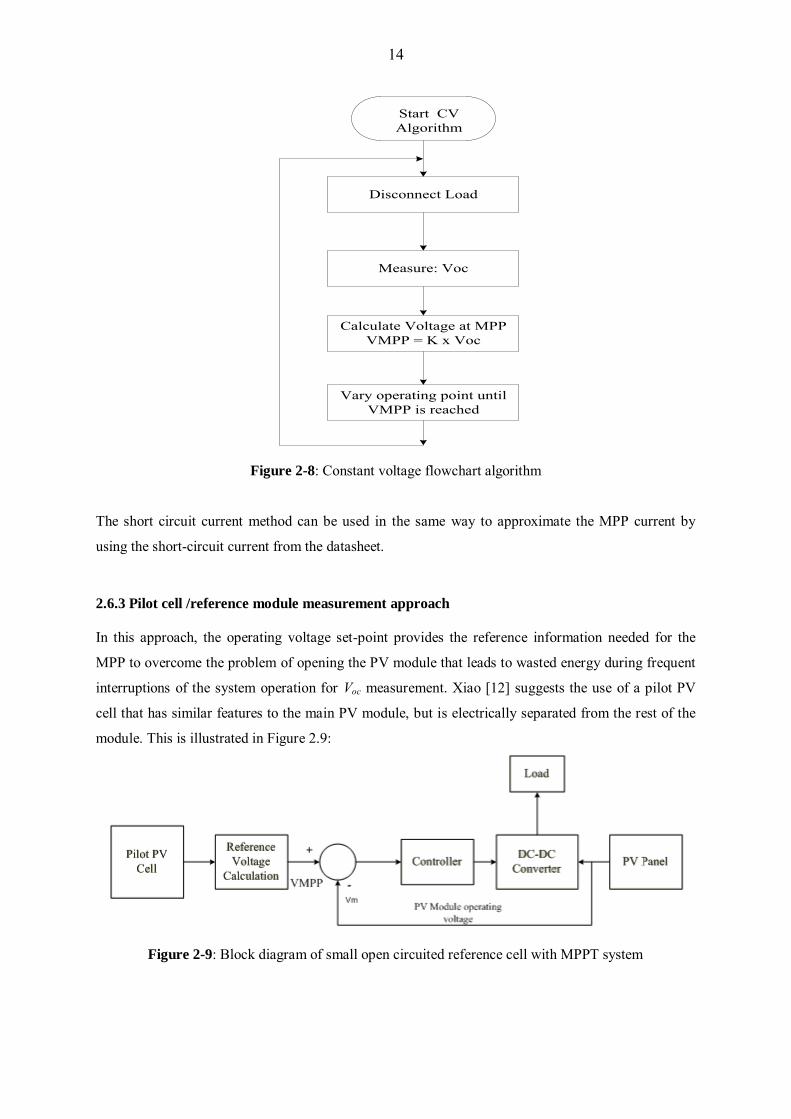
14
Vary operating point until VMPP is reached
Calculate Voltage at MPPVMPP = K x Voc
Measure: Voc
Start CV Algorithm
Disconnect Load
Figure 2-8: Constant voltage flowchart algorithm
The short circuit current method can be used in the same way to approximate the MPP current by
using the short-circuit current from the datasheet.
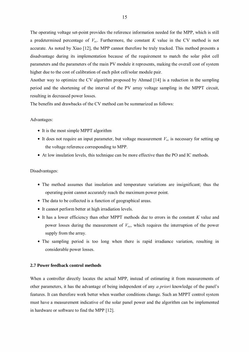
2.6.3 Pilot cell /reference module measurement approach
In this approach, the operating voltage set-point provides the reference information needed for the
MPP to overcome the problem of opening the PV module that leads to wasted energy during frequent
interruptions of the system operation for Voc measurement. Xiao [12] suggests the use of a pilot PV
cell that has similar features to the main PV module, but is electrically separated from the rest of the
module. This is illustrated in Figure 2.9:
Figure 2-9: Block diagram of small open circuited reference cell with MPPT system
15
The operating voltage set-point provides the reference information needed for the MPP, which is still
a predetermined percentage of Voc. Furthermore, the constant K value in the CV method is not
accurate. As noted by Xiao [12], the MPP cannot therefore be truly tracked. This method presents a
disadvantage during its implementation because of the requirement to match the solar pilot cell
parameters and the parameters of the main PV module it represents, making the overall cost of system
higher due to the cost of calibration of each pilot cell/solar module pair.
Another way to optimize the CV algorithm proposed by Ahmad [14] is a reduction in the sampling
period and the shortening of the interval of the PV array voltage sampling in the MPPT circuit,
resulting in decreased power losses.
The benefits and drawbacks of the CV method can be summarized as follows:
Advantages:
It is the most simple MPPT algorithm
It does not require an input parameter, but voltage measurement Voc is necessary for setting up
the voltage reference corresponding to MPP.
At low insulation levels, this technique can be more effective than the PO and IC methods.
Disadvantages:
The method assumes that insolation and temperature variations are insignificant; thus the
operating point cannot accurately reach the maximum power point.
The data to be collected is a function of geographical areas.
It cannot perform better at high irradiation levels.
It has a lower efficiency than other MPPT methods due to errors in the constant K value and
power losses during the measurement of Voc, which requires the interruption of the power
supply from the array.
The sampling period is too long when there is rapid irradiance variation, resulting in
considerable power losses.
2.7 Power feedback control methods
When a controller directly locates the actual MPP, instead of estimating it from measurements of
other parameters, it has the advantage of being independent of any a priori knowledge of the panel’s
features. It can therefore work better when weather conditions change. Such an MPPT control system
must have a measurement indicative of the solar panel power and the algorithm can be implemented
in hardware or software to find the MPP [12].
16
2.7.1 Perturb and Observe Control Algorithm
The Perturb and observe (PO) algorithm is one of the most used algorithms due to its simplicity and
easy implementation. This MPPT method is also known as the Hill Climbing (HC) algorithm.
The difference between PO and HC may be explained by the fact that the HC requires a change in the
converter duty cycle, while the PO perturbs the operating voltage of the PV panel; but the working
principle is the same for both [15].
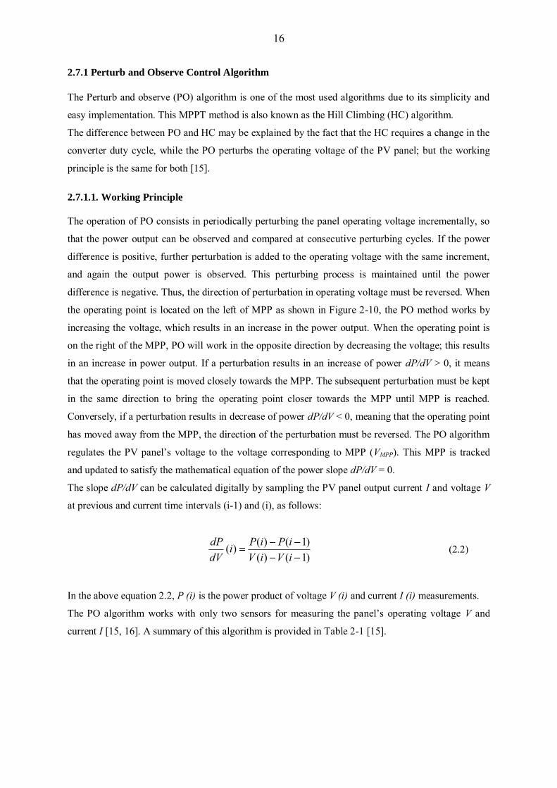
2.7.1.1. Working Principle
The operation of PO consists in periodically perturbing the panel operating voltage incrementally, so
that the power output can be observed and compared at consecutive perturbing cycles. If the power
difference is positive, further perturbation is added to the operating voltage with the same increment,
and again the output power is observed. This perturbing process is maintained until the power
difference is negative. Thus, the direction of perturbation in operating voltage must be reversed. When
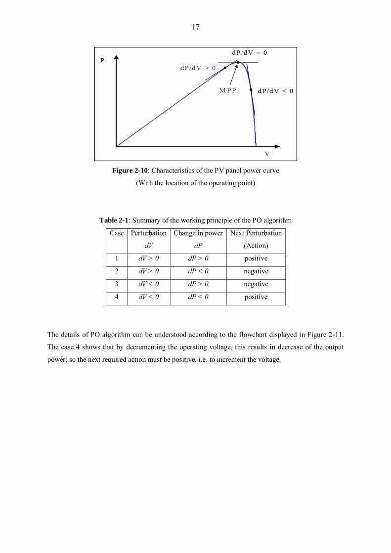
the operating point is located on the left of MPP as shown in Figure 2-10, the PO method works by
increasing the voltage, which results in an increase in the power output. When the operating point is
on the right of the MPP, PO will work in the opposite direction by decreasing the voltage; this results
in an increase in power output. If a perturbation results in an increase of power dP/dV > 0, it means
that the operating point is moved closely towards the MPP. The subsequent perturbation must be kept
in the same direction to bring the operating point closer towards the MPP until MPP is reached.
Conversely, if a perturbation results in decrease of power dP/dV < 0, meaning that the operating point
has moved away from the MPP, the direction of the perturbation must be reversed. The PO algorithm
regulates the PV panel’s voltage to the voltage corresponding to MPP (VMPP). This MPP is tracked
and updated to satisfy the mathematical equation of the power slope dP/dV = 0.
The slope dP/dV can be calculated digitally by sampling the PV panel output current I and voltage V
at previous and current time intervals (i-1) and (i), as follows:
)1()()1()()(
iViViPiPi
dVdP
(2.2)
In the above equation 2.2, P (i) is the power product of voltage V (i) and current I (i) measurements.
The PO algorithm works with only two sensors for measuring the panel’s operating voltage V and
current I [15, 16]. A summary of this algorithm is provided in Table 2-1 [15].
17
Figure 2-10: Characteristics of the PV panel power curve
(With the location of the operating point)
Table 2-1: Summary of the working principle of the PO algorithm
Case Perturbation
dV
Change in power
dP
Next Perturbation
(Action)
1 dV > 0 dP > 0 positive
2 dV > 0 dP < 0 negative
3 dV < 0 dP > 0 negative
4 dV < 0 dP < 0 positive
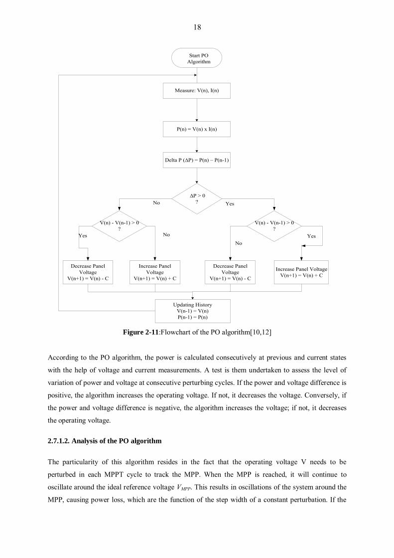
The details of PO algorithm can be understood according to the flowchart displayed in Figure 2-11.
The case 4 shows that by decrementing the operating voltage, this results in decrease of the output
power; so the next required action must be positive, i.e. to increment the voltage.
18
∆P > 0?
V(n) - V(n-1) > 0 ?
V(n) - V(n-1) > 0?
Decrease Panel Voltage
V(n+1) = V(n) - C
Increase Panel Voltage
V(n+1) = V(n) + C
Decrease Panel Voltage
V(n+1) = V(n) - C
Increase Panel VoltageV(n+1) = V(n) + C
Updating HistoryV(n-1) = V(n)P(n-1) = P(n)
Delta P (∆P) = P(n) – P(n-1)
P(n) = V(n) x I(n)
Measure: V(n), I(n)
No
Start PO Algorithm
No YesYes
No Yes
Figure 2-11:Flowchart of the PO algorithm[10,12]
According to the PO algorithm, the power is calculated consecutively at previous and current states
with the help of voltage and current measurements. A test is them undertaken to assess the level of
variation of power and voltage at consecutive perturbing cycles. If the power and voltage difference is
positive, the algorithm increases the operating voltage. If not, it decreases the voltage. Conversely, if
the power and voltage difference is negative, the algorithm increases the voltage; if not, it decreases
the operating voltage.
2.7.1.2. Analysis of the PO algorithm
The particularity of this algorithm resides in the fact that the operating voltage V needs to be
perturbed in each MPPT cycle to track the MPP. When the MPP is reached, it will continue to
oscillate around the ideal reference voltage VMPP. This results in oscillations of the system around the
MPP, causing power loss, which are the function of the step width of a constant perturbation. If the

19
fixed step increment selected is large, the PO algorithm will speed up its response under transient
operating conditions with the trade-off of increased fluctuations. By diminishing the perturbation step
size, the oscillations can be reduced; thus the power losses are minimized. Nevertheless, this causes
the system to slow down its response when subjected to rapid changes in weather conditions,
compromising its dynamic performances.
It should be noted that a small constant step perturbation size hampered dynamic performance, while
a large one leads to poor steady-state performance. There is always a trade-off between high accuracy
(low power fluctuation) at steady state and a fast response due to dynamic changes in atmospheric
conditions. The value of the suitable step width of the perturbation is a function of the system used
and it is usually tuned experimentally, as discussed by Xiao [12].
Moreover, the PO control algorithm may go in the wrong direction and fail to react properly when
subjected to sudden changes in environmental parameters. In this specific condition, the PO algorithm
is unable to precisely interpret the increase in power, either due to the previous perturbation of the
voltage or to an increase in insolation. It, then fails to react in order to avoid the operating point going
away from the MPP as explained by Hohm [8].
The benefits of the PO method are as follows:
It is simple and easy to implement.
It is cheap, requiring only panel voltage and current measurements.
It is effective when the insolation changes slowly over time.
The drawbacks of PO method are as follows:
Although the MPP is reached, the operating point continues to oscillate around the MPP,
resulting in PV power losses.
The PO fails to work properly under a sudden increase in insolation level, exhibiting erratic
behaviour.
It lacks accuracy in finding whether the MPP is reached.
A small constant step perturbation size leads to high accuracy but hampers dynamic
performance.
A large constant step perturbation size leads to fast tracking, but the accuracy of the tracking
suffers (poor steady-state performance).
20
2.7.2 Incremental Conductance Control Algorithm
The Incremental Conductance (IC) method was proposed in order to overcome the drawbacks
of the PO algorithm when subjected to fast changing environmental conditions. With the help
of voltage and current measurements, the conductance I/V and incremental conductance dI/dV
are determined so that the decision can be made to increase or decrease the operating voltage
according to the operating point on the left or the right of the MPP respectively.
2.7.2.1 Working Principle
The working principle of the IC method relies on the fact that the slope of the PV panel power curve
is negative on the right of the MPP, zero at the MPP and positive on the left of the MPP as follows:
dP/dV > 0 left of MPP (V< VMPP)
dP/dV = 0 at MPP (V=VMPP) (2.3)
dP/dV < 0 right of MPP (V >VMPP)
Knowing that P = VI, the slope of power curve at MPP can be written as:
0
dVdIVI
dVdIV
dVdVI
dVdP
(2.4)
(2.3) may be written as:
dI/dV < -I/V right of MPP
dI/dV = -I/V at MPP (2.5)
dI/dV > -I/V left of MPP
According to equation 2.5, the incremental conductance (IC) algorithm provides enough information
to locate the MPP. This is made possible by means of the respective measurement and comparison of,
dI/dV and I/V. VMPP is the set-point reference voltage corresponding to the MPP at which the PV
module is required to operate. The detailed working principle of the IC algorithm can be understood
by means of the following flow chart.
21
∆V = 0?
∆I > 0 ?
dI/dV > -I/V?
Decrease Panel Voltage
V(n+1) = V(n) - C
Increase Panel Voltage
V(n+1) = V(n) + C
Decrease Panel Voltage
V(n+1) = V(n) - C
Increase Panel VoltageV(n+1) = V(n) + C
Updating HistoryV(n-1) = V(n)I(n-1) = I(n)
∆I (n) = I(n) – I(n-1)
∆V(n) = V(n) - V(n-1)
Measure: V(n), I(n)
No
Start IC Algorithm
Yes YesNo
dI/dV= -I/V ∆I=0
YesNo
Yes Yes
NoNo
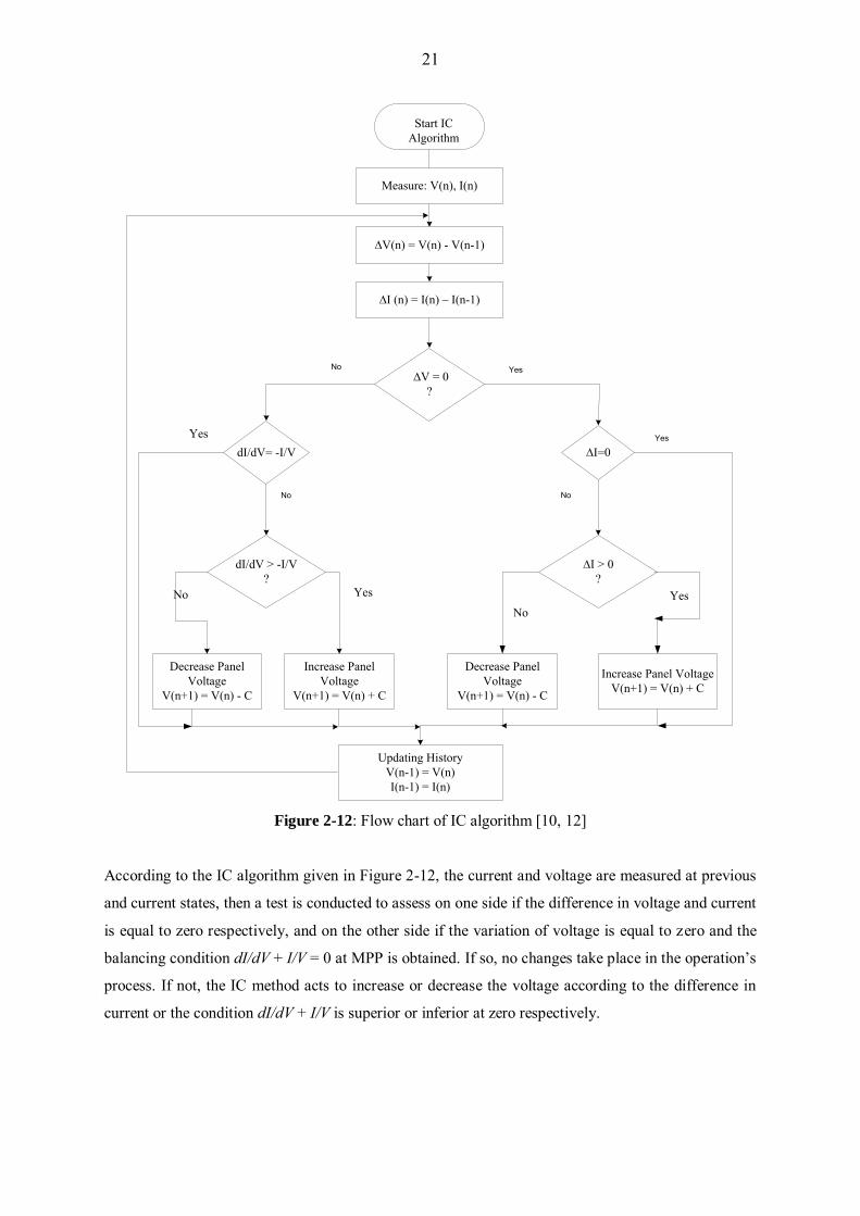
Figure 2-12: Flow chart of IC algorithm [10, 12]
According to the IC algorithm given in Figure 2-12, the current and voltage are measured at previous
and current states, then a test is conducted to assess on one side if the difference in voltage and current
is equal to zero respectively, and on the other side if the variation of voltage is equal to zero and the
balancing condition dI/dV + I/V = 0 at MPP is obtained. If so, no changes take place in the operation’s
process. If not, the IC method acts to increase or decrease the voltage according to the difference in
current or the condition dI/dV + I/V is superior or inferior at zero respectively.

22
2.7.2.2. Analysis of the IC algorithm
The IC algorithm performs much better than PO when rapidly changing weather conditions occur [6,
12]. Its advantages reside in the fact that it doesn’t oscillate around the MPP. According to the above
flowchart, at the MPP, the condition dI/dV = -I/V is true and no change occurs in operating voltage
because the operating voltage is equal to the voltage at MPP. The aforementioned condition and the
difference in current dI = 0 allows it to bypass the adjustment perturbation step and the current cycle
ends. According to the working principle, the conditions 0VI
dVdI
and dI > 0 allow the relative
location of the MPP. This provides the guarantee that an initial adjustment in the wrong direction, as
observed with the “trial and error” PO algorithm, does not happen. A quick and correct system
response to fast increasing insolation levels conditions should be expected, resulting in high system
efficiency when compared to the PO method. If the difference in current dI = 0 is not achieved
according to the flowchart in Figure 2-12, the test condition dI > 0 is used to establish if the system is
operating at the left or right of the MPP and a subsequent adjustment of the operating voltage needs to
be made.
The experiments revealed that some oscillations are still present under stable atmospheric conditions
because the condition dP/dV = 0 or dI/dV = -I/V only rarely occurred in practical terms. This may be
caused by the approximations made for dV, dI and the difficulty in regulating V to the exact VMPP
when using a constant perturbation step size. There is still a trade-off between fast tracking and high
accuracy, which rely on the step size of the single perturbation. A possible solution to effectively
perform the IC algorithm, can be achieved by the use of dI/dV and I/V to generate an error signal
err = I/V + dI/dV [15]. The value of the error is optimized by considering the risk of oscillation of the
operating point around the MPP and the amount of steady-state tracking error at the same point of the
MPP.
The benefits of the IC method can be summarised as follows:
It is more effective at high solar irradiation levels than the PO algorithm.
Theoretically, the MPP can be located and reached; therefore, the perturbation can be
bypassed and stopped.
It only requires panel voltage and current measuring sensors, because the incremental changes
can be approximated by comparing current and previous measurements.
23
The drawbacks of the IC method are as follows:
It is more complex to implement compared with the PO.
It requires compulsory measurement of PV voltage and current.
When the fixed step increment is decreased to improve the accuracy of tracking, dynamic
performance suffers because the system slows. This results in a trade-off.
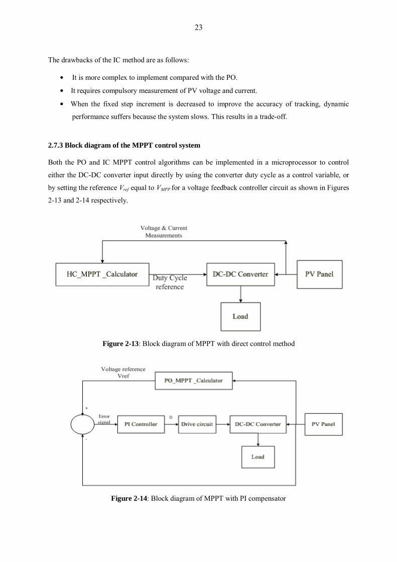
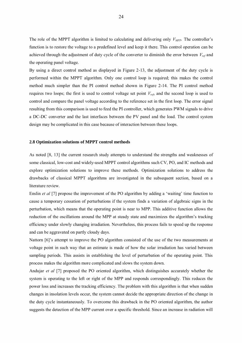
2.7.3 Block diagram of the MPPT control system
Both the PO and IC MPPT control algorithms can be implemented in a microprocessor to control
either the DC-DC converter input directly by using the converter duty cycle as a control variable, or
by setting the reference Vref equal to VMPP for a voltage feedback controller circuit as shown in Figures
2-13 and 2-14 respectively.
Figure 2-13: Block diagram of MPPT with direct control method
Figure 2-14: Block diagram of MPPT with PI compensator
24
The role of the MPPT algorithm is limited to calculating and delivering only VMPP. The controller’s
function is to restore the voltage to a predefined level and keep it there. This control operation can be
achieved through the adjustment of duty cycle of the converter to diminish the error between Vref and
the operating panel voltage.
By using a direct control method as displayed in Figure 2-13, the adjustment of the duty cycle is
performed within the MPPT algorithm. Only one control loop is required; this makes the control
method much simpler than the PI control method shown in Figure 2-14. The PI control method
requires two loops; the first is used to control voltage set point Vref, and the second loop is used to
control and compare the panel voltage according to the reference set in the first loop. The error signal
resulting from this comparison is used to feed the PI controller, which generates PWM signals to drive
a DC-DC converter and the last interfaces between the PV panel and the load. The control system
design may be complicated in this case because of interaction between these loops.
2.8 Optimization solutions of MPPT control methods
As noted [8, 13] the current research study attempts to understand the strengths and weaknesses of
some classical, low-cost and widely-used MPPT control algorithms such CV, PO, and IC methods and
explore optimization solutions to improve these methods. Optimization solutions to address the
drawbacks of classical MPPT algorithms are investigated in the subsequent section, based on a
literature review.
Enslin et al [7] propose the improvement of the PO algorithm by adding a ‘waiting’ time function to
cause a temporary cessation of perturbations if the system finds a variation of algebraic signs in the
perturbation, which means that the operating point is near to MPP. This additive function allows the
reduction of the oscillations around the MPP at steady state and maximizes the algorithm’s tracking
efficiency under slowly changing irradiation. Nevertheless, this process fails to speed up the response
and can be aggravated on partly cloudy days.
Nattorn [6]’s attempt to improve the PO algorithm consisted of the use of the two measurements at
voltage point in such way that an estimate is made of how the solar irradiation has varied between
sampling periods. This assists in establishing the level of perturbation of the operating point. This
process makes the algorithm more complicated and slows the system down.
Andujar et al [7] proposed the PO oriented algorithm, which distinguishes accurately whether the
system is operating to the left or right of the MPP and responds correspondingly. This reduces the
power loss and increases the tracking efficiency. The problem with this algorithm is that when sudden
changes in insolation levels occur, the system cannot decide the appropriate direction of the change in
the duty cycle instantaneously. To overcome this drawback in the PO oriented algorithm, the author
suggests the detection of the MPP current over a specific threshold. Since an increase in radiation will
25
result in an increase in the value of the MPP current, the algorithm is required to detect the variation
of current over a certain threshold and respond correspondingly with an immediate increase in duty
cycle. The increase in duty cycle implies a reduction in the input impedance of the DC-DC converter
and obliges the PV panel to displace towards the higher current point close to the MPP.
When the change in irradiation intensity results in a significant change in power, rather than from the
operating voltage perturbation, the PO algorithm can get confused. It interprets the change in the
power as an effect of voltage perturbation. To solve this problem, Sera [16] proffers an improved PO
algorithm that proposes supplementary power measurement between two MPPT sampling periods. It
uses this information to distinguish the actions caused by the effects of the environment from the
perturbation of the MPPT. The experimental results show that the improved PO can avoid deviations
in the wrong direction due to fast changes in irradiation, improving the efficiency of the algorithm.
Jain and Agarwal [17] propose a new and fast algorithm for tracking the MPP in PV systems, in
which a variable step-size is used to rapidly approximate the MPP. The disadvantage caused by a
small, rather than variable step-size during the complete tracking operation is removed, resulting in a
diminished number of iterations and hence fast tracking in comparison to standard MPPT methods.
Two stages are required in the working process of the algorithm.
The operating point is quickly brought into the first mode within close range of the actual MPP using
an intermediate variable obtained by analysis rather than tracking power, facilitating fast tracking.
The second mode consists of a conventional scheme (PO or IC algorithm) to bring the operating point
even closer to the exact MPP, resulting in better accuracy because it tracks the power with fine steps.
The benefit of this algorithm lies in tracking an intermediate variable, which has a single-to-single
direct relationship with the duty cycle, rather than tracking power itself. However, the algorithm uses
a variable step-size iteration that needs to be carefully analyzed because it varies in magnitude due to
changes in temperature and insolation at MPP. The proposed algorithm yields better efficiencies
under a transient tracking mode in comparison with conventional methods and is more applicable in
rapidly changing atmospheric conditions.
Milosevic [18], proposed a modified version of the PO algorithm to counter oscillations around the
MPP without reducing the increment (or step size) of the algorithm. This modification lies in the fact
that the condition dP >0 is presently split into two parts with dP > e and –dP < e with the parameter
e, which is the approximated value of the range of the power oscillations. With the modified PO
algorithm, there are no oscillations in the duty ratio, leading to improved performance in terms of
power oscillations and fast response under slowly changing environmental conditions but it fails to
track the MPP correctly under when environmental conditions change suddenly.
Another modified PO algorithm presented by Xiao [12] includes an additional insolation control loop.
If there is a large and sudden change in the PV output current as a result of the abrupt change in
isolation, a current change threshold “e” needs to be defined as a system parameter. The direction of
the panel output current can be used to directly control the perturbation of the panel reference voltage.
26
Fast tracking is achieved by means of this additional insolation control loop, but the difficulties in
choosing the appropriate width step size to achieve better steady state features remain unsolved.
Moreover, the current change threshold e = I(k) – I(k-1) at successive steps is difficult to determine.
A modified adaptive high climbing method has been developed by Bircan and Xiao [5, 12], to
improve the high climbing algorithm through solving the problem of a fixed increment step of the
duty cycle “b”. It makes “b” large in order to speed up its response during the transient mode and “b”
small to accurately reduce the fluctuations at steady state with on-line tuning of the parameter.
“b” is linear equation given as follows: b(k) =)1(* kb
PM
With a constant variable M and P difference in power at consecutive period times.
The modified adaptive hill climbing method provides good performance in terms of both dynamic
response and steady-state stage when compared with the standard adaptive hill climbing (AHC)
method. The drawbacks of the AHC control algorithm in terms of giving wrong control signals under
sudden change of insolation were corrected.
An improved MPPT method for PV systems is proposed by Tafticht [19]. His new method is based on
experimental measurements of Voc of the PV module to locate the MPP, and this approach uses a non-
linear expression for the operating voltage based on Voc. The experimental results show better steady
state performance, which results in increased average efficiency of the MPPT. No tests were
performed to assess the dynamic performance of the system under slow and rapidly changing
environmental conditions.
Different PO (or high climbing) MPPT algorithms are tested by Yafaoui and Wu [20] under sudden
changes in atmospheric conditions. These include the PO, modified PO (MPO), and Estimate Perturb
and Perturb (EPP) algorithms. The PO modified version 1(or MPO) is assigned to correct the
limitations of the PO algorithm under sudden changes in weather conditions, leading to incorrect or
slow MPPT. It isolates the oscillations resulting from weather changes from those happened as a
result of increasing or decreasing the voltage. This is made possible by adding an irradiance-changing
estimate parameter to determine the rate of power change caused by a variation in weather conditions.
The PO modified version 2 (or EPP) was then introduced to improve the speed of the PO modified
version 1 algorithm while maintaining its high tracking accuracy.
This is made possible by the use of one estimate parameter for every two perturbation modes to
improve the tracking speed, while maintaining the tracking accuracy of the MPO algorithm. Thus, the
PO modified version 2 show obvious advantages over its version 1.
The experimental results show that the EPP algorithm yields the similar accuracy as the MPO
algorithm, but tracks 50% faster. When compared with the standard PO algorithm, it achieved the
same speed with much higher accuracy. Its overall performance is therefore superior to both the PO
and PO modified version 1 algorithms.
27
Shen [21] proposes a modified PO method to improve the shortcomings of the prior PO MPPT
algorithm. It provides a conveniently regulated capability of the perturbation, which stops the
perturbation while tracking to close the MPP.
The MPPT algorithm is executed in three stages that make the process longer and more complex, but
the modification improves the system’s dynamic response and the power consumption of the
traditional PO algorithm.
An improvement on the IC algorithm has been suggested by Wang and Xu [22], who attempted to
execute corresponding tracking approaches at different situations. This allows the proposed algorithm
to achieve both fast and fine tracking characteristics simultaneously.
Furthermore, the energy losses caused by dynamic tracking errors under sudden changes in
atmospheric conditions are reduced. At start-up and when the weather changes suddenly fast tracking
is needed mere than during normal operations. Fast and fine tracking approaches are executed
respectively by the constant voltage and the incremental conductance algorithms. The decision on the
appropriate tracking approach is made by monitoring the variation of the PV panel output current. The
particularity of this algorithm rests on the fact that the accurate tracking and the fast transient speed
response are separately devised, providing the possibility of setting the perturbation step to a very
small size. This results in higher tracking accuracy when compared with the conventional incremental
conductance IC algorithm where the width step size needs to be balanced to meet accuracy and
tracking speed requirements.
Lee and Cho [23] suggest an updated IC MPPT algorithm where step size varies. The change in a step
size relies upon the inherent characteristic of the solar panel. The particularity of this algorithm as
explained by Lee [24] lies in the fact that a constant resistance control method uses an internal loop
for the parallel stabilization and operation of solar panel system. The experimental implementation
test of the proposed MPPT method includes prototype solar panel system hardware consisting of a
parallel connected buck converter and a constant resistance control algorithm. This proposed approach
is implemented, built and tested and can adjust a step size automatically to a solar panel operating
point, thereby improving the accuracy and speed response in comparison with the conventional IC,
which uses a fixed step increment.
Another innovative way to track algorithm improvement is made by Yu [25], and consists of
improving the efficiency of the PV power generation system at different solar irradiance levels.
PO and IC algorithms are not effective under rapid changes at lower insolation, and fail to track the
MPP. Under these same conditions, the constant voltage control algorithm is more effective and much
better at tracking the MPP. Moreover, the IC algorithm offers better performance under rapid changes
at higher insolation when compared with the PO algorithm. These two strengths using the CV and IC
MPPT algorithms respectively have been combined to provide an efficient two-mode control
algorithm. The two-stage MPPT algorithm yields better performances not only at higher, but also at
lower, irradiation. The disadvantage of this MPPT algorithm lies in the fact that its practical
28
implementation requires precise measurement of radiation; this increases the overall costs of the PV
installation.
A DC-DC converter topology and interface study between the panel and the battery load was
performed by Xiao [26], who evaluated the response of buck and boost converters for the MPPT and
suggested the best option for their use in a PV system. The methodology based on the state space
averaged model to understand the steady state behavior based on design specifications and the
dynamic behavior using root locus and bode methods for the buck and boost choppers and then
selecting the appropriate converter. The steady-state and dynamic analysis show that the boost
converter outperformed the buck chopper because of cheaper components, better damping factors and
overshoot of unit step response and was selected to be implemented in their PV application.
Mahdi [27] proposes a PO MPPT algorithm for PV systems and a variable step method that controls
the load voltage to ensure the optimal operation of a PV system. He shows that because the input and
output voltages of the boost converter change with solar irradiances and load variations, the selection
of converter components is a compromise between dynamic response and the MPPT algorithm trigger
time. From the experimental findings, the proposed MPPT algorithm is shown to be able to accurately
track maximum power with minimum fluctuations under rapidly changing irradiation levels.
Case studies of improved MPPT methods such as presented at the IEE conferences and in journal
articles address the drawbacks of the conventional MPPT methods. Possible solutions include the
following:
The use of a pilot cell in the Constant Voltage method (CV).
The shortening of the sampling period and interval of the PV array voltage in the CV method.
The additional ‘waiting’ time function that allows a temporary cessation of perturbations
under constant radiation conditions in PO.
The detection of the perturbation’s sign to better orient the PO algorithm under slow
insolation variations.
The monitoring of the variation of the PV output’s current; that helps determine how the duty
cycle in the HC algorithm should be varied.
Additional power measurement in the middle of the MPPT sampling period without any
perturbation to distinguish the actions caused by the effects of the environment from the
perturbation of the PO MPPT.
The use of an intermediate variable as a variable iteration step-size derived via analysis under
changing weather conditions, which have a single-to-single direct relationship with the duty
cycle.
29
The modification of the condition dP > 0 split into two parts with dP > e and dP < e with the
parameter e, which is the approximate value of the range of the power oscillations under slow
insolation changes for the PO algorithm.
The additional insolation control loop in the PO algorithm.
The on-line parameter tuning method, which varies the duty cycle from small to large
respectively during the steady state and transient state in a high climbing algorithm.
The use of a new methodology to find the MPP based on a non-linear expression for the
operating voltage and measurements of Voc of the PV module.
The adding of an irradiance-changing estimate parameter to measure the increase or decrease
in the power change due to a variation in weather conditions isolate the oscillations caused by
changing weather from those of the perturbation process, thereby improving the accuracy of
the PO algorithm.
The use of one estimate mode for each of two perturbs modes to improve the tracking
response speed while retaining the tracking accuracy of the PO algorithm.
An attempt to execute corresponding tracking approaches in different weather conditions and
the monitoring of the variation of the PV output current to help decide which tracking
approach to select.
An attempt to combine the strength key features of two different MPPT algorithms, which
respond effectively under different specific weather conditions to cover the whole range of
the PV operation.
The evaluation of responses of converter topologies interfacing between PV and load for the
MPPT system to facilitate the choice of the best chopper for the PV system.
The perturbation size and sampling rate need to be better adjusted, in accordance with the
converter dynamics.
2.9. Conclusion
It has been stated previously that the direct coupling of the PV panel and the load yields power losses
in the PV system, thus the actual power and the optimum power rarely match. Furthermore, solar
power fluctuates with variations in insolation and temperature levels. These losses can be minimized
if an MPPT system is used to maximize the efficiency of a PV system.
This chapter has described the role of the MPPT algorithms and how the MPPT function is
implemented. Several low-cost and widely used MPPT algorithms such as CV, PO, and IC methods
were analyzed, as well as their strengths and weaknesses under varying weather conditions. Some
optimization solutions to address the drawbacks of classical MPPT algorithms were also investigated.

30
Some optimized MPPT solutions for residential applications such as two-mode CV-IC, MPO, and
EPP were highlighted. Detailed flowcharts of many algorithms used in the MPPT technique are
discussed on pages [6, 7, 10, 12, 13, 20, and 25].
Two MPPT control methods for DC-DC converter, direct control and PI compensator are explained.
To further maximize the efficiency of the PV system, a DC-DC converter topology and interface
study between the panel and the load in the PV system is crucial. This is based on the steady state and
dynamic analysis as discussed by Xiao [26] and allows for the choice of the best chopper for a
specific PV configuration system.
It has been also found that the step perturbation size and the sampling rate should be better adjusted,
in accordance with the converter dynamics [27].
An improved two-stage MPPT algorithm combining the IC and modified CV methods as discussed on
page [25] is selected, with slight modifications for further investigation and implementation in the
current dissertation.
31
Chapter 3: PHOTOVOLTAIC MODELS
3.1. Introduction
One crystalline silicon photovoltaic (PV) cell outputs a voltage of approximately 0.5V. To produce a
specific output voltage, solar cells are often connected in series configuration. They are electrically
connected and mechanically mounted in a frame to form a module or panel. When panels are wired in
series or/and parallel combinations, they form an array. The solar panel is also equipped with
accessory protective devices, such as bypass and blocking diodes, either to protect cells when the
temperature rises under shady conditions or prevent the solar panel from reverse current flowing back
during the night [28, 29].
PV solar cells rely on the process known as the “photovoltaic effect” to produce electricity. This
phenomenon happens when the energy produced by the photons from sunlight on the exposed solar
cell is greater than the band-energy of the semiconductor. Thus, electron-hole pairs are created by the
breakage and loss of the atoms in the material. The existing electric field of p-n junction of solar cells
separate the created charge carriers in the depletion region and lead to a forward bias of the p-n
junction, so that a voltage potential is built up. This will cause a current proportional to the incident
radiation to flow through the load once it is connected to the cell [30, 31].
3.2. Mathematical Model of PV cell In the early stage of the modeling process, Matlab m-files codes are used to model the PV panel based
on derived equations. Later on, in order to interface with other subsystems of the whole PV power
system, a Simulink PV model is performed. A simple PV cell model is provided, and then a more
accurate model called the two-diode model is examined. Finally the complexity of the two-diode
model is reduced by making some assumptions to provide a moderate, one-diode model, which has
been widely accepted for PV panel modeling.
3.2.1 Simple PV cell model
A simple PV cell model is illustrated by the use of a current source in parallel with a diode. The light
falling on the cell impacts directly on the output of the current source. A solar cell is inactive during
darkness; it acts as a diode, i.e. a p-n junction producing no voltage or current. Nevertheless, the diode
starts to produce a current I_sat, called dark or diode current when connected to an external voltage
supply. I_TK is the current generated by the photons [30] as seen in Figure 3-1.
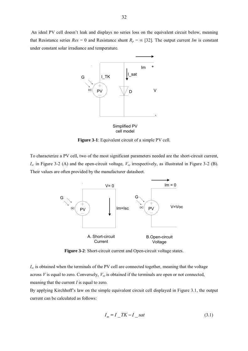
32
An ideal PV cell doesn’t leak and displays no series loss on the equivalent circuit below, meaning
that Resistance series Res = 0 and Resistance shunt Rp = ∞ [32]. The output current Im is constant
under constant solar irradiance and temperature.
DC PV
Im
G
Simplified PV cell model
I_TK
D
+
-
V
I_sat
Figure 3-1: Equivalent circuit of a simple PV cell.
To characterize a PV cell, two of the most significant parameters needed are the short-circuit current,
Isc in Figure 3-2 (A) and the open-circuit voltage, Voc irrespectively, as illustrated in Figure 3-2 (B).
Their values are often provided by the manufacturer datasheet.
DC PV Im=Isc
V= 0
G
DC PV
Im = 0
G
V=Voc
A. Short-circuit Current
B.Open-circuitVoltage
Figure 3-2: Short-circuit current and Open-circuit voltage states.
Isc is obtained when the terminals of the PV cell are connected together, meaning that the voltage
across V is equal to zero. Conversely, Voc is obtained if the terminals are open or not connected,
meaning that the current I is equal to zero.
By applying Kirchhoff’s law on the simple equivalent circuit cell displayed in Figure 3.1, the output
current can be calculated as follows:
satITKIIm __ (3.1)
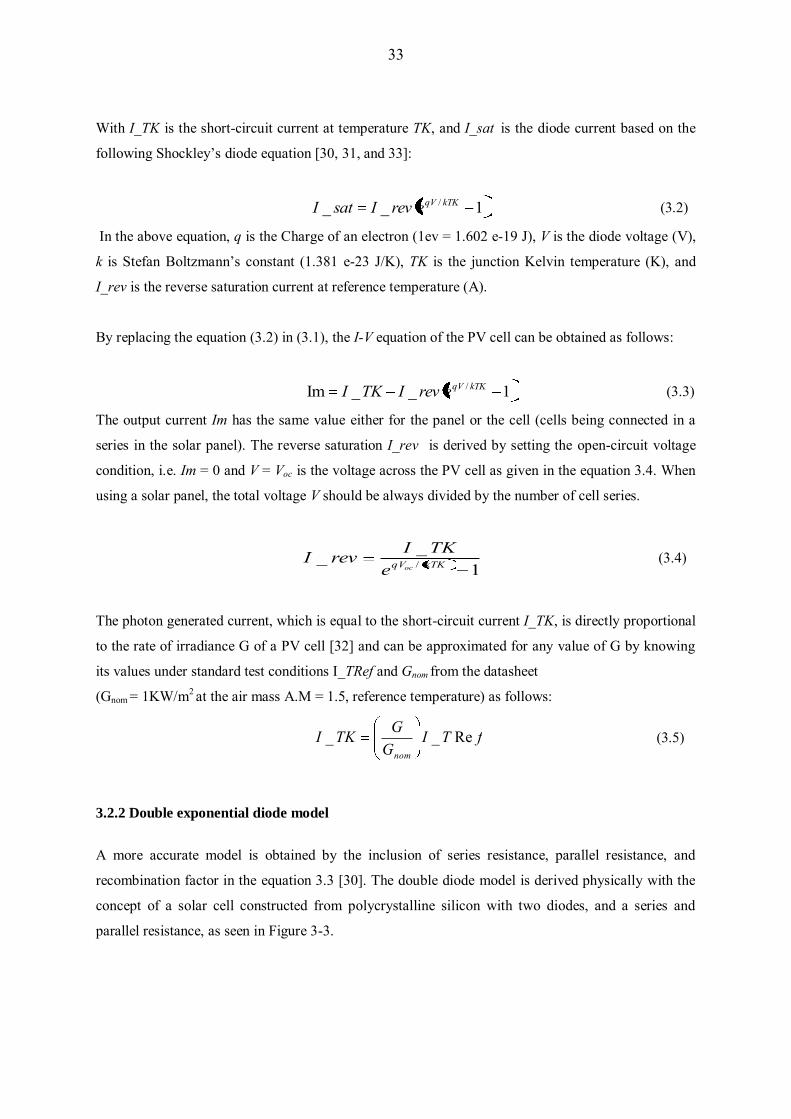
33
With I_TK is the short-circuit current at temperature TK, and I_sat is the diode current based on the
following Shockley’s diode equation [30, 31, and 33]:
1__ / kTKqVerevIsatI (3.2)
In the above equation, q is the Charge of an electron (1ev = 1.602 e-19 J), V is the diode voltage (V),
k is Stefan Boltzmann’s constant (1.381 e-23 J/K), TK is the junction Kelvin temperature (K), and
I_rev is the reverse saturation current at reference temperature (A).
By replacing the equation (3.2) in (3.1), the I-V equation of the PV cell can be obtained as follows:
1__Im / kTKqVerevITKI (3.3)
The output current Im has the same value either for the panel or the cell (cells being connected in a
series in the solar panel). The reverse saturation I_rev is derived by setting the open-circuit voltage
condition, i.e. Im = 0 and V = Voc is the voltage across the PV cell as given in the equation 3.4. When
using a solar panel, the total voltage V should be always divided by the number of cell series.
1__ / kTKqVoce
TKIrevI (3.4)
The photon generated current, which is equal to the short-circuit current I_TK, is directly proportional
to the rate of irradiance G of a PV cell [32] and can be approximated for any value of G by knowing
its values under standard test conditions I_TRef and Gnom from the datasheet
(Gnom = 1KW/m2 at the air mass A.M = 1.5, reference temperature) as follows:
fTI
GGTKInom
Re__ (3.5)
3.2.2 Double exponential diode model
A more accurate model is obtained by the inclusion of series resistance, parallel resistance, and
recombination factor in the equation 3.3 [30]. The double diode model is derived physically with the
concept of a solar cell constructed from polycrystalline silicon with two diodes, and a series and
parallel resistance, as seen in Figure 3-3.
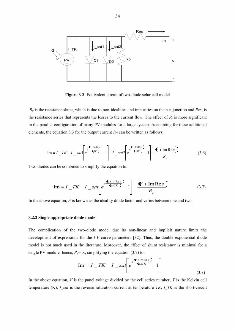
34
DC PV
Im
G I_TK
D1
+
-
V
I_sat1
D2
I_sat2
Rp
Res
Figure 3-3: Equivalent circuit of two-diode solar cell model
Rp is the resistance shunt, which is due to non-idealities and impurities on the p-n junction and Res, is
the resistance series that represents the losses to the current flow. The effect of Rp is more significant
in the parallel configuration of many PV modules for a large system. Accounting for these additional
elements, the equation 3.3 for the output current Im can be written as follows:
p
kTKsVq
kTKsVq
RsVesatIesatITKI ReIm12_11__Im 2
ReImReIm
(3.6)
Two diodes can be combined to simplify the equation to:
p
AkTKsVq
RsVesatITKI ReIm1__Im
ReIm
(3.7)
In the above equation, A is known as the ideality diode factor and varies between one and two.
3.2.3 Single appropriate diode model
The complication of the two-diode model due its non-linear and implicit nature limits the
development of expressions for the I-V curve parameters [32]. Thus, the double exponential diode
model is not much used in the literature. Moreover, the effect of shunt resistance is minimal for a
single PV module; hence, Rp= ∞, simplifying the equation (3.7) to:
1__ImReIm
AkTKsVq
esatITKI (3.8)
In the above equation, V is the panel voltage divided by the cell series number, T is the Kelvin cell
temperature (K), I_sat is the reverse saturation current at temperature TK, I_TK is the short-circuit

35
current at TK from the generator PV cell, Res is the resistance inside each cell and between the cell’s
connections and Im is the output module current, which is also the cell current.
The single diode model as displayed in Figure 3-4 includes a series resistance Res, one diode, and an
irradiance-induced current source. I_TK is the current source, which shows the current generated by a
PV cell, and its output is constant, with no variations in irradiance G and temperature T.
DC PV
Im
G I_TK
D
+
-
V
I_sat
Res
Figure 3-4: Equivalent circuit of one diode solar cell.
3.2.3.1 Matlab PV Cell model
According to Figure 3-4, the PV output panel current is directly proportional to the current falling on
solar PV cell, which in turn is also proportional to the irradiance level. The equations that show the I-
V curves of PV cell model are provided on pages [30, 31, 34 and 35] and can be resumed as follows:
1ReIm
__AkTK
sVq
satm eITKII (3.9)
))Re(1)(1( ___ fTTKalphaTTKITKI (3.10)
fTIG
GTTKInom
Re_)1( (3.11)
12
)1(_)2(_TT
TTKITTKIalpha (3.12)
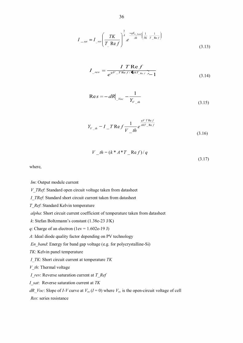
36
fTTKAkqE
A
revsat
bandn
efT
TKII Re_11
3
__
_
.Re
_ (3.13)
1Re
Re_/Re__
_ fAkTfTqVrev efTI
I (3.14)
thVVoc Y
dRs_
_
1Re (3.15)
fAkTfTqV
thV ethV
fTIY Re_Re
_
_
_1Re_
(3.16)
qfTAkthV /)Re_**(_
(3.17) where,
Im: Output module current
V_TRef: Standard open circuit voltage taken from datasheet
I_TRef: Standard short circuit current taken from datasheet
T_Ref: Standard Kelvin temperature
alpha: Short circuit current coefficient of temperature taken from datasheet
k: Stefan Boltzmann’s constant (1.38e-23 J/K)
q: Charge of an electron (1ev = 1.602e-19 J)
A: Ideal diode quality factor depending on PV technology
En_band: Energy for band gap voltage (e.g. for polycrystalline-Si)
TK: Kelvin panel temperature
I_TK: Short circuit current at temperature TK
V_th: Thermal voltage
I_rev: Reverse saturation current at T_Ref
I_sat: Reverse saturation current at TK
dR_Voc: Slope of I-V curve at Voc (I = 0) where Voc is the open-circuit voltage of cell
Res: series resistance
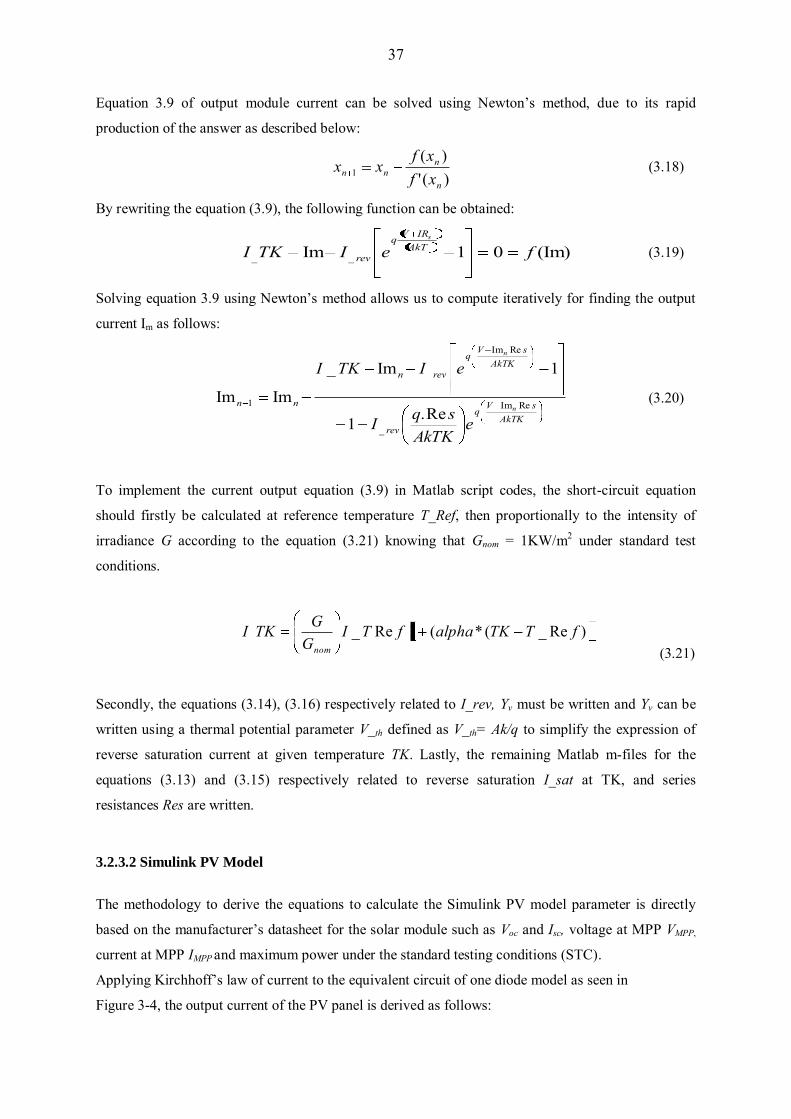
37
Equation 3.9 of output module current can be solved using Newton’s method, due to its rapid
production of the answer as described below:
)(')(
1n
nnn xf
xfxx (3.18)
By rewriting the equation (3.9), the following function can be obtained:
(Im)01Im __ feITKI AkTIRVq
rev
s
(3.19)
Solving equation 3.9 using Newton’s method allows us to compute iteratively for finding the output
current Im as follows:
AkTK
sVq
rev
AkTKsV
q
revn
nnn
n
eAkTK
sqI
eITKI
ReIm
_
ReIm
1Re.1
1Im_
ImIm (3.20)
To implement the current output equation (3.9) in Matlab script codes, the short-circuit equation
should firstly be calculated at reference temperature T_Ref, then proportionally to the intensity of
irradiance G according to the equation (3.21) knowing that Gnom = 1KW/m2 under standard test
conditions.
)Re_(*(1Re_ fTTKalphafTI
GGTKInom (3.21)
Secondly, the equations (3.14), (3.16) respectively related to I_rev, Yv must be written and Yv can be
written using a thermal potential parameter V_th defined as V_th= Ak/q to simplify the expression of
reverse saturation current at given temperature TK. Lastly, the remaining Matlab m-files for the
equations (3.13) and (3.15) respectively related to reverse saturation I_sat at TK, and series
resistances Res are written.
3.2.3.2 Simulink PV Model
The methodology to derive the equations to calculate the Simulink PV model parameter is directly
based on the manufacturer’s datasheet for the solar module such as Voc and Isc, voltage at MPP VMPP,
current at MPP IMPP and maximum power under the standard testing conditions (STC).
Applying Kirchhoff’s law of current to the equivalent circuit of one diode model as seen in
Figure 3-4, the output current of the PV panel is derived as follows:
38
satITKI __Im (3.22)
In the equation 3.22, I_TK is light current at a given temperature TK and irradiance G and can be
written as follows:
)Re_(*(Re_ fTTKalphafTI
GGTKInom (3.23)
I_sat is the reverse saturation current at TK and can be written as follows:
1__)ReIm(
kTKsVq
erevIsatI (3.24)
I_rev is the reverse saturation at a reference temperature T_Ref, δ is the ideal shape factor and is equal
to the product of ideal diode quality factor A and cell series number Ns. The output current equation
used in the Simulink model can be derived by replacing the equation 3.24 into the equation 3.22 and
this substitution results in the following equation:
1__ImReIm
kTKsVq
erevITKI (3.25)
The general equation 3.25 above has four unknown parameters I_TK, I_rev, Res, δ.
Once I_TK and I rev are known at standard condition, they can be updated for specific conditions.
Assuming that the series resistance parameter can be determined by the bisection method proposed by
Townsend [36] as follows:
refMPP
refMPPs
refMPP
VfTVfTI
Iq
fkTNI
s ,_,_
,
ReRe_
1lnRe1Re
(3.26)
NS, IMPP,ref and VMPP,ref represent the cell number, current and voltage at MPP respectively and IMPP,ref
and VMPP,ref are always given in the datasheet under STC. By knowing Res, this reduces the number of
unknowns to three I_TK, I_rev, δ. The solution can be obtained by trying to force the I-V
characteristic to pass through MPP, open, and short circuit points.
It is also known that:
Im = I_TRef at short-circuit state (V = 0)
V = V_TRef at open-circuit state (Im = 0)
Im = IMPP and V = VMPP at maximum power (MPP)
39
Firstly let’s find I_TK and I_sat at standard condition by rearranging these above expressions in the
equation (3.25).
fkTfTqVrevIrefTKIfTI
Re_)Re_(_,_Re_ (3.27)
1Re_Re_exp_,_0
fkTfTqVrevIrefTKI (3.28)
1Re_
Reexp_,_ ,,
, fkTsIqV
revIrefTKII refMPPrefMPPrefMPP (3.29)
I_rev through the diode is found to be the range of 10-5 and 10-6 due to the very small value of Res and
can be negligible [36]. This means that the short circuit and light current are equal under all
conditions. Thus, the equation 3.27 can be written as follows:
refTKIfTI ,_Re_ (3.30)
By rearranging the equations 3.27 and 3.28 together, the ideal shape factor can be deducted as:
fTIIfkT
fTVRIVq
refMPP
srefMPPrefMPP
Re_/1lnRe_Re_
,
,, (3.31)
The reverse saturation current I_rev can be deducted from the equation 3.28 and written as follows:
fV
fTIrevIRe_exp
Re__ (3.32)
where an auxiliary variable fkT
qRe_ (3.33)
The reverse saturation current at TK can now be calculated as follows:
fTTKkqE
A
revsat
bandn
efT
TKII Re_11
3
__
_
.Re
_ (3.34)
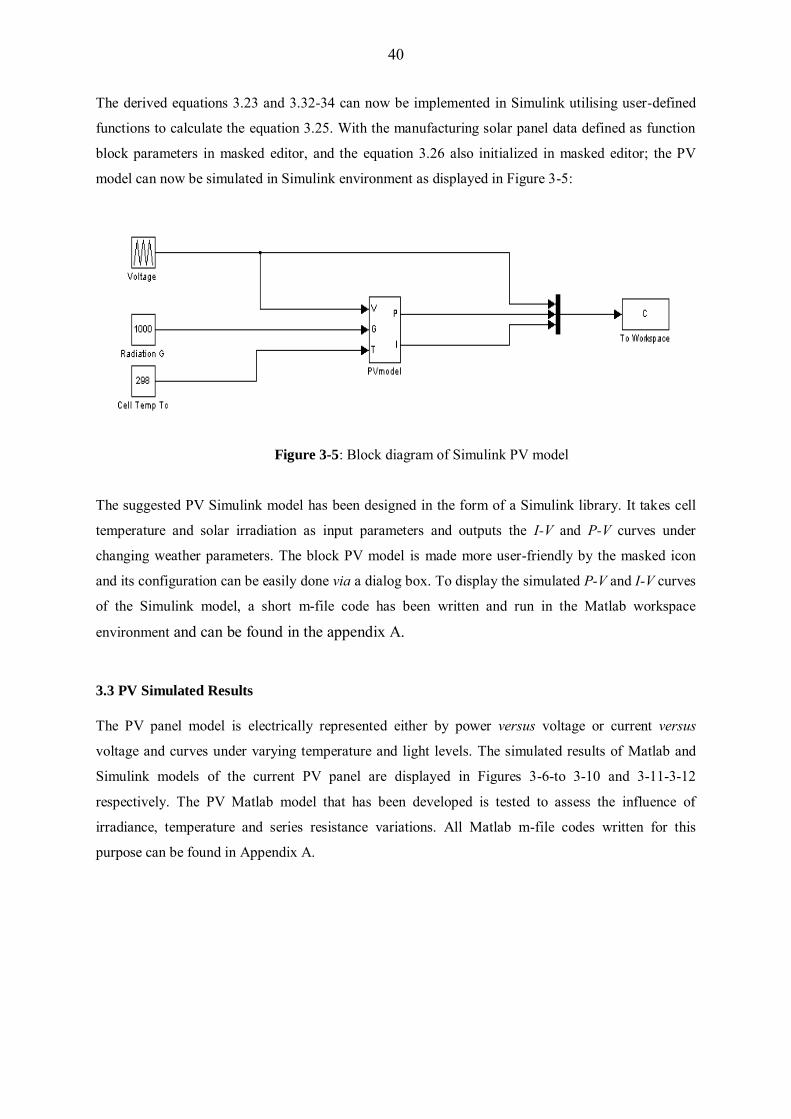
40
The derived equations 3.23 and 3.32-34 can now be implemented in Simulink utilising user-defined
functions to calculate the equation 3.25. With the manufacturing solar panel data defined as function
block parameters in masked editor, and the equation 3.26 also initialized in masked editor; the PV
model can now be simulated in Simulink environment as displayed in Figure 3-5:
Figure 3-5: Block diagram of Simulink PV model
The suggested PV Simulink model has been designed in the form of a Simulink library. It takes cell
temperature and solar irradiation as input parameters and outputs the I-V and P-V curves under
changing weather parameters. The block PV model is made more user-friendly by the masked icon
and its configuration can be easily done via a dialog box. To display the simulated P-V and I-V curves
of the Simulink model, a short m-file code has been written and run in the Matlab workspace
environment and can be found in the appendix A.
3.3 PV Simulated Results
The PV panel model is electrically represented either by power versus voltage or current versus
voltage and curves under varying temperature and light levels. The simulated results of Matlab and
Simulink models of the current PV panel are displayed in Figures 3-6-to 3-10 and 3-11-3-12
respectively. The PV Matlab model that has been developed is tested to assess the influence of
irradiance, temperature and series resistance variations. All Matlab m-file codes written for this
purpose can be found in Appendix A.
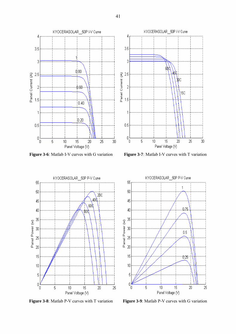
41
Figure 3-6: Matlab I-V curves with G variation Figure 3-7: Matlab I-V curves with T variation
Figure 3-8: Matlab P-V curves with T variation Figure 3-9: Matlab P-V curves with G variation
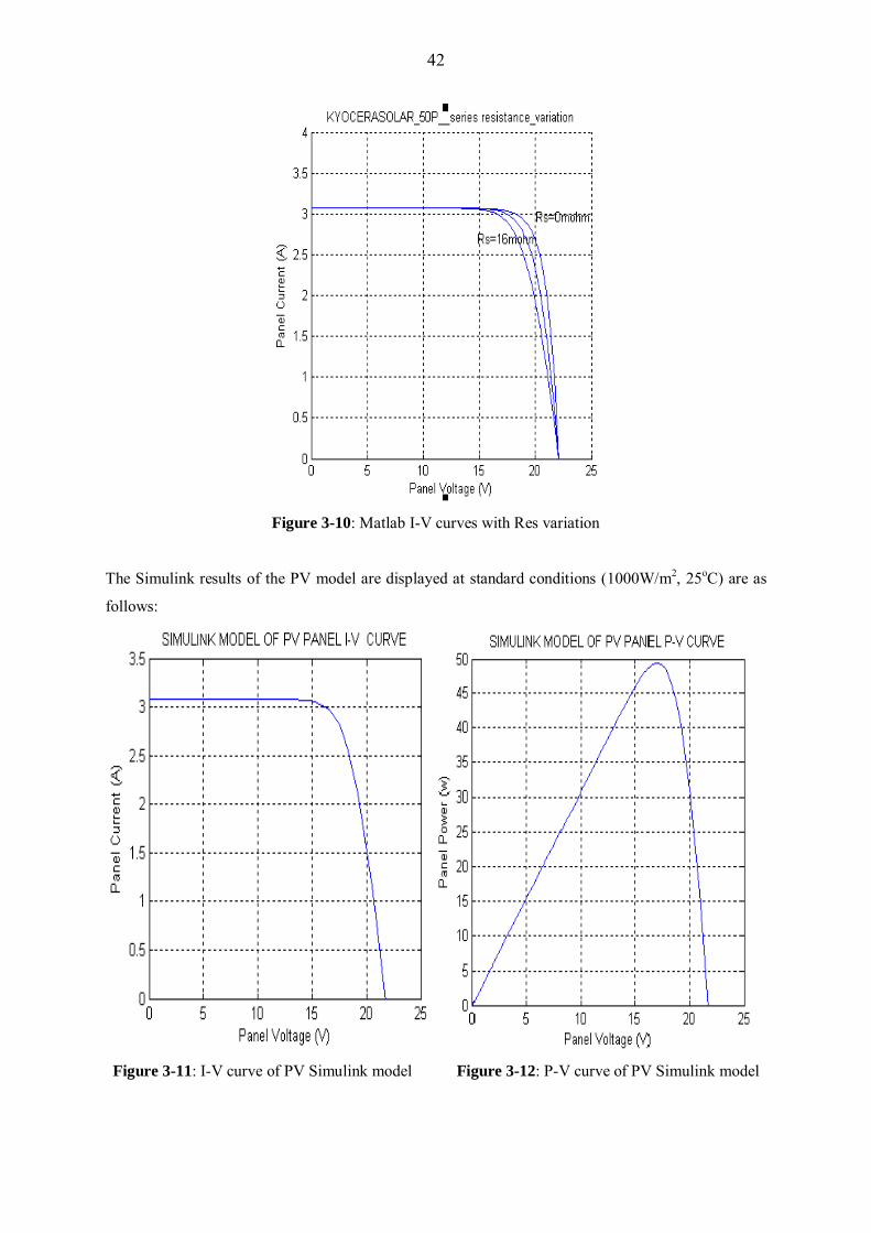
42
Figure 3-10: Matlab I-V curves with Res variation
The Simulink results of the PV model are displayed at standard conditions (1000W/m2, 25oC) are as
follows:
Figure 3-11: I-V curve of PV Simulink model Figure 3-12: P-V curve of PV Simulink model
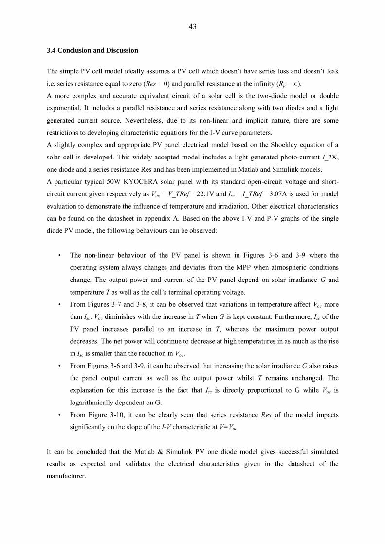
43
3.4 Conclusion and Discussion
The simple PV cell model ideally assumes a PV cell which doesn’t have series loss and doesn’t leak
i.e. series resistance equal to zero (Res = 0) and parallel resistance at the infinity (Rp = ∞).
A more complex and accurate equivalent circuit of a solar cell is the two-diode model or double
exponential. It includes a parallel resistance and series resistance along with two diodes and a light
generated current source. Nevertheless, due to its non-linear and implicit nature, there are some
restrictions to developing characteristic equations for the I-V curve parameters.
A slightly complex and appropriate PV panel electrical model based on the Shockley equation of a
solar cell is developed. This widely accepted model includes a light generated photo-current I_TK,
one diode and a series resistance Res and has been implemented in Matlab and Simulink models.
A particular typical 50W KYOCERA solar panel with its standard open-circuit voltage and short-
circuit current given respectively as Voc = V_TRef = 22.1V and Isc = I_TRef = 3.07A is used for model
evaluation to demonstrate the influence of temperature and irradiation. Other electrical characteristics
can be found on the datasheet in appendix A. Based on the above I-V and P-V graphs of the single
diode PV model, the following behaviours can be observed:
• The non-linear behaviour of the PV panel is shown in Figures 3-6 and 3-9 where the
operating system always changes and deviates from the MPP when atmospheric conditions
change. The output power and current of the PV panel depend on solar irradiance G and
temperature T as well as the cell’s terminal operating voltage.
• From Figures 3-7 and 3-8, it can be observed that variations in temperature affect Voc more
than Isc. Voc diminishes with the increase in T when G is kept constant. Furthermore, Isc of the
PV panel increases parallel to an increase in T, whereas the maximum power output
decreases. The net power will continue to decrease at high temperatures in as much as the rise
in Isc is smaller than the reduction in Voc.
• From Figures 3-6 and 3-9, it can be observed that increasing the solar irradiance G also raises
the panel output current as well as the output power whilst T remains unchanged. The
explanation for this increase is the fact that Isc is directly proportional to G while Voc is
logarithmically dependent on G.
• From Figure 3-10, it can be clearly seen that series resistance Res of the model impacts
significantly on the slope of the I-V characteristic at V=Voc.
It can be concluded that the Matlab & Simulink PV one diode model gives successful simulated
results as expected and validates the electrical characteristics given in the datasheet of the
manufacturer.

44
Chapter 4: MAXIMUM POWER POINT TRACKING ALGORITHM
MODELS
4.0 Introduction
All the MPPT algorithms have been investigated with actual irradiance data provided by the South
African Weather Service (SAWS) [37]. Using SAWS data, a text-file containing the Kipp and Zonen
pyranometer data of radiation intensity is found on a horizontal surface in the meteorological wavelength
band, i.e. Lamda = 0.3 to 2.8 microns. Hourly solar global radiation for 24 hours of local apparent time is
measured in kilojoules per square metres per hour. Two sets of data are used in the current simulation
study. Both contain useful and different weather measurements taken in Upington, South Africa.
A sunny data measurement is taken on 6 February 1966 and a cloudy data measurement is taken on 11
January 1966. These historic data are accurate and still reliable. They include the irradiation
measurements taken each hour for 24 hours as seen in appendix B. The linear interpolations in Matlab
functions are useful to estimate the irradiance values between two hourly data points. The solar data is
displayed in Figure 4-1; it can be observed, on the one hand, that the irradiance intensity varies little
during a sunny day due to the lack passing clouds. Therefore MPP tracking is smooth and not
challenging. On the other hand, MPP tracking seems to be cumbersome on a cloudy day because the
irradiance intensity varies abruptly due to passing clouds. A specific MPPT algorithm may perform better
in one environmental situation and fail to track well in another, or may also outperform another algorithm
under the same operating weather conditions. Therefore, it is crucial to define a parameter called
“tracking efficiency” in order to establish the performance of a given MPPT algorithm and to be able to
make comparisons with other MPPT algorithms. A modeling and simulation study is presented in the
following section to compare the performance of the MPPT algorithms under sunny and cloudy weather
scenarios.
Based on the literature review, the classical low-cost and widely used PO and IC MPPT algorithms are
selected, and written in Matlab m-files and simulated. Some of their optimized solutions for improved
performance are also investigated. These include the PO modified version 1(MPO), PO modified version
2 (EPP), and an improved two-stage algorithm combining modified CV and IC methods [20, 25].
However, some minor modifications are introduced in the improved two-mode algorithm by removing the
expensive sensor device used for the measurement of radiation. Moreover, the converter duty cycle is
used as a control variable, simplifying the MPPT system in one direct control loop during its
implementation in the whole PV system Simulink model.
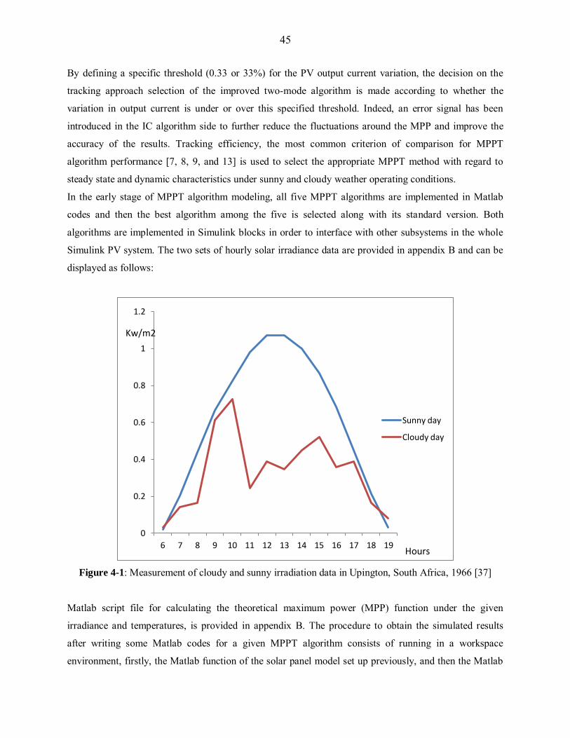
45
By defining a specific threshold (0.33 or 33%) for the PV output current variation, the decision on the
tracking approach selection of the improved two-mode algorithm is made according to whether the
variation in output current is under or over this specified threshold. Indeed, an error signal has been
introduced in the IC algorithm side to further reduce the fluctuations around the MPP and improve the
accuracy of the results. Tracking efficiency, the most common criterion of comparison for MPPT
algorithm performance [7, 8, 9, and 13] is used to select the appropriate MPPT method with regard to
steady state and dynamic characteristics under sunny and cloudy weather operating conditions.
In the early stage of MPPT algorithm modeling, all five MPPT algorithms are implemented in Matlab
codes and then the best algorithm among the five is selected along with its standard version. Both
algorithms are implemented in Simulink blocks in order to interface with other subsystems in the whole
Simulink PV system. The two sets of hourly solar irradiance data are provided in appendix B and can be
displayed as follows:
Figure 4-1: Measurement of cloudy and sunny irradiation data in Upington, South Africa, 1966 [37]
Matlab script file for calculating the theoretical maximum power (MPP) function under the given
irradiance and temperatures, is provided in appendix B. The procedure to obtain the simulated results
after writing some Matlab codes for a given MPPT algorithm consists of running in a workspace
environment, firstly, the Matlab function of the solar panel model set up previously, and then the Matlab
0
0.2
0.4
0.6
0.8
1
1.2
6 7 8 9 10 11 12 13 14 15 16 17 18 19
Sunny day
Cloudy day
Kw/m2
Hours
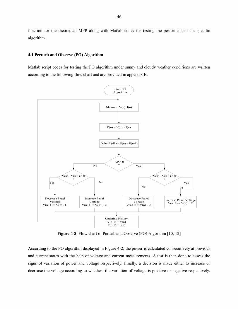
46
function for the theoretical MPP along with Matlab codes for testing the performance of a specific
algorithm.
4.1 Perturb and Observe (PO) Algorithm
Matlab script codes for testing the PO algorithm under sunny and cloudy weather conditions are written
according to the following flow chart and are provided in appendix B.
∆P > 0?
V(n) - V(n-1) > 0 ?
V(n) - V(n-1) > 0?
Decrease Panel Voltage
V(n+1) = V(n) - C
Increase Panel Voltage
V(n+1) = V(n) + C
Decrease Panel Voltage
V(n+1) = V(n) - C
Increase Panel VoltageV(n+1) = V(n) + C
Updating HistoryV(n-1) = V(n)P(n-1) = P(n)
Delta P (dP) = P(n) – P(n-1)
P(n) = V(n) x I(n)
Measure: V(n), I(n)
No
Start PO Algorithm
No YesYes
No Yes
Figure 4-2: Flow chart of Perturb and Observe (PO) Algorithm [10, 12]
According to the PO algorithm displayed in Figure 4-2, the power is calculated consecutively at previous
and current states with the help of voltage and current measurements. A test is then done to assess the
signs of variation of power and voltage respectively. Finally, a decision is made either to increase or
decrease the voltage according to whether the variation of voltage is positive or negative respectively.
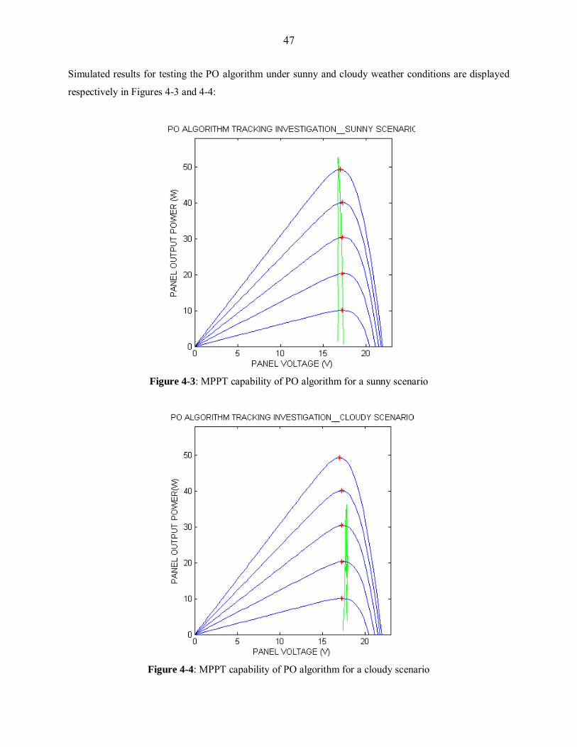
47
Simulated results for testing the PO algorithm under sunny and cloudy weather conditions are displayed
respectively in Figures 4-3 and 4-4:
Figure 4-3: MPPT capability of PO algorithm for a sunny scenario
Figure 4-4: MPPT capability of PO algorithm for a cloudy scenario
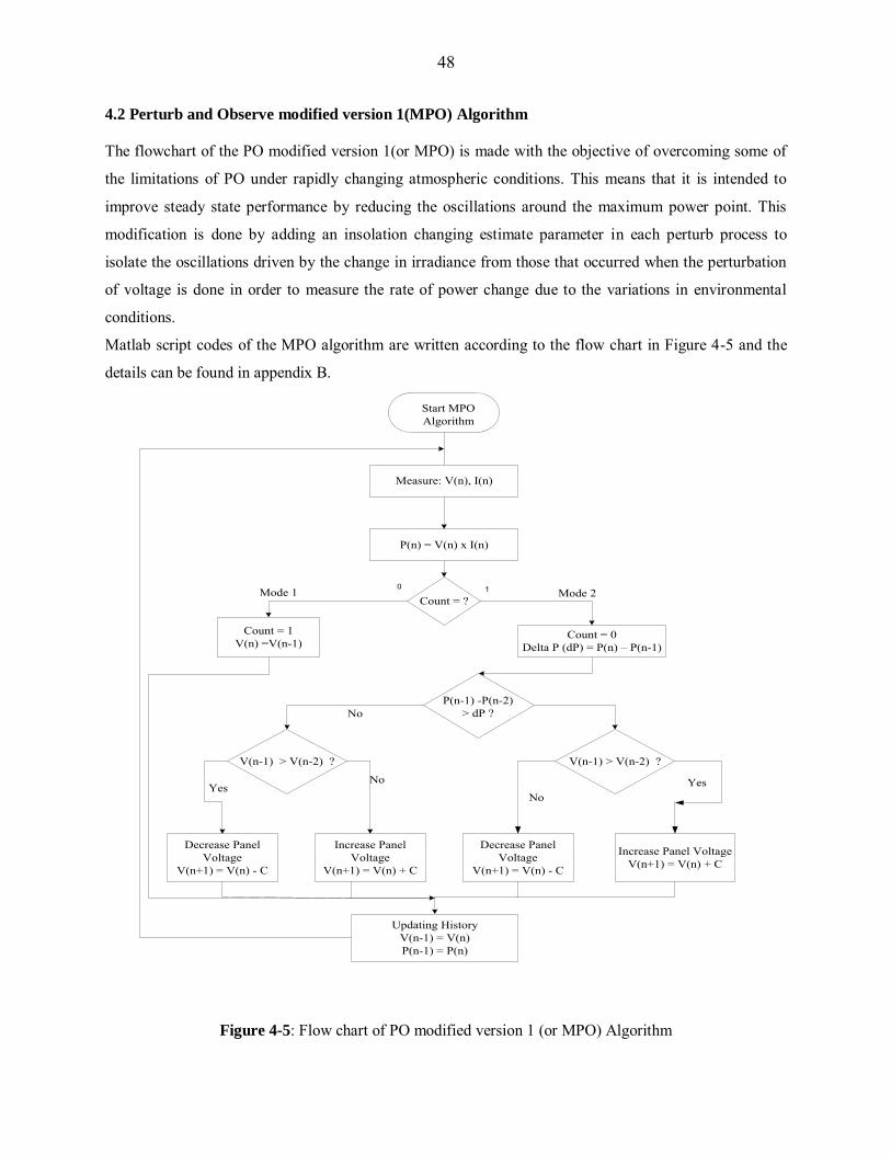
48
4.2 Perturb and Observe modified version 1(MPO) Algorithm
The flowchart of the PO modified version 1(or MPO) is made with the objective of overcoming some of
the limitations of PO under rapidly changing atmospheric conditions. This means that it is intended to
improve steady state performance by reducing the oscillations around the maximum power point. This
modification is done by adding an insolation changing estimate parameter in each perturb process to
isolate the oscillations driven by the change in irradiance from those that occurred when the perturbation
of voltage is done in order to measure the rate of power change due to the variations in environmental
conditions.
Matlab script codes of the MPO algorithm are written according to the flow chart in Figure 4-5 and the
details can be found in appendix B.
P(n-1) -P(n-2) > dP ?
V(n-1) > V(n-2) ?V(n-1) > V(n-2) ?
Decrease Panel Voltage
V(n+1) = V(n) - C
Increase Panel Voltage
V(n+1) = V(n) + C
Decrease Panel Voltage
V(n+1) = V(n) - C
Increase Panel VoltageV(n+1) = V(n) + C
Updating HistoryV(n-1) = V(n)P(n-1) = P(n)
Count = 0Delta P (dP) = P(n) – P(n-1)
P(n) = V(n) x I(n)
Measure: V(n), I(n)
No
Start MPO Algorithm
No YesYes
No
Count = 1V(n) =V(n-1)
Count = ?Mode 2Mode 1
0 1
Figure 4-5: Flow chart of PO modified version 1 (or MPO) Algorithm
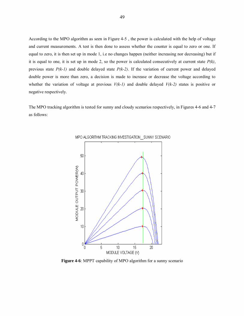
49
According to the MPO algorithm as seen in Figure 4-5 , the power is calculated with the help of voltage
and current measurements. A test is then done to assess whether the counter is equal to zero or one. If
equal to zero, it is then set up in mode 1, i.e no changes happen (neither increasing nor decreasing) but if
it is equal to one, it is set up in mode 2, so the power is calculated consecutively at current state P(k),
previous state P(k-1) and double delayed state P(k-2). If the variation of current power and delayed
double power is more than zero, a decision is made to increase or decrease the voltage according to
whether the variation of voltage at previous V(k-1) and double delayed V(k-2) states is positive or
negative respectively.
The MPO tracking algorithm is tested for sunny and cloudy scenarios respectively, in Figures 4-6 and 4-7
as follows:
Figure 4-6: MPPT capability of MPO algorithm for a sunny scenario
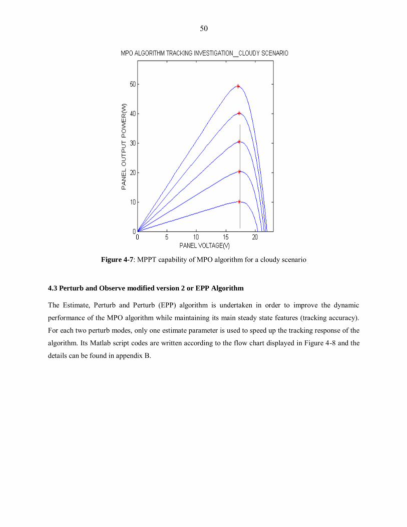
50
Figure 4-7: MPPT capability of MPO algorithm for a cloudy scenario
4.3 Perturb and Observe modified version 2 or EPP Algorithm
The Estimate, Perturb and Perturb (EPP) algorithm is undertaken in order to improve the dynamic
performance of the MPO algorithm while maintaining its main steady state features (tracking accuracy).
For each two perturb modes, only one estimate parameter is used to speed up the tracking response of the
algorithm. Its Matlab script codes are written according to the flow chart displayed in Figure 4-8 and the
details can be found in appendix B.
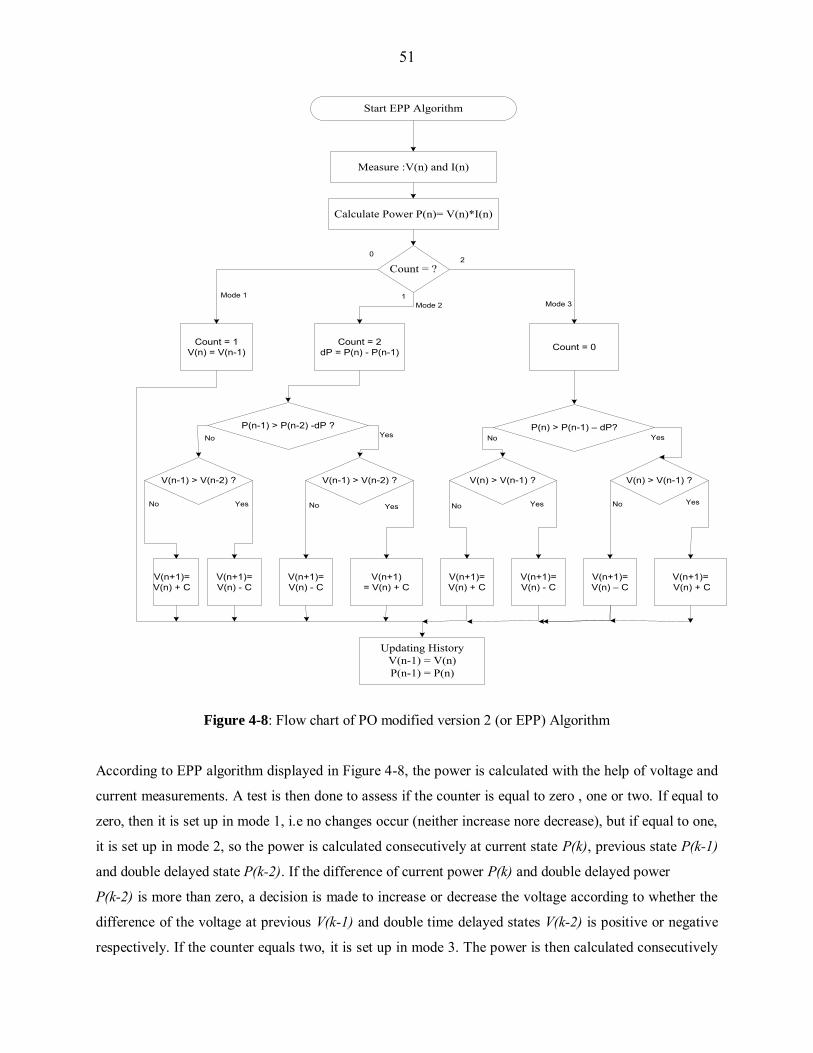
51
V(n+1)= V(n) - C
V(n+1)= V(n) - C
V(n+1)= V(n) + C
V(n+1)= V(n) + C
V(n+1)= V(n) - C
V(n+1)= V(n) – C
V(n+1)= V(n) + C
V(n+1)= V(n) + C
V(n-1) > V(n-2) ? V(n-1) > V(n-2) ? V(n) > V(n-1) ? V(n) > V(n-1) ?
P(n-1) > P(n-2) -dP ? P(n) > P(n-1) – dP?
Count = 1V(n) = V(n-1)
Count = 2dP = P(n) - P(n-1) Count = 0
Count = ?
Calculate Power P(n)= V(n)*I(n)
Measure :V(n) and I(n)
Start EPP Algorithm
Updating HistoryV(n-1) = V(n)P(n-1) = P(n)
0
1
2
Mode 1Mode 2 Mode 3
No Yes No Yes No Yes No Yes
No Yes No Yes
Figure 4-8: Flow chart of PO modified version 2 (or EPP) Algorithm
According to EPP algorithm displayed in Figure 4-8, the power is calculated with the help of voltage and
current measurements. A test is then done to assess if the counter is equal to zero , one or two. If equal to
zero, then it is set up in mode 1, i.e no changes occur (neither increase nore decrease), but if equal to one,
it is set up in mode 2, so the power is calculated consecutively at current state P(k), previous state P(k-1)
and double delayed state P(k-2). If the difference of current power P(k) and double delayed power
P(k-2) is more than zero, a decision is made to increase or decrease the voltage according to whether the
difference of the voltage at previous V(k-1) and double time delayed states V(k-2) is positive or negative
respectively. If the counter equals two, it is set up in mode 3. The power is then calculated consecutively
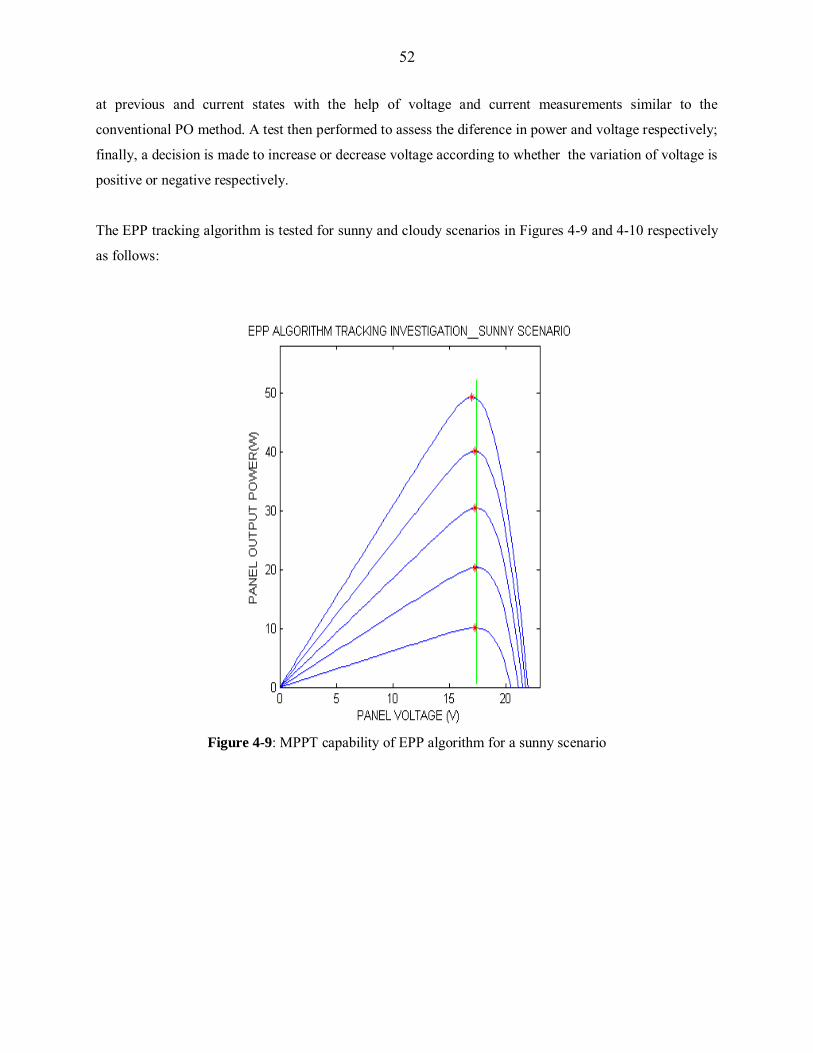
52
at previous and current states with the help of voltage and current measurements similar to the
conventional PO method. A test then performed to assess the diference in power and voltage respectively;
finally, a decision is made to increase or decrease voltage according to whether the variation of voltage is
positive or negative respectively.
The EPP tracking algorithm is tested for sunny and cloudy scenarios in Figures 4-9 and 4-10 respectively
as follows:
Figure 4-9: MPPT capability of EPP algorithm for a sunny scenario
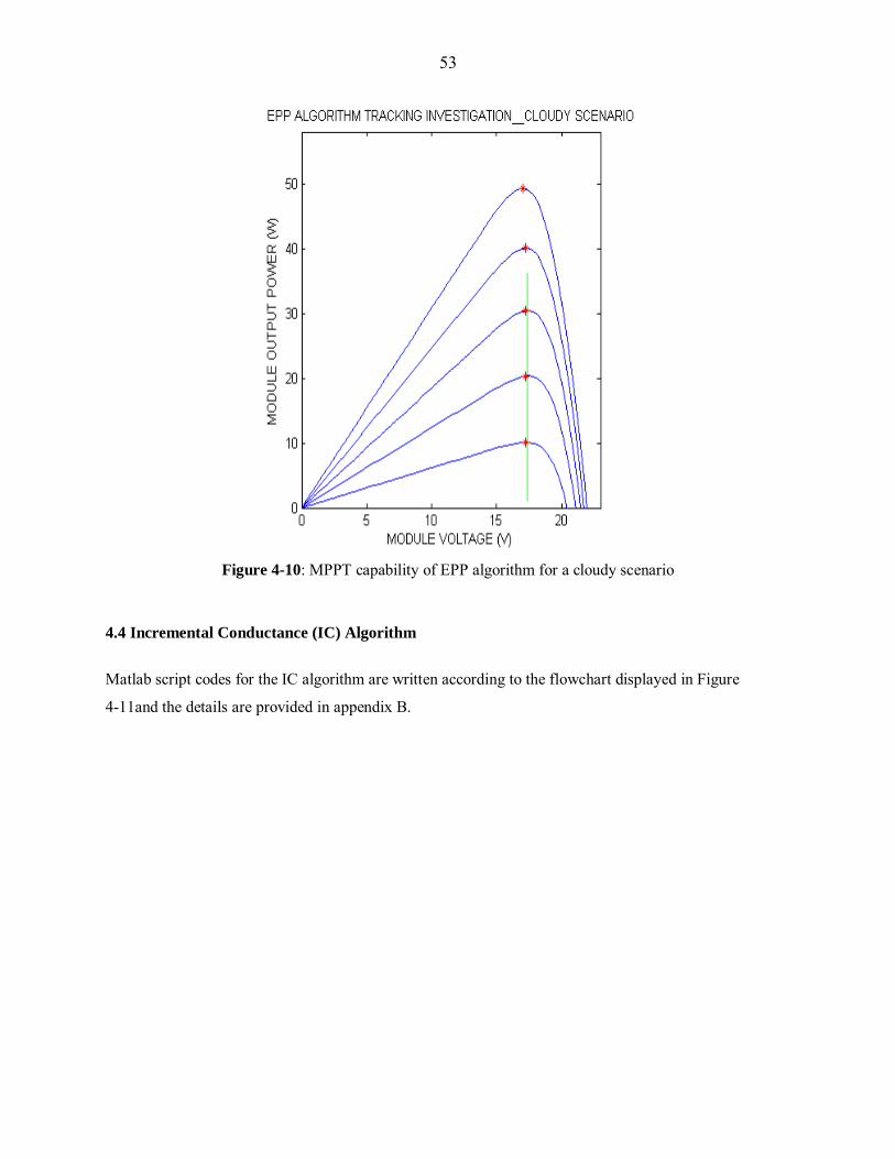
53
Figure 4-10: MPPT capability of EPP algorithm for a cloudy scenario
4.4 Incremental Conductance (IC) Algorithm
Matlab script codes for the IC algorithm are written according to the flowchart displayed in Figure
4-11and the details are provided in appendix B.
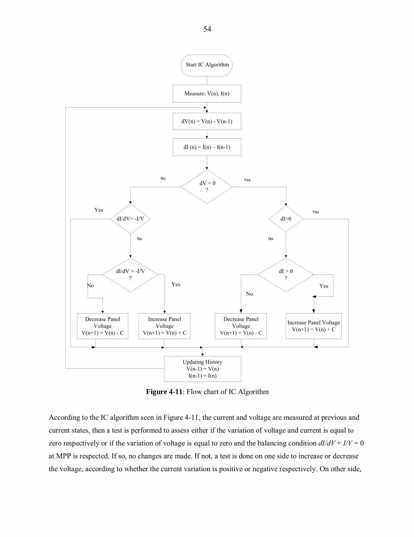
54
dV = 0?
dI > 0 ?
dI/dV > -I/V?
Decrease Panel Voltage
V(n+1) = V(n) - C
Increase Panel Voltage
V(n+1) = V(n) + C
Decrease Panel Voltage
V(n+1) = V(n) - C
Increase Panel VoltageV(n+1) = V(n) + C
Updating HistoryV(n-1) = V(n)I(n-1) = I(n)
dI (n) = I(n) – I(n-1)
dV(n) = V(n) - V(n-1)
Measure: V(n), I(n)
No
Start IC Algorithm
Yes YesNo
dI/dV= -I/V dI=0
YesNo
Yes Yes
NoNo
Figure 4-11: Flow chart of IC Algorithm
According to the IC algorithm seen in Figure 4-11, the current and voltage are measured at previous and
current states, then a test is performed to assess either if the variation of voltage and current is equal to
zero respectively or if the variation of voltage is equal to zero and the balancing condition dI/dV + I/V = 0
at MPP is respected. If so, no changes are made. If not, a test is done on one side to increase or decrease
the voltage, according to whether the current variation is positive or negative respectively. On other side,
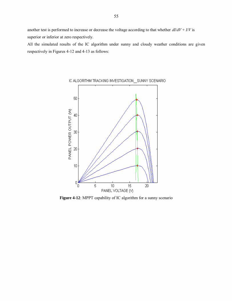
55
another test is performed to increase or decrease the voltage according to that whether dI/dV + I/V is
superior or inferior at zero respectively.
All the simulated results of the IC algorithm under sunny and cloudy weather conditions are given
respectively in Figures 4-12 and 4-13 as follows:
Figure 4-12: MPPT capability of IC algorithm for a sunny scenario
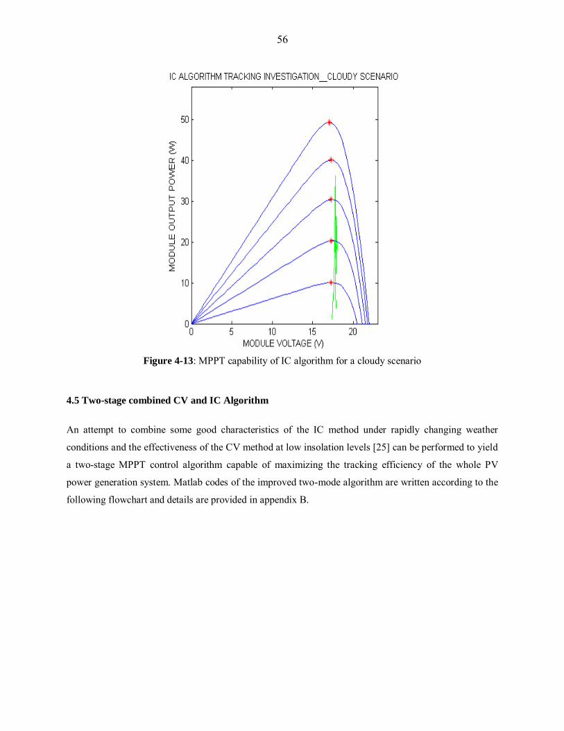
56
Figure 4-13: MPPT capability of IC algorithm for a cloudy scenario
4.5 Two-stage combined CV and IC Algorithm
An attempt to combine some good characteristics of the IC method under rapidly changing weather
conditions and the effectiveness of the CV method at low insolation levels [25] can be performed to yield
a two-stage MPPT control algorithm capable of maximizing the tracking efficiency of the whole PV
power generation system. Matlab codes of the improved two-mode algorithm are written according to the
following flowchart and details are provided in appendix B.
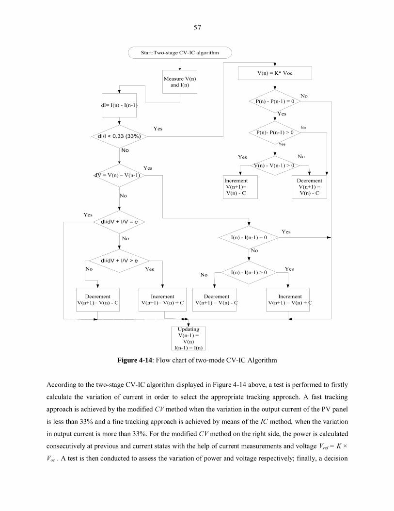
57
Start:Two-stage CV-IC algorithm
DecrementV(n+1)= V(n) - C
IncrementV(n+1)= V(n) + C
DecrementV(n+1) = V(n) - C
Increment V(n+1) = V(n) + C
UpdatingV(n-1) =
V(n)I(n-1) = I(n)
dI/dV + I/V > e
dI/dV + I/V = e
I(n) - I(n-1) > 0
I(n) - I(n-1) = 0
dV = V(n) – V(n-1)
dI/I < 0.33 (33%)
Measure V(n) and I(n)
P(n) - P(n-1) = 0
P(n)- P(n-1) > 0
V(n) - V(n-1) > 0
IncrementV(n+1)= V(n) - C
DecrementV(n+1) = V(n) - C
V(n) = K* Voc
dI= I(n) - I(n-1)
No
Yes
Yes
No
No
Yes
No YesNo
Yes
Yes No
Yes
No
No
No
Yes
Yes
Figure 4-14: Flow chart of two-mode CV-IC Algorithm
According to the two-stage CV-IC algorithm displayed in Figure 4-14 above, a test is performed to firstly
calculate the variation of current in order to select the appropriate tracking approach. A fast tracking
approach is achieved by the modified CV method when the variation in the output current of the PV panel
is less than 33% and a fine tracking approach is achieved by means of the IC method, when the variation
in output current is more than 33%. For the modified CV method on the right side, the power is calculated
consecutively at previous and current states with the help of current measurements and voltage Vref = K ×
Voc . A test is then conducted to assess the variation of power and voltage respectively; finally, a decision
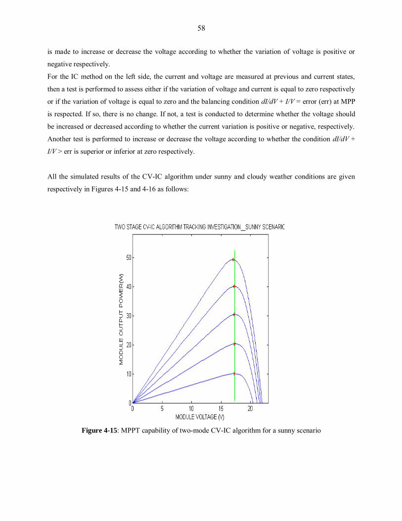
58
is made to increase or decrease the voltage according to whether the variation of voltage is positive or
negative respectively.
For the IC method on the left side, the current and voltage are measured at previous and current states,
then a test is performed to assess either if the variation of voltage and current is equal to zero respectively
or if the variation of voltage is equal to zero and the balancing condition dI/dV + I/V = error (err) at MPP
is respected. If so, there is no change. If not, a test is conducted to determine whether the voltage should
be increased or decreased according to whether the current variation is positive or negative, respectively.
Another test is performed to increase or decrease the voltage according to whether the condition dI/dV +
I/V > err is superior or inferior at zero respectively.
All the simulated results of the CV-IC algorithm under sunny and cloudy weather conditions are given
respectively in Figures 4-15 and 4-16 as follows:
Figure 4-15: MPPT capability of two-mode CV-IC algorithm for a sunny scenario
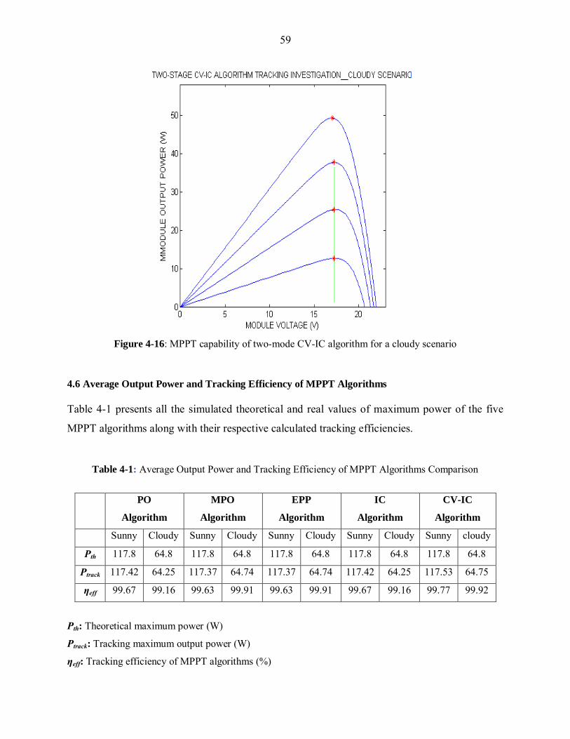
59
Figure 4-16: MPPT capability of two-mode CV-IC algorithm for a cloudy scenario
4.6 Average Output Power and Tracking Efficiency of MPPT Algorithms
Table 4-1 presents all the simulated theoretical and real values of maximum power of the five
MPPT algorithms along with their respective calculated tracking efficiencies.
Table 4-1: Average Output Power and Tracking Efficiency of MPPT Algorithms Comparison
PO
Algorithm
MPO
Algorithm
EPP
Algorithm
IC
Algorithm
CV-IC
Algorithm
Sunny Cloudy Sunny Cloudy Sunny Cloudy Sunny Cloudy Sunny cloudy
Pth 117.8 64.8 117.8 64.8 117.8 64.8 117.8 64.8 117.8 64.8
Ptrack 117.42 64.25 117.37 64.74 117.37 64.74 117.42 64.25 117.53 64.75
ηeff 99.67 99.16 99.63 99.91 99.63 99.91 99.67 99.16 99.77 99.92
Pth: Theoretical maximum power (W)
Ptrack: Tracking maximum output power (W)
ηeff: Tracking efficiency of MPPT algorithms (%)

60
4.7 Discussion and Analysis
Figures 4-3 and 4-12 illustrate that both conventional PO and IC methods perform better under sunny
conditions but when abrupt solar irradiances occur, more perturbations happen around MPP, increasing
power losses in the PV system, so that it becomes difficult to maintain the operating point at MPP. As it
can be seen in Figures 4-4 and 4-13, the trace of operating tracking power coloured in green move away
from the maximum power MPP due to the increase in power fluctuations. This justifies the theory in the
current literature, which declares that classical MPPT algorithms cannot accommodate both a good steady
state and fast transient response simultaneously; there is always a tradeoff between high accuracy (low
power fluctuations) and a fast response to dynamic changes in atmospheric conditions. All the improved
MPPT algorithms (MPO, EPP, and CV-IC) perform much better under sunny and cloudy weather
conditions compared to the standard PO and IC methods, but the two-stage CV-IC method outperforms
the MPO and EPP methods as demonstrated by its average output power and higher tracking efficiencies
for both scenarios, especially when solar irradiance is changing rapidly (a cloudy scenario). It can
simultaneously accommodate a fast responding speed and satisfactory tracking accuracy, which can
significantly diminish the energy losses that occur when clouds pass over. Because the fast and fine
tracking approaches are separately implemented in this improved method, the perturbation step size can
be set very small, which is different from the standard IC method, where the width step size should be
able to simultaneously meet simultaneously accuracy and tracking speed requirements.
The two-mode modified CV-IC is therefore selected from the five algorithms for later implementation in
the whole Simulink PV system.
Moreover, when compared to the experimental and simulated results of MPPT algorithms found in the
literature [3, 6, 7, 8, 11, 13, 33, 38], this MPPT simulation study provides meaningful and acceptable
results, which are quite close to previously published findings.
61
Chapter 5: DC-DC CONVERTER TOPOLOGY AND INTERFACE
ANALYSIS
5.1 Switch-Mode Converter Theory
Electronic power devices such as switch-mode converters are needed to reduce power losses as
much as possible, and to deliver and distribute power efficiently. They may be applicable to
interface with the PV system in order to extract the maximum power from the PV panel and
reduce the power losses that occur in direct coupled PV-load systems. A switch-mode converter
consists of inductors, capacitors, and switches. These electronic power semiconductor switches
are used in on and off states.
Switching converters are considered ideal components and yield high efficiencies. Their
switching operation is achieved by means of a power switch, often a Mosfet, which switches on
and off as soon it receives driving square wave signals at its gate. The power dissipates and
moves towards zero when the mosfet is in the off position because the current is zero. Similarly,
the power dissipates and converges towards zero in a saturated situation, because at this point in
time the voltage has dropped to near to zero [39]. The operation of the DC-DC converter consists
of two different modes: the Continuous Conduction Mode (CCM) and the Discontinuous
Conduction Mode (DCM).
A switching converter is said to be operating in CCM, if the inductor current cannot reach zero in
one switching cycle and in DCM, if the inductor current reaches zero before the end of one
switching cycle and remains there for certain period of time [39].
When the converter operates, the mosfet will be closed and open at constant frequency fs for a
certain amount of time through a method called pulse width modulation (PWM), which allows
one to control and regulate the output voltage. This control method PWM employs the switch
duty ratio D, which is the ratio of on-time ton of DTs, to the total time duration of the switching
period Ts = ton + toff as seen in Figure 5-1.
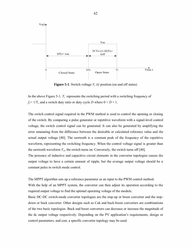
62
0 DTs Ts
DTs= tonD’Ts=(1-D)Ts=
toff
Vs(t)
Vm
Time tClosed State Open State
Figure 5-1: Switch voltage Vs (t) position (on and off states)
In the above Figure 5-1, Ts represents the switching period with a switching frequency of
fs = 1/Ts and a switch duty ratio or duty cycle D where 0 < D < 1.
The switch control signal required in the PWM method is used to control the opening or closing
of the switch. By comparing a pulse generator or repetitive waveform with a signal-level control
voltage, the switch control signal can be generated. It can also be generated by amplifying the
error emanating from the difference between the desirable or calculated reference value and the
actual output voltage [40]. The sawtooth is a constant peak of the frequency of the repetitive
waveform, representing the switching frequency. When the control voltage signal is greater than
the sawtooth waveform Vst, the switch turns on. Conversely, the switch turns off [40].
The presence of inductive and capacitive circuit elements in the converter topologies causes the
output voltage to have a certain amount of ripple, but the average output voltage should be a
constant pulse in switch mode control.
The MPPT algorithm sets up a reference parameter as an input to the PWM control method.
With the help of an MPPT system, the converter can then adjust its operation according to the
required output voltage to find the optimal operating voltage of the module.
Basic DC-DC switch-mode converter topologies are the step-up or boost converter and the step-
down or buck converter. Other designs such as Cuk and buck-boost converters are combinations
of the two basic topologies. Buck and boost converters can decrease or increase the magnitude of
the dc output voltage respectively. Depending on the PV application’s requirements, design or
control parameters, and cost, a specific converter topology may be used.

63
In the subsequent sections, the two basic buck and boost converters will be analyzed to better
understand their steady state and dynamic behaviours. This topology and interface study between
the PV panel and the load battery using both choppers will enable a decision on which converter
topology to use for the current PV system.
5.2 The Buck DC-DC Converter
A buck converter is used as an electronic power DC-DC device interfacing with the solar panel
and the battery load to perform good matching. It uses the output voltage of the solar module as
an input parameter and sets it to the desired level while keeping its output voltage fixed. The
output operating voltage of a buck chopper is always smaller than or equal to its input voltage.
Input and output capacitors, an inductor, a diode and a switch transistor constitute the elements of
the buck chopper. The study of the buck converter includes the steady state and dynamic analyses
for ideal and non-ideal circuits.
5.2 .1 Steady-state analysis
Vm
ImIc1
Imosfet
C1 D
Id
+ -Vind
C2
Ic2
Io
Vo
Figure 5-2: Buck converter ideal circuit
When the switch in the above figure is closed (on mode where t Є [0, DTs]), no current passes
through the diode, which is reverse biased and a current flows via the inductor into the load as
seen in Figure 5-3. In the off mode (t Є [DTs, Ts]), the loop closes through the forward biased
diode while the inductor still maintains the flow to the load as seen in Figure 5-4.
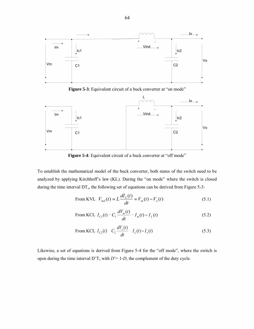
64
Vm
ImIc1
C1
+ -Vind
C2
Ic2
Io
Vo
Figure 5-3: Equivalent circuit of a buck converter at “on mode”
Vm
ImIc1
C1
+ -Vind
C2
Ic2
Io
Vo
L
Figure 5-4: Equivalent circuit of a buck converter at “off mode”
To establish the mathematical model of the buck converter, both states of the switch need to be
analyzed by applying Kirchhoff’s law (KL). During the “on mode” where the switch is closed
during the time interval DTs, the following set of equations can be derived from Figure 5-3:
From KVL )()()()( tVtVdt
tdILtV omL
ind (5.1)
From KCL )()()(
)( 11 tItIdt
tdVCtI Lm
mC (5.2)
From KCL )()()(
)( 22 tItIdt
tdVCtI oL
oC (5.3)
Likewise, a set of equations is derived from Figure 5-4 for the “off mode”, where the switch is
open during the time interval D’Ts with D’= 1-D, the complement of the duty cycle.
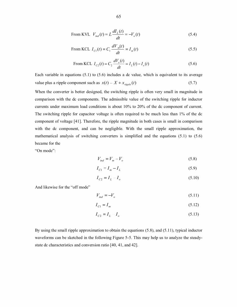
65
From KVL )()()( tVdt
tdILtV oL
ind (5.4)
From KCL )()(
)( 11 tIdt
tdVCtI m
mC (5.5)
From KCL )()()(
)( 22 tItIdt
tdVCtI oL
oC (5.6)
Each variable in equations (5.1) to (5.6) includes a dc value, which is equivalent to its average
value plus a ripple component such as )()( txXtx ripple (5.7)
When the converter is better designed, the switching ripple is often very small in magnitude in
comparison with the dc components. The admissible value of the switching ripple for inductor
currents under maximum load conditions is about 10% to 20% of the dc component of current.
The switching ripple for capacitor voltage is often required to be much less than 1% of the dc
component of voltage [41]. Therefore, the ripple magnitude in both cases is small in comparison
with the dc component, and can be negligible. With the small ripple approximation, the
mathematical analysis of switching converters is simplified and the equations (5.1) to (5.6)
became for the
“On mode”:
omind VVV (5.8)
LmC III 1 (5.9)
oLC III 2 (5.10)
And likewise for the “off mode”
oind VV (5.11)
mC II 1 (5.12)
oLC III 2 (5.13)
By using the small ripple approximation to obtain the equations (5.8), and (5.11), typical inductor
waveforms can be sketched in the following Figure 5-5. This may help us to analyze the steady-
state dc characteristics and conversion ratio [40, 41, and 42].
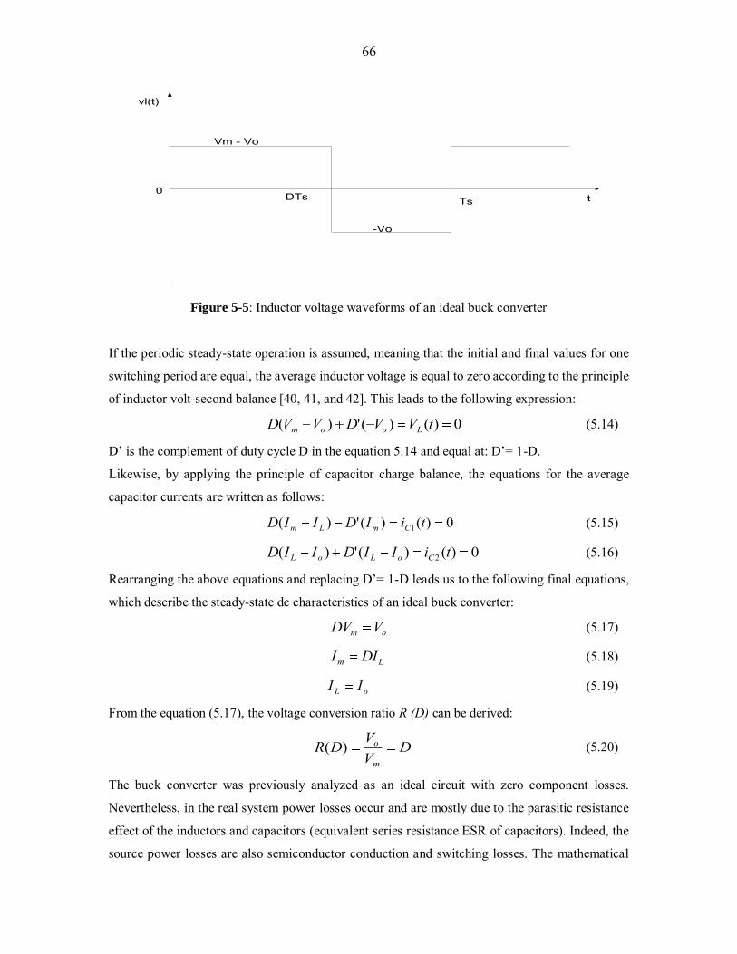
66
vl(t)
Vm - Vo
-Vo
DTs Ts0
t
Figure 5-5: Inductor voltage waveforms of an ideal buck converter
If the periodic steady-state operation is assumed, meaning that the initial and final values for one
switching period are equal, the average inductor voltage is equal to zero according to the principle
of inductor volt-second balance [40, 41, and 42]. This leads to the following expression:
0)()(')( tVVDVVD Loom (5.14)
D’ is the complement of duty cycle D in the equation 5.14 and equal at: D’= 1-D.
Likewise, by applying the principle of capacitor charge balance, the equations for the average
capacitor currents are written as follows:
0)()(')( 1 tiIDIID CmLm (5.15)
0)()(')( 2 tiIIDIID CoLoL (5.16)
Rearranging the above equations and replacing D’= 1-D leads us to the following final equations,
which describe the steady-state dc characteristics of an ideal buck converter:
om VDV (5.17)
Lm DII (5.18)
oL II (5.19)
From the equation (5.17), the voltage conversion ratio R (D) can be derived:
DVVDR
m
o)( (5.20)
The buck converter was previously analyzed as an ideal circuit with zero component losses.
Nevertheless, in the real system power losses occur and are mostly due to the parasitic resistance
effect of the inductors and capacitors (equivalent series resistance ESR of capacitors). Indeed, the
source power losses are also semiconductor conduction and switching losses. The mathematical
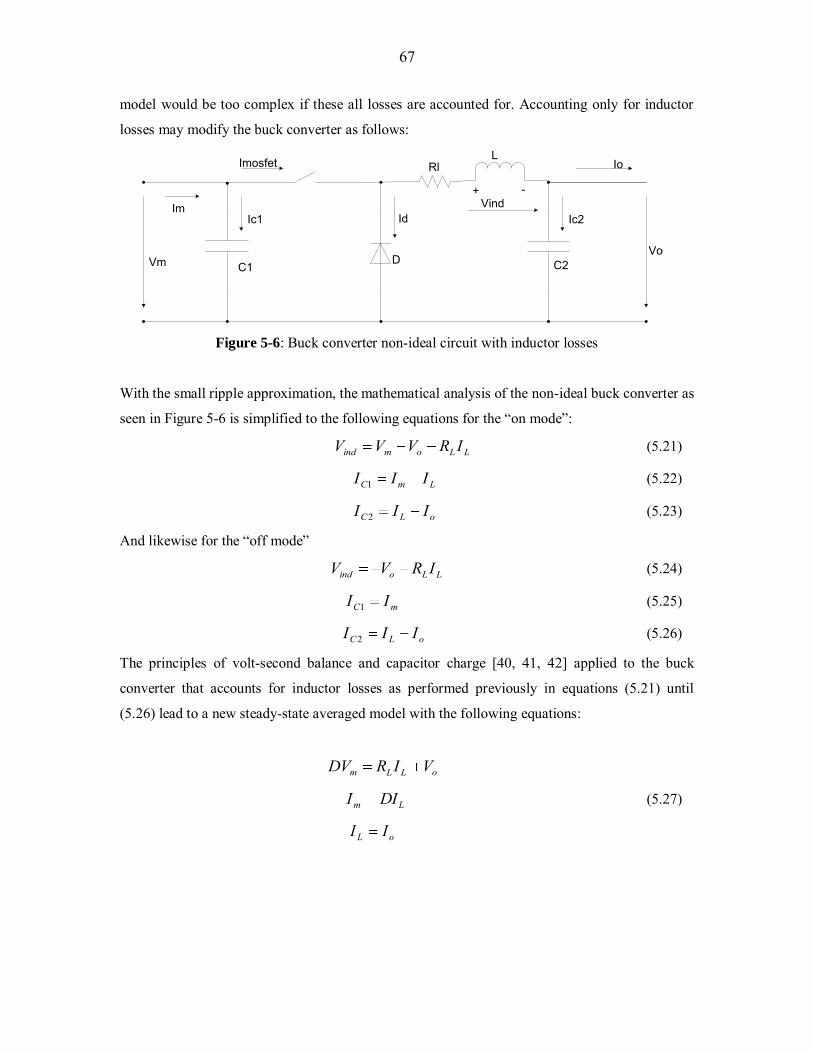
67
model would be too complex if these all losses are accounted for. Accounting only for inductor
losses may modify the buck converter as follows:
Vm
ImIc1
Imosfet
C1 D
IdVind
C2
Ic2
Io
Vo
+ -
LRl
Figure 5-6: Buck converter non-ideal circuit with inductor losses
With the small ripple approximation, the mathematical analysis of the non-ideal buck converter as
seen in Figure 5-6 is simplified to the following equations for the “on mode”:
LLomind IRVVV (5.21)
LmC III 1 (5.22)
oLC III 2 (5.23)
And likewise for the “off mode”
LLoind IRVV (5.24)
mC II 1 (5.25)
oLC III 2 (5.26)
The principles of volt-second balance and capacitor charge [40, 41, 42] applied to the buck
converter that accounts for inductor losses as performed previously in equations (5.21) until
(5.26) lead to a new steady-state averaged model with the following equations:
oLLm VIRDV
Lm DII (5.27)
oL II
68
5.2 .2 Dynamic analysis
A small-signal ac analysis is required to obtain the dynamic model of the buck converter.
To represent the converter’s steady-state dc behaviour, it has been shown previously that the ac
variations of a well-designed converter were neglected in the modelling operation. Let us now
investigate the ac small changes in the converter waveforms. The small ripple approximation
states that the converter waveforms are expressed as steady-state or quiescent values X plus small
ac variations )(ˆ tx : )(ˆ)( txXtx [39, 40, and 41].
Thus, all waveforms and signals of the converter can be now expressed as follows:
)(ˆ)( tvVtv mmm
)(ˆ)( tiIti mmm
)(ˆ)( 0 tvVtv oo
)(ˆ)( tiIti ooo (5.28)
)(ˆ)( tiIti LLL
)(ˆ)( tdDtd
Rearranging all the above equations into equations (5.14) to (5.16) leads to [43]:
dLLomL VtdtiRtvtvtddt
tdiL )(')()()()()( (5.29)
)()()()(
1 titdtidt
tdvC Lm
m (5.30)
)()()(2 titi
dttdvC oL
o (5.31)
The perturbation process where a small ac variation is added to the steady-state operating value
occurred by replacing the waveforms (5.28) into equations (5.29), (5.30), (5.31).
By arranging the set of these equations in such a way that the system can be linearized around the
quiescent operating point, and neglecting second-order perturbation terms, the final small-ac
model equations with only the first-order ac variations can be derived as follows [43]:
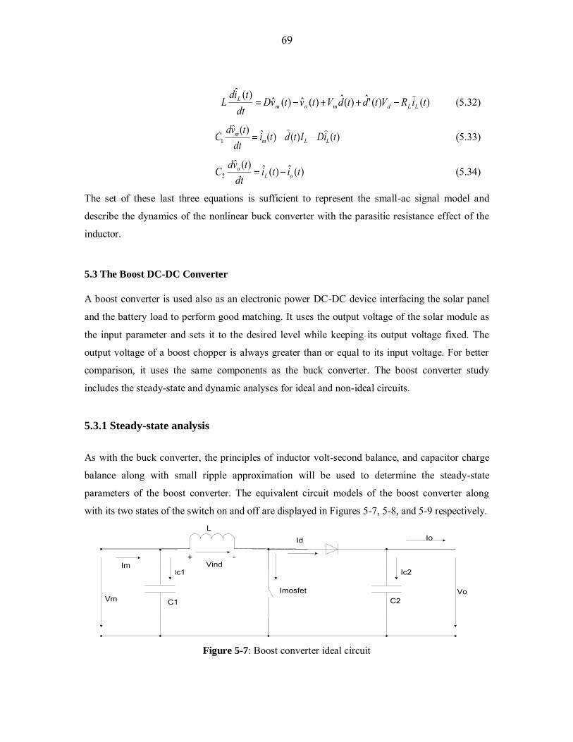
69
)()('ˆ)(ˆ)(ˆ)(ˆ)(ˆtiRVtdtdVtvtvD
dttid
L LLdmomL
(5.32)
)()()(ˆ)(ˆ1 tiDItdti
dttvdC LLm
m (5.33)
)(ˆ)(ˆ)(ˆ2 titi
dttvdC oL
o (5.34)
The set of these last three equations is sufficient to represent the small-ac signal model and
describe the dynamics of the nonlinear buck converter with the parasitic resistance effect of the
inductor.
5.3 The Boost DC-DC Converter
A boost converter is used also as an electronic power DC-DC device interfacing the solar panel
and the battery load to perform good matching. It uses the output voltage of the solar module as
the input parameter and sets it to the desired level while keeping its output voltage fixed. The
output voltage of a boost chopper is always greater than or equal to its input voltage. For better
comparison, it uses the same components as the buck converter. The boost converter study
includes the steady-state and dynamic analyses for ideal and non-ideal circuits.
5.3.1 Steady-state analysis
As with the buck converter, the principles of inductor volt-second balance, and capacitor charge
balance along with small ripple approximation will be used to determine the steady-state
parameters of the boost converter. The equivalent circuit models of the boost converter along
with its two states of the switch on and off are displayed in Figures 5-7, 5-8, and 5-9 respectively.
Vm
ImIc1
ImosfetC1
Id
Vind
C2
Ic2
Io
Vo
+ -
L
Figure 5-7: Boost converter ideal circuit
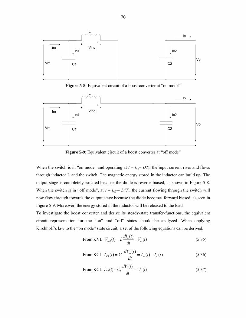
70
Vm
ImIc1
C1
Vind
C2
Ic2
Io
Vo
+ -
L
Figure 5-8: Equivalent circuit of a boost converter at “on mode”
Vm
ImIc1
C1
Vind
C2
Ic2
Io
Vo
+ -
L
Figure 5-9: Equivalent circuit of a boost converter at “off mode”
When the switch is in “on mode” and operating at t = ton= DTs, the input current rises and flows
through inductor L and the switch. The magnetic energy stored in the inductor can build up. The
output stage is completely isolated because the diode is reverse biased, as shown in Figure 5-8.
When the switch is in “off mode”, at t = toff = D’Ts, the current flowing through the switch will
now flow through towards the output stage because the diode becomes forward biased, as seen in
Figure 5-9. Moreover, the energy stored in the inductor will be released to the load.
To investigate the boost converter and derive its steady-state transfer-functions, the equivalent
circuit representation for the “on” and “off” states should be analyzed. When applying
Kirchhoff’s law to the “on mode” state circuit, a set of the following equations can be derived:
From KVL )()()( tVdt
tdILtV mL
ind (5.35)
From KCL )()()(
)( 11 tItIdt
tdVCtI Lm
mC (5.36)
From KCL )()()( 22 tIdt
tdVCtI oo
C (5.37)
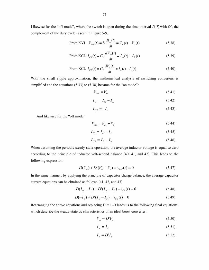
71
Likewise for the “off mode”, where the switch is open during the time interval D’Ts with D’, the
complement of the duty cycle is seen in Figure 5-9.
From KVL )()()(
)( tVtVdt
tdILtV om
Lind (5.38)
From KCL )()()(
)( 11 tItIdt
tdVCtI Lm
mC (5.39)
From KCL )()()(
)( 22 tItIdt
tdVCtI oL
oC (5.40)
With the small ripple approximation, the mathematical analysis of switching converters is
simplified and the equations (5.33) to (5.38) became for the “on mode”:
mind VV (5.41)
LmC III 1 (5.42)
oC II 2 (5.43)
And likewise for the “off mode”
omind VVV (5.44)
LmC III 1 (5.45)
oLC III 2 (5.46)
When assuming the periodic steady-state operation, the average inductor voltage is equal to zero
according to the principle of inductor volt-second balance [40, 41, and 42]. This leads to the
following expression:
0)()(')( tvVVDVD indomm (5.47)
In the same manner, by applying the principle of capacitor charge balance, the average capacitor
current equations can be obtained as follows [41, 42, and 43]:
0)()(')( 1 tiIIDIID CLmLm (5.48)
0)()(')( 2 tiIIDID CoLo (5.49)
Rearranging the above equations and replacing D’= 1-D leads us to the following final equations,
which describe the steady-state dc characteristics of an ideal boost converter:
om VDV ' (5.50)
Lm II (5.51)
Lo IDI ' (5.52)
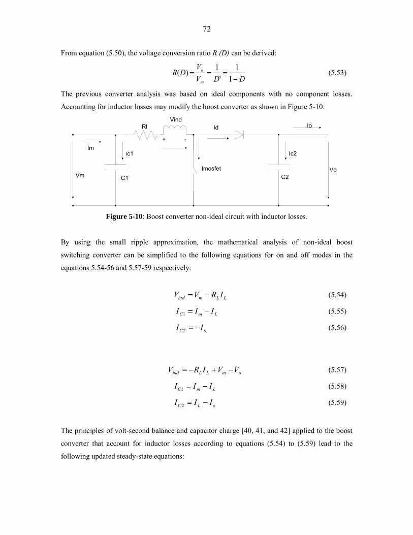
72
From equation (5.50), the voltage conversion ratio R (D) can be derived:
DDV
VDR
m
o
11
'1)( (5.53)
The previous converter analysis was based on ideal components with no component losses.
Accounting for inductor losses may modify the boost converter as shown in Figure 5-10:
Vm
ImIc1
ImosfetC1
IdVind
C2
Ic2
Io
Vo
+ -
Rl
Figure 5-10: Boost converter non-ideal circuit with inductor losses.
By using the small ripple approximation, the mathematical analysis of non-ideal boost
switching converter can be simplified to the following equations for on and off modes in the
equations 5.54-56 and 5.57-59 respectively:
LLmind IRVV (5.54)
LmC III 1 (5.55)
oC II 2 (5.56)
omLLind VVIRV (5.57)
LmC III 1 (5.58)
oLC III 2 (5.59)
The principles of volt-second balance and capacitor charge [40, 41, and 42] applied to the boost
converter that account for inductor losses according to equations (5.54) to (5.59) lead to the
following updated steady-state equations:
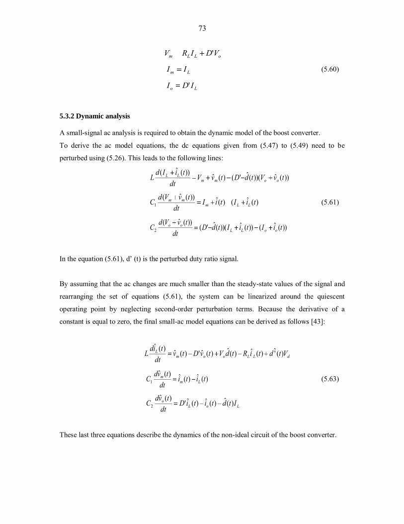
73
oLLm VDIRV '
Lm II (5.60)
Lo IDI '
5.3.2 Dynamic analysis
A small-signal ac analysis is required to obtain the dynamic model of the boost converter.
To derive the ac model equations, the dc equations given from (5.47) to (5.49) need to be
perturbed using (5.26). This leads to the following lines:
))(ˆ))((ˆ'()(ˆ))(ˆ( tvVtdDtvV
dttiIdL oomm
LL
)(ˆ()(ˆ))(ˆ(1 tiItiI
dttvVdC LLm
mm (5.61)
))(ˆ())(ˆ))((ˆ'())(ˆ(2 tiItiItdD
dttvVdC ooLL
oo
In the equation (5.61), d’ (t) is the perturbed duty ratio signal.
By assuming that the ac changes are much smaller than the steady-state values of the signal and
rearranging the set of equations (5.61), the system can be linearized around the quiescent
operating point by neglecting second-order perturbation terms. Because the derivative of a
constant is equal to zero, the final small-ac model equations can be derived as follows [43]:
dLLoomL VtdtiRtdVtvDtvdt
tidL )('̂)(ˆ)(ˆ)(ˆ')(ˆ)(ˆ
)(ˆ)(ˆ)(ˆ1 titi
dttvdC Lm
m (5.63)
LoLo ItdtitiDdt
tvdC )(ˆ)(ˆ)(ˆ')(ˆ2
These last three equations describe the dynamics of the non-ideal circuit of the boost converter.

74
5.4 Converter Topology Analysis and Comparison
This part of the chapter includes a comparative assessment between two converter topologies
interfacing the PV panel and the load battery and assists in choosing a suitable chopper for the
current stand-alone PV system. Two basic non-isolated boost and buck DC-DC choppers are
frequently used in PV power systems due to their advantages of simplicity and efficiency. The
two DC-DC converter topologies are compared on the basis of their dynamic models, frequency
characteristics, and component costs as they operate as the power interface between the PV panel
and a constant voltage battery load. Both DC-DC choppers are operating in Continuous
Conduction Mode (CCM) and are designed on the basis of the specifications provided in Table 5-
1 [44].
Table 5-1: Design specifications
Topology Buck converter Boost Converter
Nominal input voltage 17.3V 17.3V
Maximum input voltage 24V 24V
Nominal output voltage 12V 24V
Maximum output voltage 15V 30V
Nominal solar power 50W 50W
Maximum solar power 60W 60W
Switching frequency 40kHz 40kHz
Max inductor current ripple 10% 10%
Maximum input voltage ripple 0.5% 0.5%
Maximum output voltage ripple (%) 0.5% 0.5%
Convection Natural Natural
Efficiency > 90% > 90%
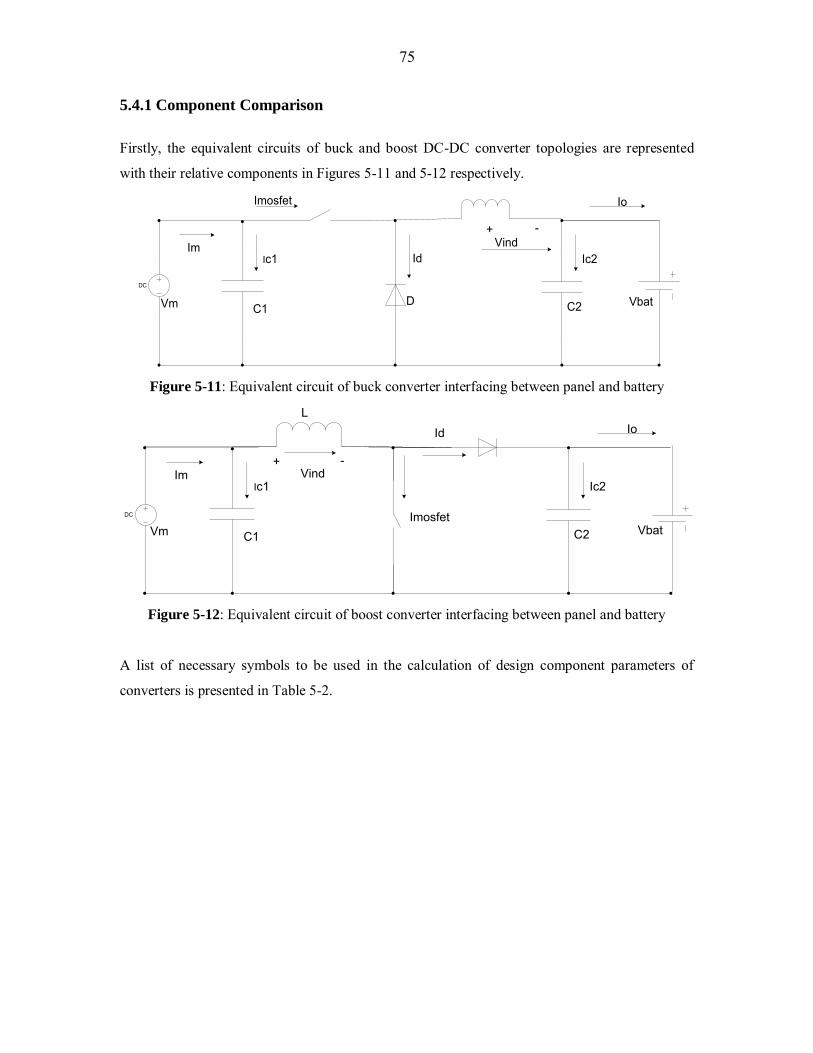
75
5.4.1 Component Comparison
Firstly, the equivalent circuits of buck and boost DC-DC converter topologies are represented
with their relative components in Figures 5-11 and 5-12 respectively.
Vm
ImIc1
Imosfet
C1 D
IdVind
C2
Ic2
Io
+ -
DC
Vbat
Figure 5-11: Equivalent circuit of buck converter interfacing between panel and battery
Vm
ImIc1
ImosfetC1
Id
Vind
C2
Ic2
Io
+ -
L
DC
Vbat
Figure 5-12: Equivalent circuit of boost converter interfacing between panel and battery
A list of necessary symbols to be used in the calculation of design component parameters of
converters is presented in Table 5-2.

76
Table 5-2: List of symbols
Symbols Designation
C1 Input capacitor
C2 Output capacitor
L Inductor
Vm Steady-state photovoltaic module or input voltage
∆vm Value of photovoltaic voltage ripple
Vbat Steady-state battery or output voltage
∆v Value of output voltage ripple
Im Steady-state photovoltaic module or input current
∆iL Value of inductor current ripple
Io Steady-state output current
D Duty cycle
fs Switching frequency
Both converters have different features. The boost chopper has a discontinuous output current and
a continuous input current. Conversely, the buck chopper has a discontinuous input current and a
continuous output current. In order to obtain the best comparison, the two choppers need to
follow the same design specifications with different output voltages as tabulated in Table 5-1.
The different inductance and capacitance design values and the RMS currents passing through all
components in the equivalent circuits can now be calculated for both converters using the basic
formulae on pages [44, 45]:

77
For the buck converter,
sm
m
fvDI
C2
)1(1
s
L
vfiC
82
sL
o
fiDV
L2
)1(
12
1.2
1rDDII oC (5.64)
122rII oC
)1( DII od
12
12rII oL
12
12rDII oMOSFET
o
L
Iir
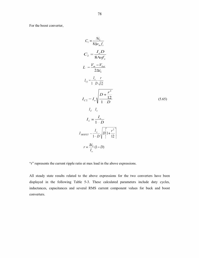
78
For the boost converter,
sm
L
fviC
81
s
o
vfDIC
82
L
batm
iVVL
2
1211r
DII o
C
D
rDII oC 1
12
2
2 (5.65)
od II
D
II oL 1
12
11
2rDD
II o
MOSFET
)1( DIiro
L
“r” represents the current ripple ratio at max load in the above expressions.
All steady state results related to the above expressions for the two converters have been
displayed in the following Table 5-3. These calculated parameters include duty cycles,
inductances, capacitances and several RMS current component values for buck and boost
converters.

79
Table 5-3: Calculated values based on design specifications of converters
Designation Buck Converter Boost Converter
L 137.8µH 236µH
C1 52µF 13.9µF
C2 21.69µF 22.92µF
IC1 1.42A 0.11A
IC2 0.12A 1.78A
Id 0.55A 2.08A
IL 4.16A 4A
ISW 3.88A 2.34A
R 0.1 0.11
Dmax 0.867 0.423
Io 4.166A 2.08A
Based on the above theoretical calculated values, it can be demonstrated that to achieve the same
ripple of inductor current r, the boost converter requires more inductance than the buck converter
while its RMS inductor current IL is less than that of the buck converter.
With regard to the input capacitors, the boost topology needs a small and cheap capacitor to
further smooth the PV current and voltage, which is already smooth, as its inductor current is
without any input capacitor. Conversely the buck topology requires a large and expensive
capacitor to smooth the discontinuous input current coming from the PV panel.
In the design process of the power switch Mosfet driver, the current rating in the buck converter
is higher than in the boost converter. This means that it will require a high-side Mosfet driver,
which is more complex and expensive than the one used in the boost converter.
Blocking diodes are usually used in PV installations to prevent reverse current from flowing back
from the battery into the PV cells during the night or during periods of low insolation. This avoids
leakage loss, extensive damage or even a fire. When selecting these diodes, the boost converter
presents some advantages over the buck one in that the freewheel diode in the boost chopper can
serve as the blocking diode to avoid the reverse current phenomena. This function is not possible
in the buck converter, requiring an additional component to use as blocking diode. This leads to
an increase in cost and additional power loss due to the forward voltage drop.
Indeed, the boost converter allows a continuous current to be drawn for the solar panel in both
switch situations. The boost converter therefore presents overall advantages over the buck

80
converter for the current specific PV application. This needs, however, to be confirmed at the
next stage related to the dynamic analysis.
5.4 .2 Modeling Comparison
In this section, buck and boost converters are compared on the basis of their dynamic models and
frequency characteristics. A dynamic model allows us to establish how changes in the duty cycle,
load current and input voltage affect the output voltage. The dynamic behavior of the converter is
hampered by the non-linear pulse-width modulation method and the time-varying nature of the
switching process. These converters are difficult to analyze directly using standard linear circuit
theory due to their inherently large signal. State-space averaging and small–signal modeling
techniques have traditionally been applied to overcome these difficulties. Moreover, linearizing
the converter circuit is crucial for understanding the converter circuit because it helps the designer
to apply the control theory.
The state-space averaged model generates the low-frequency small-signal ac equations of PWM
DC-DC converters and uses inductor current and capacitor voltage as two independent state
variables in the CCM.
The procedure for the state space averaged model can be described as follows [46, 47, and 48]:
First, draw the linear equivalent circuit for each state position of the switching converter.
Second, derive the circuit equations for each equivalent circuit using Kirchhoff’s voltage
and current laws.
Third, average each set of state-space equations and combine them into a single set by
summation, using the duty cycle as a weighting factor.
Fourth, perturb the averaged state equation to produce steady-state (DC) and dynamic
(AC) terms to eliminate non-linear cross product terms.
Fifth, transform the small signal AC equations into the complex frequency (S) domain to
solve for transfer function.
In the following analysis, parasitic effects have been taken into account for both inductor
converters as seen in Figures 5-6 and 5-10. Both converters operate in CCM. Indeed, the voltage
of battery in the current system is a constant DC bus due to the slow dynamics of the batteries and
the voltage change across the capacitor C2 can be ignored [43, 44]. The series resistance of the
inductor is selected from the datasheet [49]. The linearization of the system model using the set of
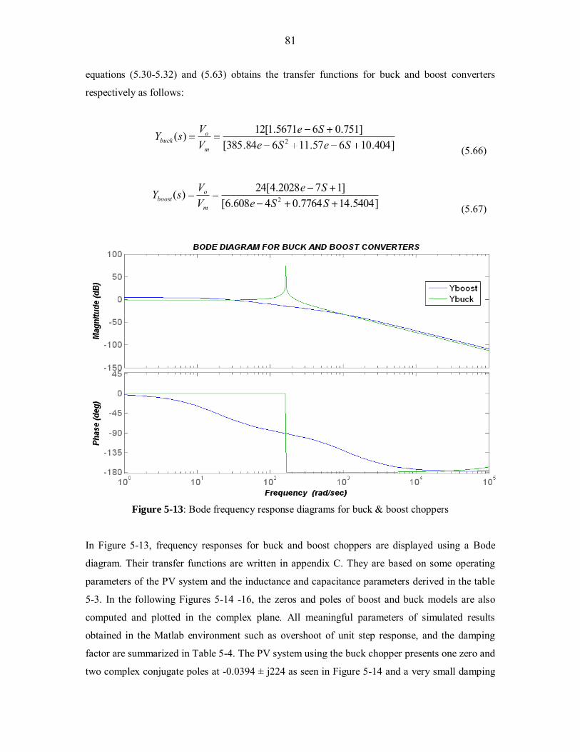
81
equations (5.30-5.32) and (5.63) obtains the transfer functions for buck and boost converters
respectively as follows:
]404.10657.11684.385[]751.065671.1[12)( 2 SeSe
SeVVsY
m
obuck
(5.66)
]5404.147764.04608.6[]172028.4[24)( 2 SSe
SeVVsY
m
oboost
(5.67)
Figure 5-13: Bode frequency response diagrams for buck & boost choppers
In Figure 5-13, frequency responses for buck and boost choppers are displayed using a Bode
diagram. Their transfer functions are written in appendix C. They are based on some operating
parameters of the PV system and the inductance and capacitance parameters derived in the table
5-3. In the following Figures 5-14 -16, the zeros and poles of boost and buck models are also
computed and plotted in the complex plane. All meaningful parameters of simulated results
obtained in the Matlab environment such as overshoot of unit step response, and the damping
factor are summarized in Table 5-4. The PV system using the buck chopper presents one zero and
two complex conjugate poles at -0.0394 ± j224 as seen in Figure 5-14 and a very small damping
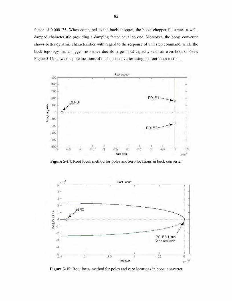
82
factor of 0.000175. When compared to the buck chopper, the boost chopper illustrates a well-
damped characteristic providing a damping factor equal to one. Moreover, the boost converter
shows better dynamic characteristics with regard to the response of unit step command, while the
buck topology has a bigger resonance due its large input capacity with an overshoot of 63%.
Figure 5-16 shows the pole locations of the boost converter using the root locus method.
Figure 5-14: Root locus method for poles and zero locations in buck converter
Figure 5-15: Root locus method for poles and zero locations in boost converter
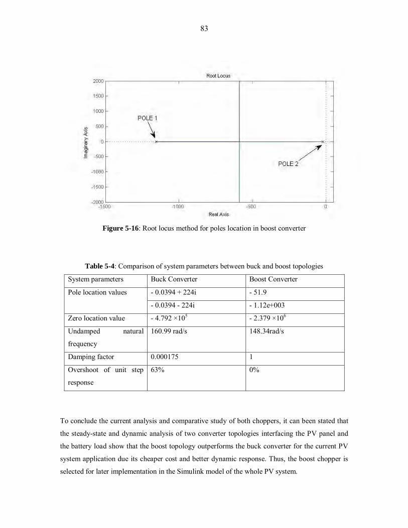
83
Figure 5-16: Root locus method for poles location in boost converter
Table 5-4: Comparison of system parameters between buck and boost topologies
System parameters Buck Converter Boost Converter
Pole location values - 0.0394 + 224i - 51.9
- 0.0394 - 224i - 1.12e+003
Zero location value - 4.792 ×10⁵ - 2.379 ×10⁶
Undamped natural
frequency
160.99 rad/s 148.34rad/s
Damping factor 0.000175 1
Overshoot of unit step
response
63% 0%
To conclude the current analysis and comparative study of both choppers, it can been stated that
the steady-state and dynamic analysis of two converter topologies interfacing the PV panel and
the battery load show that the boost topology outperforms the buck converter for the current PV
system application due its cheaper cost and better dynamic response. Thus, the boost chopper is
selected for later implementation in the Simulink model of the whole PV system.
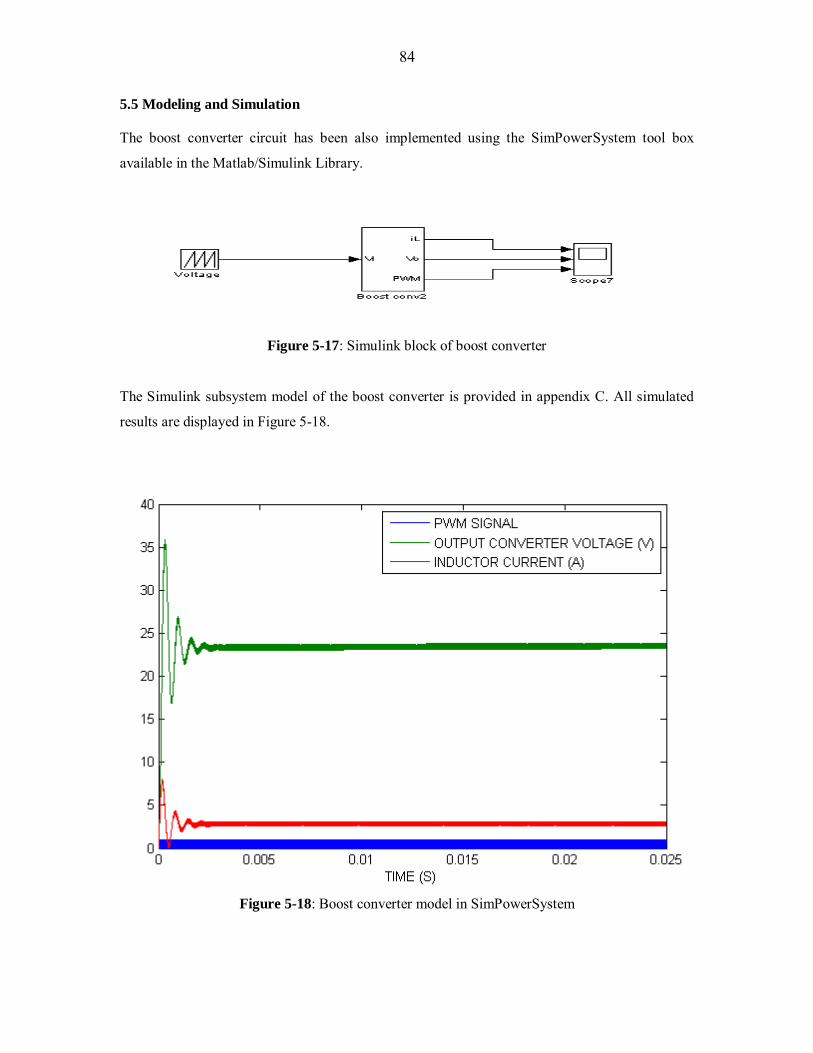
84
5.5 Modeling and Simulation
The boost converter circuit has been also implemented using the SimPowerSystem tool box
available in the Matlab/Simulink Library.
Figure 5-17: Simulink block of boost converter
The Simulink subsystem model of the boost converter is provided in appendix C. All simulated
results are displayed in Figure 5-18.
Figure 5-18: Boost converter model in SimPowerSystem
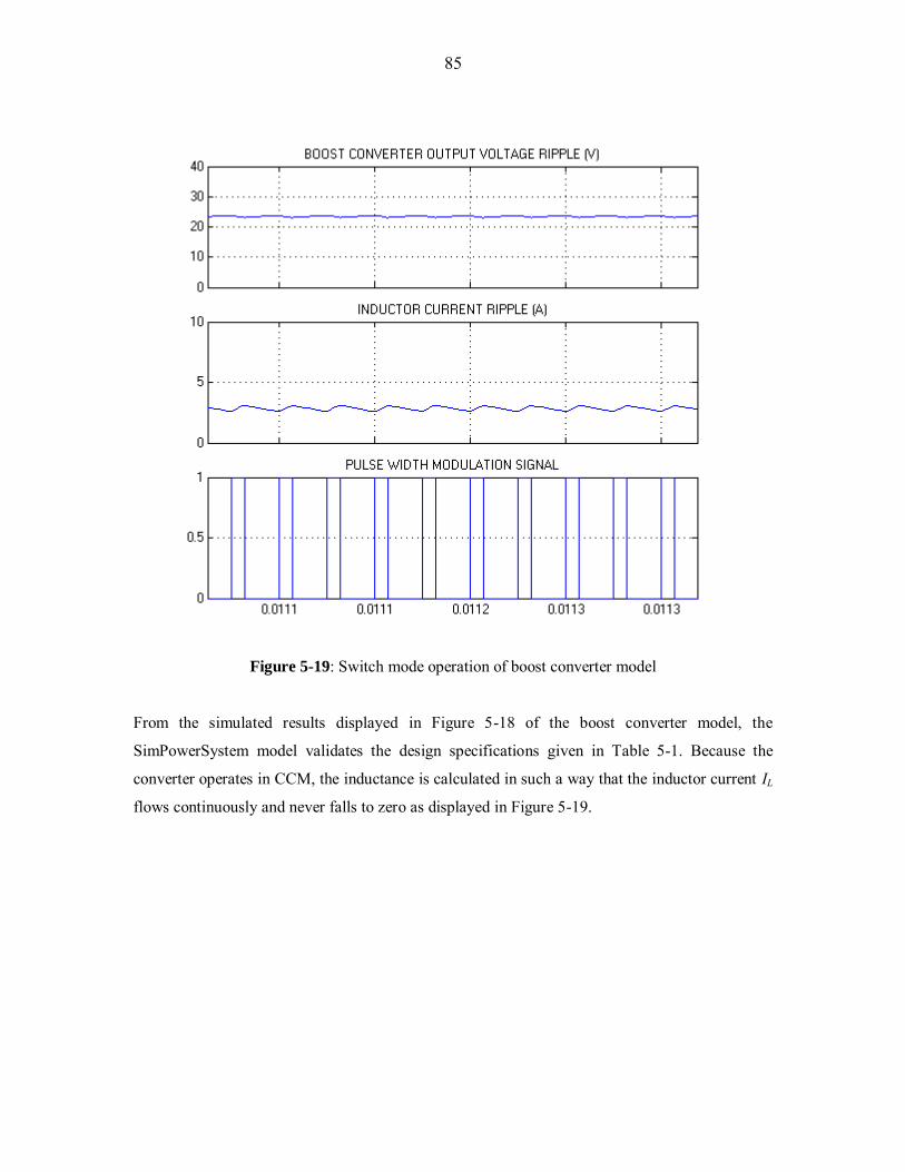
85
Figure 5-19: Switch mode operation of boost converter model
From the simulated results displayed in Figure 5-18 of the boost converter model, the
SimPowerSystem model validates the design specifications given in Table 5-1. Because the
converter operates in CCM, the inductance is calculated in such a way that the inductor current IL
flows continuously and never falls to zero as displayed in Figure 5-19.

86
Chapter 6: SYSTEM SIMULATION AND PERFORMANCE
ANALYSIS
6.1 Complete Simulink PV system
A PV solar panel, an MPPT algorithm, and a DC-DC boost converter have been modelled and
simulated separately in the previous chapters. They constitute the physical subsystems built for
the current PV power system. After being verified individually, they are connected together and
combined with the battery load in order to assess the overall PV system performance under
changing weather conditions. In chapter four dealing with the MPPT algorithm models, the two-
stage CV-IC algorithm was selected as the best MPPT algorithm when compared to the other four
algorithms, because it yields the highest tracking efficiencies under sunny and cloudy weather
conditions. Its superiority lies in its ability to use two different tracking approaches in different
operating weather conditions. Moreover, it provides the possibility of setting the perturbation step
size very small to improve accuracy without comprising dynamic performance. It can now be
implemented in the Simulink model of the complete PV system. Its performances need to be
investigated under slow and fast irradiance changes to further demonstrate its effectiveness when
compared to the standard conventional IC algorithm.
The solar panel and boost converter Simulink models have been set out in chapters three and five
respectively. The MPPT algorithm models were calculated via Matlab script codes in chapter
four. These codes are translated in the embedded Matlab function for IC and two-mode CV-IC
MPPT algorithms to obtain their Simulink models as shown in appendix D.
The following Figure 6-1 displays the boost converter with the pulse width modulation PWM
signal block. Its subsystem Simulink model can be found in appendix D.
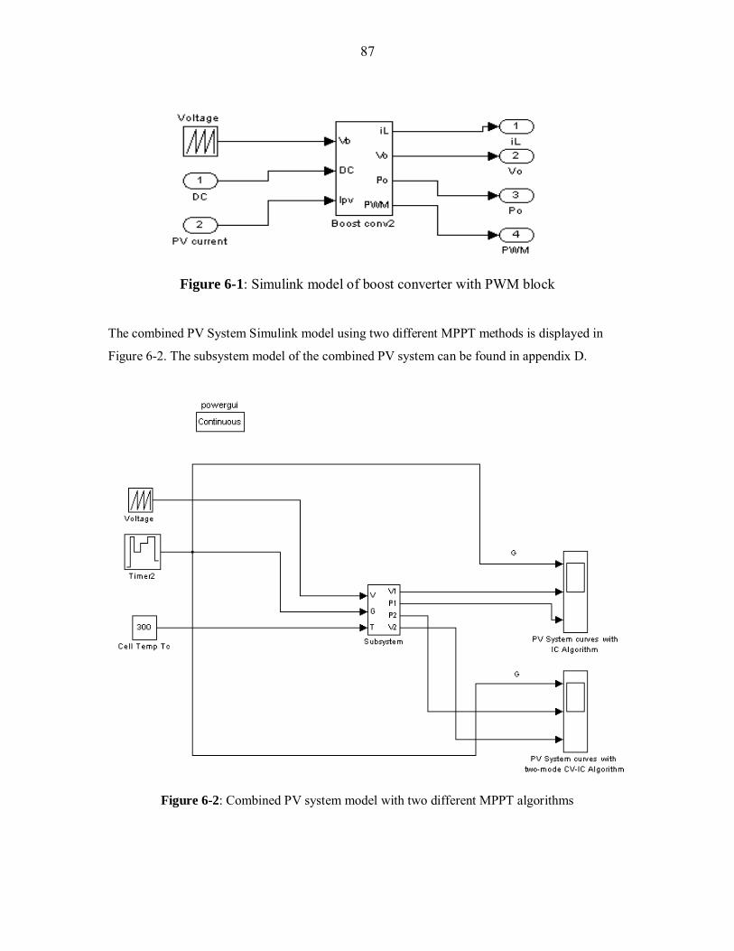
87
Figure 6-1: Simulink model of boost converter with PWM block
The combined PV System Simulink model using two different MPPT methods is displayed in
Figure 6-2. The subsystem model of the combined PV system can be found in appendix D.
Figure 6-2: Combined PV system model with two different MPPT algorithms
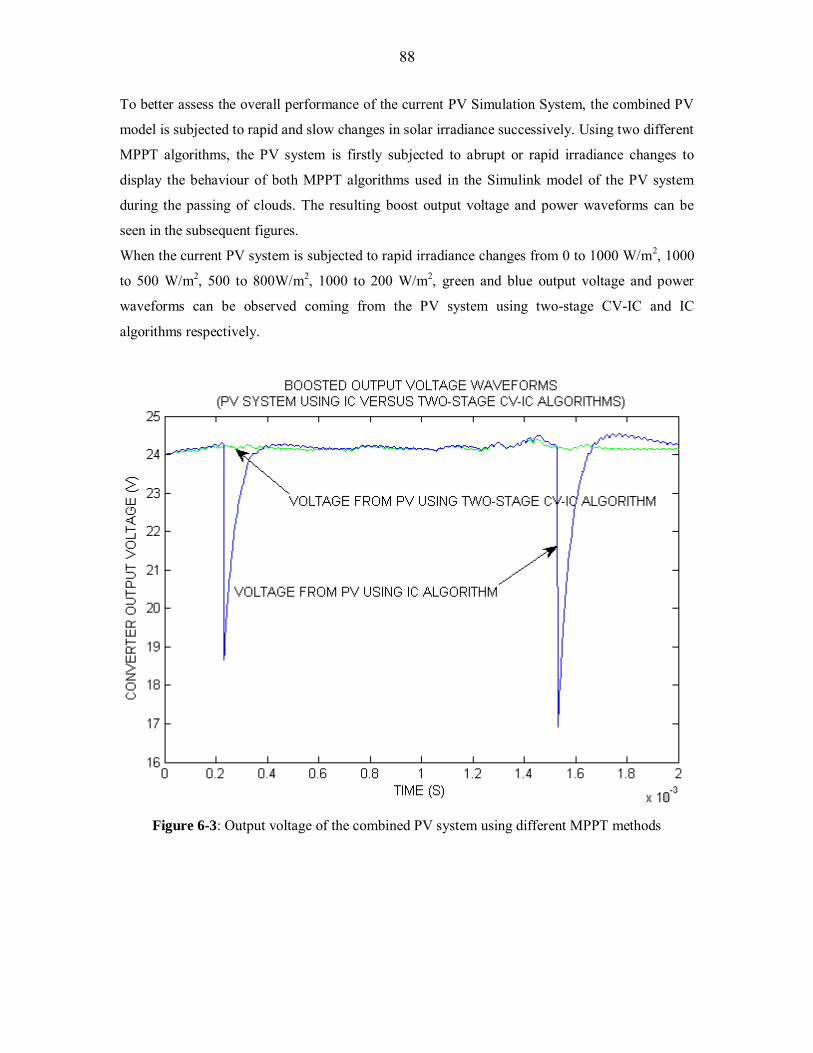
88
To better assess the overall performance of the current PV Simulation System, the combined PV
model is subjected to rapid and slow changes in solar irradiance successively. Using two different
MPPT algorithms, the PV system is firstly subjected to abrupt or rapid irradiance changes to
display the behaviour of both MPPT algorithms used in the Simulink model of the PV system
during the passing of clouds. The resulting boost output voltage and power waveforms can be
seen in the subsequent figures.
When the current PV system is subjected to rapid irradiance changes from 0 to 1000 W/m2, 1000
to 500 W/m2, 500 to 800W/m2, 1000 to 200 W/m2, green and blue output voltage and power
waveforms can be observed coming from the PV system using two-stage CV-IC and IC
algorithms respectively.
Figure 6-3: Output voltage of the combined PV system using different MPPT methods
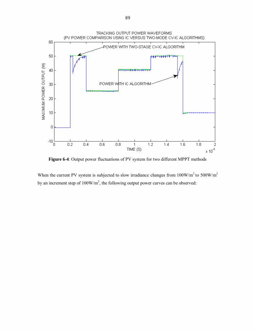
89
Figure 6-4: Output power fluctuations of PV system for two different MPPT methods
When the current PV system is subjected to slow irradiance changes from 100W/m2 to 500W/m2
by an increment step of 100W/m2, the following output power curves can be observed:
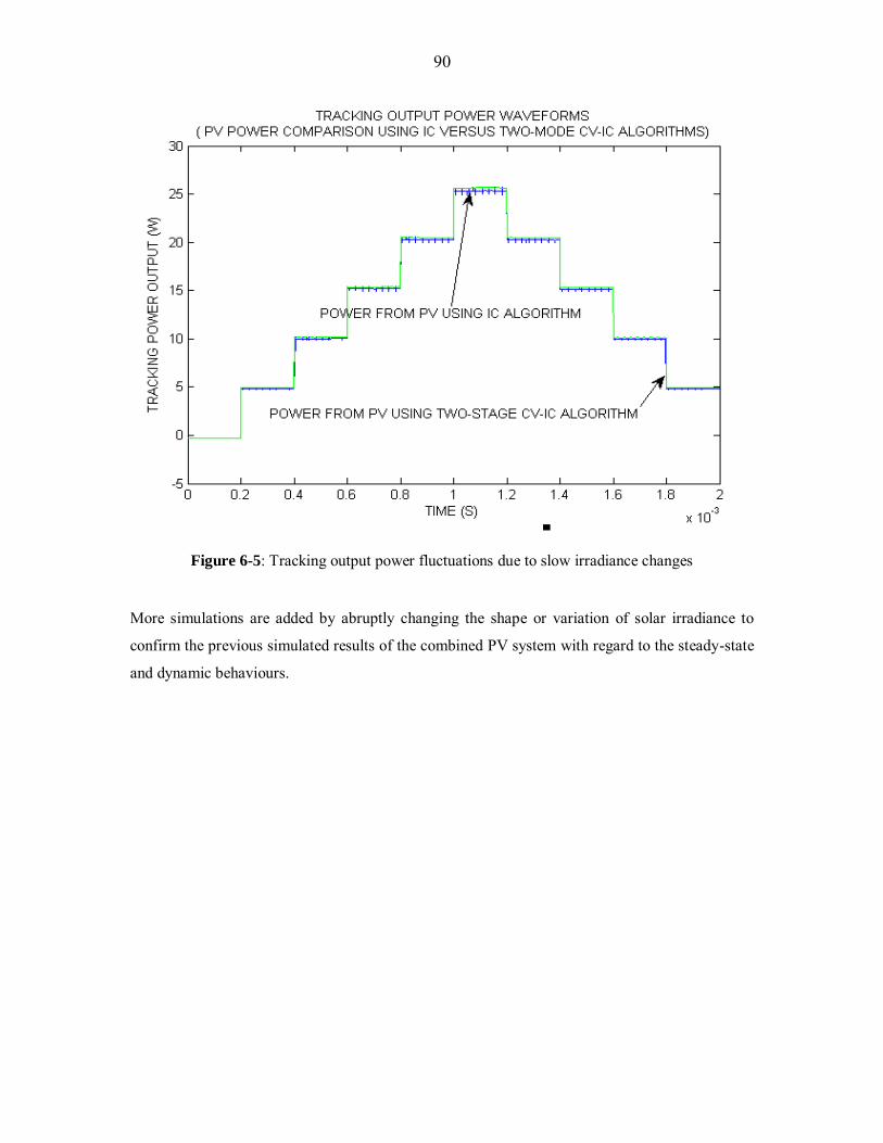
90
Figure 6-5: Tracking output power fluctuations due to slow irradiance changes
More simulations are added by abruptly changing the shape or variation of solar irradiance to
confirm the previous simulated results of the combined PV system with regard to the steady-state
and dynamic behaviours.
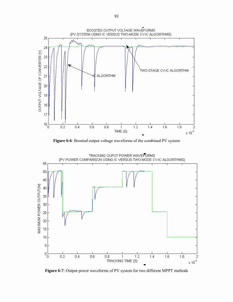
91
Figure 6-6: Boosted output voltage waveforms of the combined PV system
Figure 6-7: Output power waveforms of PV system for two different MPPT methods
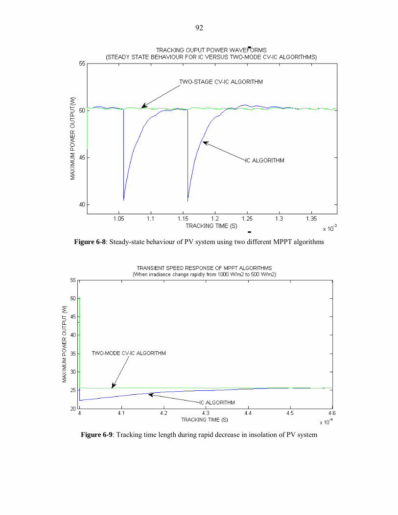
92
Figure 6-8: Steady-state behaviour of PV system using two different MPPT algorithms
Figure 6-9: Tracking time length during rapid decrease in insolation of PV system
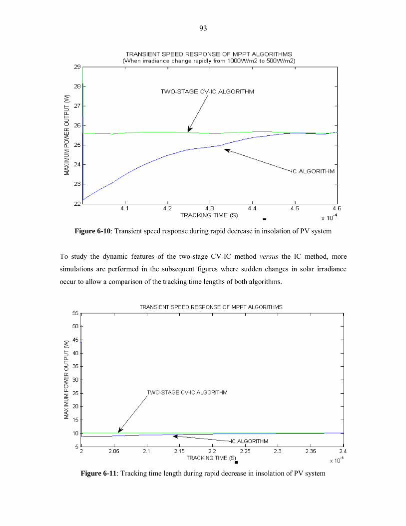
93
Figure 6-10: Transient speed response during rapid decrease in insolation of PV system
To study the dynamic features of the two-stage CV-IC method versus the IC method, more
simulations are performed in the subsequent figures where sudden changes in solar irradiance
occur to allow a comparison of the tracking time lengths of both algorithms.
Figure 6-11: Tracking time length during rapid decrease in insolation of PV system
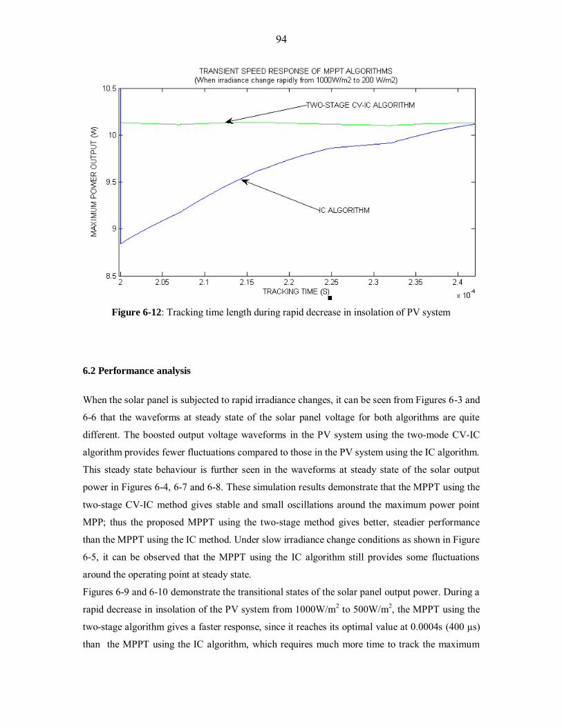
94
Figure 6-12: Tracking time length during rapid decrease in insolation of PV system
6.2 Performance analysis
When the solar panel is subjected to rapid irradiance changes, it can be seen from Figures 6-3 and
6-6 that the waveforms at steady state of the solar panel voltage for both algorithms are quite
different. The boosted output voltage waveforms in the PV system using the two-mode CV-IC
algorithm provides fewer fluctuations compared to those in the PV system using the IC algorithm.
This steady state behaviour is further seen in the waveforms at steady state of the solar output
power in Figures 6-4, 6-7 and 6-8. These simulation results demonstrate that the MPPT using the
two-stage CV-IC method gives stable and small oscillations around the maximum power point
MPP; thus the proposed MPPT using the two-stage method gives better, steadier performance
than the MPPT using the IC method. Under slow irradiance change conditions as shown in Figure
6-5, it can be observed that the MPPT using the IC algorithm still provides some fluctuations
around the operating point at steady state.
Figures 6-9 and 6-10 demonstrate the transitional states of the solar panel output power. During a
rapid decrease in insolation of the PV system from 1000W/m2 to 500W/m2, the MPPT using the
two-stage algorithm gives a faster response, since it reaches its optimal value at 0.0004s (400 µs)
than the MPPT using the IC algorithm, which requires much more time to track the maximum
95
power point (460 µs). Moreover, Figures 6-11 and 6-12 demonstrate the transient responses of
the tracked powers obtained from both MPPTs using IC versus CV-IC methods. It has been
observed that during a rapid decrease in insolation of the PV system from 1000W/m2 to
200W/m2, the time taken to track power using the IC method is approximately 0.000242s (242
µs) while the time achieved by the two-stage CV-IC method is 0.0002s (200µs). Therefore, the
MPPT using the two-stage algorithm reduces the convergence time taken to track the MPP and
improves the tracking speed response. It is quite efficient during the transitional state and
performs much better in cloudy weather scenario when compared to the standard IC method.
6.3 Conclusion
The simulated results of the combined Simulink PV model demonstrate that the PV system using
the two-stage CV-IC algorithm yields lower power fluctuations and shorter tracking times than
the PV system using the standard IC algorithm. The tracking speed of the MPPT using the two-
mode algorithm is 13% and 17.3% faster when subjected to a rapid decrease in insolation from
1000W/m2 to 500W/m2 and 1000W/m2 to 200W/m2 respectively as seen in Figures 6-10 and 6-12.
This means that the PV system using a two-stage CV-IC method loses less solar energy than the
standard IC method.
Furthermore, the simulated tracking output power waveforms displayed in Figures 6-4 and 6-8
show that the MPPT using a two-stage CV-IC method generates fewer oscillations around the
maximum power point MPP than the conventional IC method under rapid irradiance changes.
In conclusion, the simulated results of the PV system using a two-stage CV-IC algorithm show
good performances in both steady-state and transient operations. Hence, by implementing the
two-stage algorithm in the current PV system, the disadvantages of long tracking time and
increases in PV panel output power fluctuations when using the IC algorithm can be overcome.
96
Chapter 7: CONCLUSIONS AND FUTURE RESEARCH
7.1 Conclusions
This research study provides an efficient MPPT algorithm, called the two-stage CV-IC algorithm,
which combines the modified constant voltage CV and incremental conductance IC methods, and
can be applied in a photovoltaic home power supply.
It has been explained that when the solar PV panel is directly connected to the load, the power
delivered is not optimal. Moreover, solar PV power fluctuates due to variations in irradiance and
temperature levels. Thus, an MPPT system is needed to achieve the optimum or peak power
under changing environmental operating conditions. When a PV panel is equipped with an MPPT
system, it includes a solar panel, an MPPT algorithm, and a DC-DC converter.
Each component was modelled and simulated in a Matlab/Simulink environment; then all
subsystems were connected together and combined with the battery load to assess overall
performance under varying weather operating conditions.
A prototype 50W KYOCERA solar panel was evaluated using one diode Matlab and Simulink
models successively to test the influence of solar irradiation and temperatures. Both modeling
methods produced successful simulated results as expected and validated the electrical
characteristics provided in the datasheet of the manufacturer. The non-linearity behaviour of the
output characteristic of a PV panel was observed from the I-V and P-V curves, which are
dependent on insolation and cell temperature changes.
In this study, five MPPT algorithms, namely PO, IC, MPO, EPP and two-stage CV-IC methods
were investigated and analyzed through modelling and simulations. Firstly, the strengths and
weaknesses of classical MPPT methods were analyzed under a large range of operating
conditions. Subsequently, an optimized study solution of MPPT was performed to address the
drawbacks of the classical MPPT methods and few optimized MPPT solutions such as MPO,
EPP, and two-stage CV-IC algorithms were underlined. All five MPPT algorithms were written
in Matlab m-files, simulated, and compared in terms of their tracking performance. The improved
two-mode CV-IC algorithm performed better, especially under rapid changes in solar irradiance
(cloudy scenario) and yielded the highest tracking efficiencies of 99.77% and 99.92% under both
sunny and cloudy weather conditions respectively.
Thus, the two-stage MPPT method was selected to be implemented in the current Simulink PV
system simulation.
97
By using two tracking approaches to track the MPP in different situations, this improved two-
stage algorithm enabled both fast and fine tracking characteristics. A fast tracking approach was
achieved by the modified CV method when the variation in output current of PV panel is inferior
at 33% and a fine tracking approach was performed using the IC method, when the variation in
output current is superior at 33% (i.e. high insolation intensity). Furthermore, because the fast
and fine approaches are separately implemented in this improved method, the perturbation step
size can be set very small, which is different from the standard IC method where the width step
size should simultaneously meet the accuracy and tracking speed requirements. A few changes
were introduced in the improved two-mode algorithm by removing the expensive sensor device
used for the measurement of radiation. The converter duty cycle was used as a control variable,
simplifying the MPPT system in one direct control loop during its implementation in the whole
PV system Simulink model.
To further maximize the efficiency of PV system, a DC-DC buck and boost converter topology
and interface study between the PV panel and the battery load was performed in order to select
the appropriate chopper for the current PV system. In this comparative study based on the steady
state and dynamic analysis, the boost topology outperformed the buck converter due to its
cheaper implementation and better dynamic response and was also selected to be implemented in
the whole Simulink PV system simulation.
The simulated results of the combined Simulink PV system show that the PV system model using
the two-stage CV-IC algorithm generates better steady-state performances (lower power
fluctuations) and fast transient speed responses (shorter tracking times) than the PV using the
conventional original IC algorithm. The tracking speed of the MPPT using a two-mode algorithm
is 13% and 17.3% faster when subjected to a rapid decrease in insolation from 1000W/m2 to
500W/m2 and 1000W/m2 to 200W/m2 respectively. Thus, the PV system using the standard IC
method loses more power than the two-stage CV-IC method and is less efficient.
The simulated tracking output power waveforms show that the MPPT using the two-stage CV-IC
method gives stable and small oscillations around the maximum power point MPP than the
conventional IC method under abrupt irradiance changes. For a large solar PV array, these power
fluctuations are further reduced so that the output power and efficiency are significantly
improved, resulting in an increase in the total energy performance of the installation.
In conclusion, the PV system simulation using a two-mode CV-IC algorithm allows for a
reduction not only in the convergence time to track the MPP, but also in the fluctuations of power
98
at steady state. It therefore provides an overall better performance than the MPPT using the IC
method.
The two-stage CV-IC algorithm not only tracks the MPP more rapidly and constantly in order to
reduce the payback time, but it is able also to bypass multiple local maxima due to partial shading
effect, two important issues that occur in residential applications.
7.2 Future research
An experimental study of the current PV system needs to be undertaken in order to build a MPPT
system by physically implementing the two-stage algorithm in the microcontroller and charging
the lead-battery using the power delivered from the PV panel or array. Experimental results can
be deducted to validate the previous simulated results and would further assist in comparison to
the algorithm in reference [25].
Modern MPPT methods such Fuzzy Logic Controller (FLC) or artificial neural network control
could be used in the future simulation study especially when using a large solar array.
FLC offers the advantage of varying the increment of the duty cycle with accuracy and robustness
under changing environmental conditions. These intelligent algorithms are very promising
because they are adaptive, non-linear in nature and are convenient for PV control. FLC can be
further optimized by the use of genetic algorithms.
In the current study, the duty cycle is used as a control variable with the direct control MPPT
method but other advanced control methods can be implemented on FLC or Digital Signal
Processing (DSP) to further optimize the tracking process. Furthermore, when the output voltage
converter control is required, the design PI or PID compensators may be used for feedfoward and
feedback control loops. Their designs rely upon the transfer function derived from the state space
averaged small-signal ac model.
A theoretical assessment of interface and topology of the converter for the current PV system or
other PV configurations needs to be investigated with not only buck and boost converter
topologies but also other designed converters such as cuk or buck-boost converters along with
different load sizes and types.
In this study, the modelling of converters is based on the state space averaged method, which is
restricted to the small-signal, low-frequency domain and continuous conduction mode. The
dynamic analysis of converters could be performed using the discrete time domain method.
Future research could investigate some real-time identification methods to track the MPP rather
than tracking the MPP by the active operation of perturbation. Some learning-based MPPT

99
algorithms could also be used. Furthermore, more effective evaluation methods need be
developed to better compare different MPPT control algorithms.
Because the objective of the current study is to continually maximize the efficiency of the PV
system using an electronic tracking system MPPT, further research could focus on mechanical
tracking systems to study the placement of the panel or array along with its rotational adjustments
when weather conditions change in the specific area, which will further improve the efficiency of
the PV system.
A cost analysis of different MPPT techniques would further assist in comparing the tracking
methods as the high initial cost of the PV solar system is a major drawback in its rapid
deployment.
100
Bibliography
[1]. G.Boyle, “Renewable Energy, Power for a sustainable future”, Oxford University Press in
association with the Open University, second edition, 2004.
[2]. H. J. Moller, “Semiconductors for Solar Cells, Artech House”, Inc, Norwood, MA, 1993.
[3]. R.Faranda, S. Leva, “Energy comparison of MPPT techniques for PV Systems”, wseas
transactions on power systems. Issue 6, Volume 3, June 2008.
[4]. R.A.Cullen, “What is Maximum Power Point Tracking (MPPT) and How Does it Work?”
Blue Sky Energy, www.blueskyenergyinc.com, July 2000.
[5]. S.Bircan, “Battery Charger from Solar Cell”, Undergraduate thesis, The University of
Sydney, Faculty of Engineering, School of Electrical and Information Engineering, 2007.
[6]. P.Nattorn, “Analysis and Simulation tools for solar array power systems”, Doctoral thesis,
University of Central Florida, 2005.
[7]. J.M. Enrique, J.M. Andujar, M.A. Bohorquez, “A reliable, fast and low cost maximum power
point tracker for photovoltaic applications”, Science Direct, Solar Energy 84 (2010) 79-89, 14
November 2009.
[8]. D.P Hohm & M.E Ropp “Comparative Study of Maximum Power Point Tracking
Algorithms”, Progress in Photovoltaic: Research and Applications page 47-62, November 2002.
[9]. T.Tafticht, K.Agbossou and M.L Doumbia, “A new MPPT method for photovoltaic systems
used for hydrogen production”, COMPEL: The international Journal for Computation and
Mathematics in Electrical and Electronic Engineering. Vol. 26 No 1, pp 62-74, 2007.
[10]. V.Salas, E.Olias, A.Barrado, A.Lazaro, “Review of the Maximum Power Point Tracking
Algorithms for stand-alone photovoltaic systems”, Solar Energy Materials & Cells 90, 2006.
[11]. H.Yongji, and L.Deheng, “A new method for optimal output of a solar cell array”,
Proceedings of the IEE international Symposium on Industrial Electronics, pp 436-45, May 1992.
[12]. W.Xiao, “A modified adaptive hill climbing MPPT method for photovoltaic power
systems”, Master’s thesis, Shenyang Polytechnic University, 1991.
[13]. S.Balakrishna, Thansoe, A.Nabil, “The Study and Evaluation of Maximum Power Point
Tracking Systems”, International Conference on Energy and Environment, Malaysia, 2006.
[14]. J.Ahmad, and H.Kim, “A voltage based maximum power point tracker for Low
Power and Low Cost Photovoltaic Applications”, World Academy of Science, Engineering
And Technology 60, 2009.
101
[15]. T.Esram, and P. L.Chapman, “Comparison of Photovoltaic Array Maximum Power Point
Tracking Techniques”, IEE transactions on Energy conversion, Vol. 22, No 2, June 2007.
[16]. D.Sera, T.Kerekes, R.Teodorescu, and F.Blaabjerg, “Improved MPPT method for
rapidly changing environmental conditions”, IEEE ISIE 2006, Montreal, Quebec, Canada,
9-12 July, 2006.
[17]. S.Jain, and V.Agarwal, “A New Algorithm for Rapid Tracking of Approximate
Maximum Power Point in Photovoltaic Systems”, IEE Power Electronics letter, Vol. 2,
No 1, March 2004.
[18]. M.Milosevic, “On the Control of Distributed Generation in Power Systems”,
Doctoral Thesis, Swiss Federal Institute of Technology Zurich, 2007.
[19]. T.Tafticht, K.Agbossou, A.Cheriti and M.L Doumbia, “An Improved Maximum
Power Point Tracking Method for Photovoltaic Systems”, Renewable Energy 33 (2008)
1508-1516, 2008.
[20]. A. Yafaoui, B.Wu and R. Cheung, “Implementation of Maximum Power Point
Tracking Algorithm for Residential Photovoltaic Systems”, 2nd Canadian Solar Buildings
Conference Calgary, 10-14 June, 2007.
[21]. C.Shen, “Research and Improvement of Maximum Power Point Tracking for
Photovoltaic Systems”, PEDS2009, Taiwan, 2009.
[22]. X.Wang and A.P.Hu, “An Improved Maximum Power Point Tracking Algorithm for
Photovoltaic Systems”, Australasian Universities Power Engineering Conference, Brisbane,
Australia, 26-29 September, 2004.
[23]. J.H.Lee, H.Bae and B.H.Cho, “Advanced Incremental Conductance MPPT Algorithm with
a Variable Step Size”, Seoul National University, School of Electrical Engineering and Computer
Science, Seoul, Korea, 2006.
[24]. J.H.Lee, H. Bae, and B.H.Cho, “Constant Resistance Control of Solar Array Regulator
Using Average Current Mode Control”, Australasian Universities Power Engineering Conference
APEC06, 2006.
[25]. G.J. Yu, Y.S.Jung, J.Y.Choi, G.S. Kim, “A novel two-mode MPPT Control algorithm based
on comparative study of existing algorithms”, Solar Energy 76, 455-463, 2004.
[26]. W.Xiao, N.Ozog, and W.G.Dunford, “Topology Study of Photovoltaic Maximum Power
Point Tracking”, IEEE transactions on Industrial electronics, Vol. 54, No 3, June 2007.
[27]. A.J.Mahdi, W.H.Tang and Q.H.Wu, “Improvement of a MPPT Algorithm for PV systems
and its experimental validation”, ICREPQ’10, Granada (Spain), 25 March 2010.
102
[28]. Underwriters Laboratories, Inc., UL Standard 1703, “Flat-Plate Photovoltaic Modules and
Panels”, Northbrook, IL, 1993.
[29]. PV Glossary, Northern Arizona Wind & Sun, 2003
[30]. M.Francisco and G.Longatt, “Model of Photovoltaic Module in MatlabTM”, 2005.
[31]. G.Walker, “Evaluating MPPT Converter Topologies Using a Matlab PV Model”, Journal of
Electrical & Electronics Engineering, Australia, IEAust, Vol 21, No 1, pp 49-56, 2001.
[32]. H.L.Tsai, C. Tu, and Y. Su, “Development of Generalized Photovoltaic Model Using
Matlab/Simulink”, Proceedings of the World Congress on Engineering and Computer Science,
San Francisco, USA, 2008.
[33]. A.Oi, “Design and Simulation of Photovoltaic Water pumping System”, Master’s thesis,
California Polytechnic State University, September 2005.
[34]. M.A.Latif, A. Mohamed, “Maximum Photovoltaic Power Tracking Controller for Low
Power Applications”, 2nd WSEAS/IASME International Conference on Renewable Energy
Sources, Greece, October 26-28, 2008.
[35]. W.Shen, Y.Ding, F.H.Choo, “Mathematical model of a solar module for energy yield
simulation in photovoltaic systems”, PEDS, 2009.
[36]. J.H.Eckstein, “Detailed modelling of photovoltaic system components”, Master’s Thesis,
University of Wisconsin, Madison, 1990.
[37]. C.M.Bride, http://www.weathersa.co.za ([email protected]), “Hourly
Global Solar Radiation Data”, Upington, South African Weather Service, 1966.
[38]. G.M.S.Azevedo, M.C.Cavalcanti, and Z.D.Lins, “Comparative Evaluation of Maximum
Power Point Tracking Methods for Photovoltaic Systems”, Journal of Solar Energy Engineering,
Vol.131 /031006-1, August 2009. [39].T.P.Nguyen, “Solar Panel Maximum Power Point Tracker”, Undergraduate Thesis,
University of Queensland, 19 October 2001.
[40]. Mohan, Underland, Robbins. Power Electronics, Converters, Applications and Design,
Media Enhanced Third edition, John Wiley & Sons, 2003.
[41]. R.W. Erickson, “DC-DC Power Converters”, Article in Wiley Encyclopedia of Electrical
and Electronics Engineering, University of Colorado, 2000.
[42]. R.W.Erickson, D.Maksimovic, “Introduction to Power Electronics, Fundamentals of Power
Electronics” 2nd edition, Springer 2000, ECEN 2060, spring 2008.
[43]. W.Xiao, “Improved Control of Photovoltaic Interfaces”, Doctoral Thesis, British Columbia
University, April 2007.
103
[44]. W.Xiao, N.Ozog, and W.G.Dunford, “Topology Study of Photovoltaic Maximum Power
Point Tracking”, IEEE transactions on Industrial electronics, Vol. 54, No 3, June 2007.
[45].S.Maniktala, “Comparing Topologies and the (Design) Rules of the Game”,
http://www.national.com/nationaledge/mar03/article.html, Power Electronics Technology 2002
Proceedings for Power Systems World 2002 Conference, Rosemont, IL, November 2002.
[46]. R.P.Sevens and G.E.Bloom, “Modern DC-to-DC Switch Mode Power Converter Circuits”,
Van Nostrand Reinhold, New York 10003, 1985.
[47]. R. W. Erickson, “Fundamentals of Power Electronics’ slides”, Accompanying material for
Instructors, http://ece-www.colorado.edu/~pwrelect/book/slides/slidedir.html, 2002.
[48]. A.Ghosh and M.Kandpal, “State-space average modelling of DC-DC converters with
parasitic in Discontinuous Conduction Mode”, Undergraduate thesis, 2010.
[49]. W. C. So, C. K. Tse and Y. S. Lee, “Development of a Fuzzy Logic Controller for
DC/DC Converters: Design, Computer Simulation, and Experimental Evaluation”, IEEE
Transaction on Power Electronics, Vol. 11, pp. 24-32, January 1996.

APPENDIX A MATLAB Code for calculating the output current function Im
% modelling of KYOCERA SOLAR PANEL using the function KYOCERASOLAR_v50P
%
% the parameters are Vm (output module voltage), G (irradiation 1G=1kW/m^2)
% and T (Cell temperature C)
% the output is the module current Im
% Created by Cedrick, February, 2011
%**************************************************************************
Function Im = KYOCERASOLAR_v50P (Vm, G, T)
%//////////////////////////////////////////////////////////////////////////
%Electrical performance data for high efficiency multicrystal
%Photovoltaic module KD50SE- 1P model KYOCERASOLAR
T_Ref = 298; % Standard Kelvin temperature
Cn = 36; % Cell series number of solar KD50SE- 1P model KYOCERASOLAR panel
alpha = 1.84e-3; % Short circuit current coefficient of temperature
V_TRef = 22.1 /Cn; % Standard open circuit voltage taken from datasheet
I_TRef = 3.07; % Standard short circuit current taken from datasheet
%**************************************************************************
% Physical constants to be defined
k = 1.381e-23; % Stefan Boltzmann's constant (J/K)
q = 1.602e-19; % Charge of an electron (1 eV = 1.602e-19 J)
% Other Constants
A = 1.0; % Ideal diode quality factor depending on PV technology
En_band = 1.12; % Energy for band gap voltage, for polycrystalline-Si
TK = 273 + T; % Kelvin panel temperature
V_cell = Vm / Cn; % Voltage/cell
I_TK = I_TRef * (1 + (alpha * (TK - T_Ref))); % Short circuit current at TK
I_L = I_TK * G; % light photo current at G
%**************************************************************************
V_th = (k * A * T_Ref) / q; % Thermal voltage at T_Ref
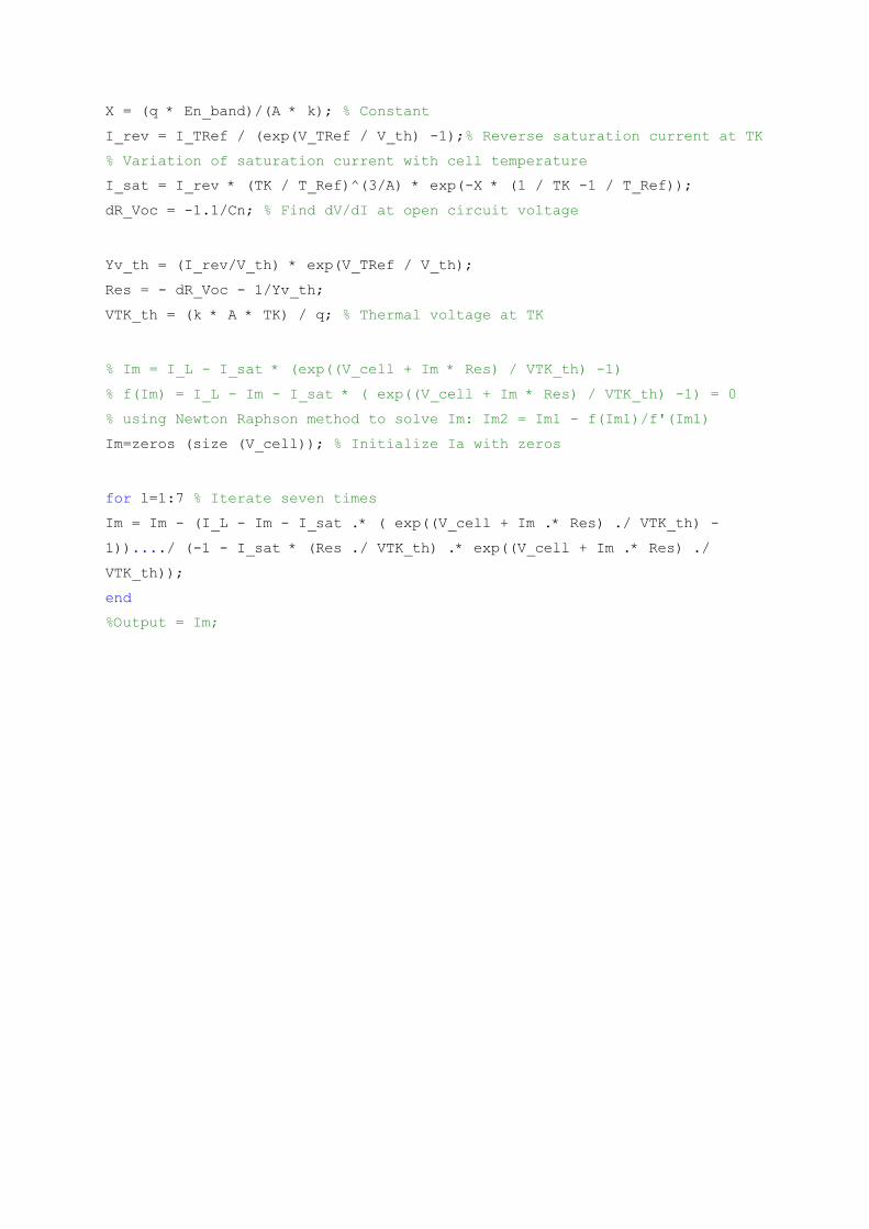
X = (q * En_band)/(A * k); % Constant
I_rev = I_TRef / (exp(V_TRef / V_th) -1);% Reverse saturation current at TK
% Variation of saturation current with cell temperature
I_sat = I_rev * (TK / T_Ref)^(3/A) * exp(-X * (1 / TK -1 / T_Ref));
dR_Voc = -1.1/Cn; % Find dV/dI at open circuit voltage
Yv_th = (I_rev/V_th) * exp(V_TRef / V_th);
Res = - dR_Voc - 1/Yv_th;
VTK_th = (k * A * TK) / q; % Thermal voltage at TK
% Im = I_L - I_sat * (exp((V_cell + Im * Res) / VTK_th) -1)
% f(Im) = I_L - Im - I_sat * ( exp((V_cell + Im * Res) / VTK_th) -1) = 0
% using Newton Raphson method to solve Im: Im2 = Im1 - f(Im1)/f'(Im1)
Im=zeros (size (V_cell)); % Initialize Ia with zeros
for l=1:7 % Iterate seven times
Im = Im - (I_L - Im - I_sat .* ( exp((V_cell + Im .* Res) ./ VTK_th) -
1))..../ (-1 - I_sat * (Res ./ VTK_th) .* exp((V_cell + Im .* Res) ./
VTK_th));
end
%Output = Im;

MATLAB M-files Code for plotting current-voltage and power- voltage curves under
change of solar irradiances and cell temperatures
% Script file to plot power-voltage curves of PV module for different
% solar irradiances (0.25, 0.50, 0.75, 1)
% Created by Cedrick, February, 2011
%///////////////////////////////////////////////////////////////
Clear;
Global T% makes variable T accessible on a global scope
T = 20; % Cell temperature
% Plot graph of Power vs. Voltage
figure
hold on
for G=0:0.25:1 % solar irradiance G (1 kW/m^2 = 1000 W/m^2)
% linspace creates a vector from 0 to 300 in increments of (100-T/15)
Vm = linspace (0, 100-T/15, 300);
Im = KYOCERASOLAR_v50P (Vm, G, T);
Power = Vm.*Im;
Plot (Vm, Power)
end
Title ('KYOCERASOLAR__50P P-V Curve')
Xlabel ('Panel Voltage (V)')
Ylabel('Panel Power (w)')
axis([0 25 0 55])
gtext('0.25')
gtext('0.5')
gtext('0.75')
gtext('1')
GRID ON
hold off
% Script file to plot power-voltage curves of PV module for different
% cell temperatures (20C, 40C, 60C, 80C)
% Created by Cedrick, February, 2011
%///////////////////////////////////////////////////////////////
Clear
Global T% makes variable T accessible on a global scope
G = 1; % solar irradiance G (1 kW/m^2 = 1000 W/m^2)
% Plot graph of Power vs. Voltage
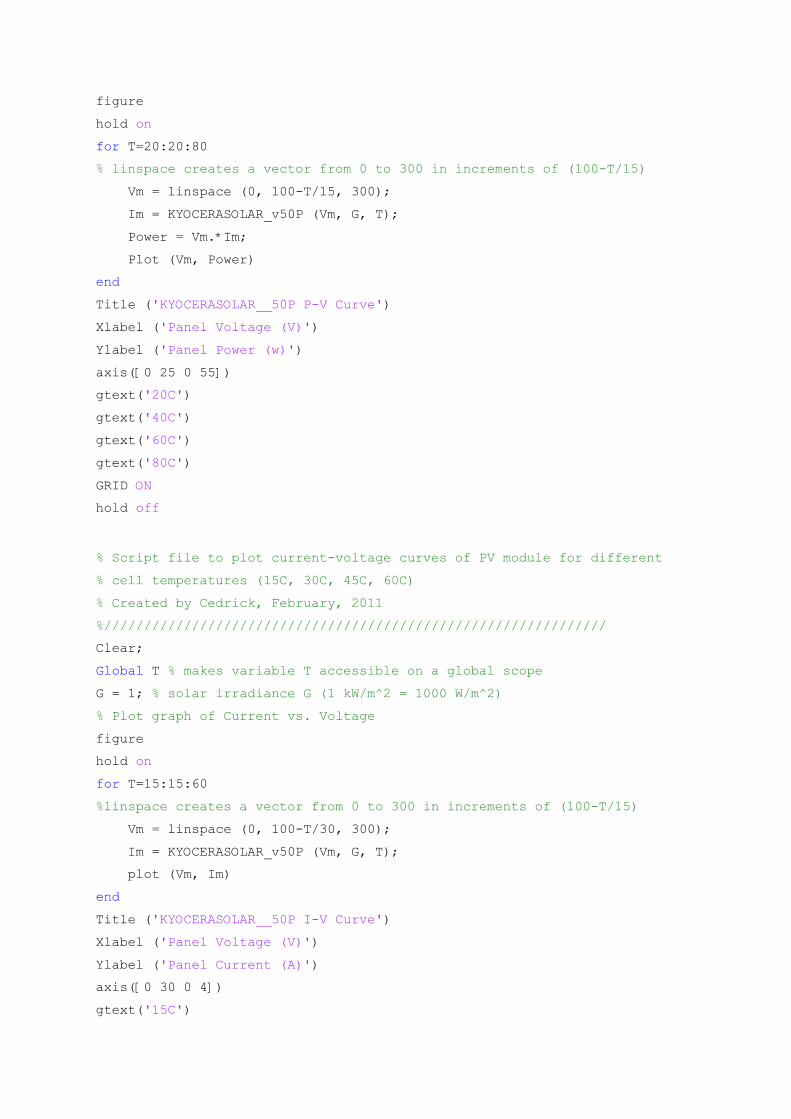
figure
hold on
for T=20:20:80
% linspace creates a vector from 0 to 300 in increments of (100-T/15)
Vm = linspace (0, 100-T/15, 300);
Im = KYOCERASOLAR_v50P (Vm, G, T);
Power = Vm.*Im;
Plot (Vm, Power)
end
Title ('KYOCERASOLAR__50P P-V Curve')
Xlabel ('Panel Voltage (V)')
Ylabel ('Panel Power (w)')
axis([0 25 0 55])
gtext('20C')
gtext('40C')
gtext('60C')
gtext('80C')
GRID ON
hold off
% Script file to plot current-voltage curves of PV module for different
% cell temperatures (15C, 30C, 45C, 60C)
% Created by Cedrick, February, 2011
%///////////////////////////////////////////////////////////////
Clear;
Global T % makes variable T accessible on a global scope
G = 1; % solar irradiance G (1 kW/m^2 = 1000 W/m^2)
% Plot graph of Current vs. Voltage
figure
hold on
for T=15:15:60
%linspace creates a vector from 0 to 300 in increments of (100-T/15)
Vm = linspace (0, 100-T/30, 300);
Im = KYOCERASOLAR_v50P (Vm, G, T);
plot (Vm, Im)
end
Title ('KYOCERASOLAR__50P I-V Curve')
Xlabel ('Panel Voltage (V)')
Ylabel ('Panel Current (A)')
axis([0 30 0 4])
gtext('15C')

gtext('30C')
gtext('45C')
gtext('60C')
grid on
hold off
% Script file to plot current-voltage curves of PV module for different
% solar irradiances (0.2, 0.40, 0.60, 0.80, 1)
% Created by Cedrick, February, 2011
%///////////////////////////////////////////////////////////////
Clear;
Global T% makes variable T accessible on a global scope
T = 20; % Cell temperature
% Plot graph of Current vs Voltage
figure
hold on
for G=0:0.2:1
%linspace creates a vector from 0 to 300 in increments of (100-T/15)
Vm = linspace (0, 100-T/15, 300);
Im = KYOCERASOLAR_v50P (Vm, G, T);
plot(Vm, Im)
end
title('KYOCERASOLAR__50P I-V Curve')
xlabel('Panel Voltage (V)')
ylabel('Panel Current (A)')
axis([0 30 0 4])
gtext('0.20')
gtext('0.40')
gtext('0.60')
gtext('0.80')
gtext('1')
grid on
hold off
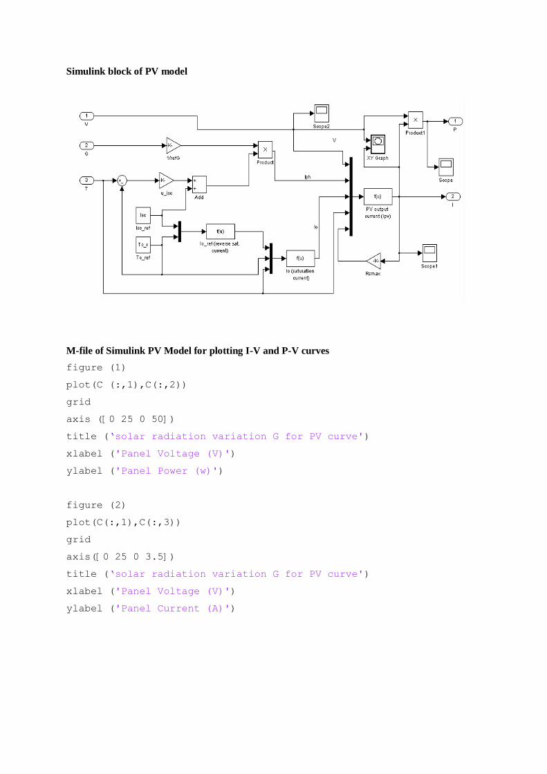
Simulink block of PV model
M-file of Simulink PV Model for plotting I-V and P-V curves
figure (1)
plot(C (:,1),C(:,2))
grid
axis ([0 25 0 50])
title (‘solar radiation variation G for PV curve')
xlabel ('Panel Voltage (V)')
ylabel ('Panel Power (w)')
figure (2)
plot(C(:,1),C(:,3))
grid
axis([0 25 0 3.5])
title (‘solar radiation variation G for PV curve')
xlabel ('Panel Voltage (V)')
ylabel ('Panel Current (A)')
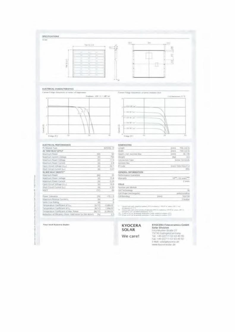
I
l I I
J l J 1 I
l I
' 1
... .... . .. '" - .. ..
" .. ~ ~
r + • ~~~
;:
··-f~ !\41Lf#•l• .
•
'
'
.._ ......... ,. __ .,._.
Qle!r'C~........,.fl ! 'ltoln (_r.JIII. eo.-. ,. - .. ... j.NOC!'!'= ----~ ~....,,_
Cf!'.!.IICWI\'oltg>~ i Sl'o't t""...n.r c.,.,.....,...;
""'"' ---·
..
...._.._..(..-~ .. \lfle~~ T ........ ~lll'!r:: ,...._._~,..
\((~
\\ \
~~-tll,a .......
1\ \
ttr.IUI.I If'
..., .. M ,.,., ~- ... "' " ... "' fill:' a ·~.!~~
M !:: loS .ISO oq ";'
"' ... , ,., .... • ... • .,.. .10 ..
>'"9 ·-~ ......, -1'~···
~f/11"-:"--.'-IIIXI:I*"""'•XIO•"""" N u
,_ . ...,. ____ . _ _... ....
!
......... .,.,. ........ -iilf'tiJ;,-.; _._. ...
"':'1" --,...,_.._ . -w.u ~!!!"~ , ... ,...........,. C,.""!-'~'
KYOCERA SOLAR
We care!
,..~.,._... '
..
...... ~Qr,•"C25.t
M ,_r!..t7ef ..... .. «> ,..., ., --
.. ...... ·-
KYOCOA ,IM<..,-.mlo GlnbH SolatO.-.bl~
f •l/ u. 1·Str-att' 21 .tl • Mi'~'l'loW7\.
TC'I· •ofl) tt•! n \-9J 93 4?9':. J,u: •4'1{017l1"i)9l,f?SQ (~~~·Ole' W'IWII - I'IX('f#J/ti.M.

APPENDIX B
MATLAB Code for calculating the theoretical maximum power (MPP) function
according to given irradiance and temperatures.
% Matlab function to calculate the theoretical maximum power point of
% KYOCERASOLAR_v50P when subjected to the variation of temperature and
% light levels
Function [Pm_th, Im_th, Vm_th] = det_max_KYOCERASOLAR_v50P (G, T)
% det_max: function to determine a theoretical maximum power point of
% solar panel
% [Pm_th, Im_th, Vm_th] = det_max (G, T)
% The parameters are G( solar irradiance) and T(Cell temperature)
% The outputs are Pm_th, Im_th, Vm_th
% Created by Cedrick, February, 2011
%////////////////////////////////////////////////////////////////
% Set initial conditions for Vm and Pm_th
Vm = 10;
Pm_th = 0;
% Find maximum power point
while Vm < 24-T/4
Im = KYOCERASOLAR_v50P (Vm, G, T);
Pm_new = Im * Vm;
if Pm_new > Pm_th
Pm_th = Pm_new;
Im_th = Im;
Vm_th = Vm;
end
Vm = Vm + .003;
end

MATLAB m-files script Code for calculating the maximum operating power of PO
algorithm under atmospheric sunny conditions
% MATLAB Script file for investigating the PO MPPT Algorithm under
% sunny weather conditions (slowly of solar irradiance G)
% Created by Cedrick, February, 2011
%%%%%%%%%%%%%%%%%%%%%%%%%%%%%%%%%%%%%%%%%%%%%%%%%%%%%%%%%%%%%%
Clear
Global T% makes variable T accessible on a global scope
% Initial Conditions
T = 25; % Temperature of the solar panel cell (C)
C = 0.1; % increment voltage (V)
G = 0.025; % solar irradiance
Vm = 17.3; % panel voltage (V)
Im = KYOCERASOLAR_v50P (Vm, G, T); % PV current of module
Pm = Vm * Im; % Panel power output
Vp_new = Vm + C; % updated reference panel voltage
% Create vectors for voltage and power data
Vm_arr = [];
Pm_arr = [];
Pmax_arr = [];
% Provide solar irradiation data for a sunny day at Upington
% Data stored in a 14 by 2 matrix, with column 1 being the time data and
% column 2 the irradiation data
G_data = [1 0.02; 2 0.204; 3 0.439; 4 0.664; 5 0.827; 6 0.981; 7 1.073; ...
8 1.073; 9 1; 10 0.868; 11 0.684; 12 0.449; 13 0.214; 14 0.03];
x_t = G_data(:,1)'; % Store time data in vector x_t (hour)
y_G = G_data(:,2)'; % Store irradiation data in vector y_G (Kw/m2)
x_ti = 1: 300; % Creates a 1 by 300 vector for interpolation
y_Gi = interp1 (x_t, y_G, x_ti,'linear'); % Perform linear interpolation
for i = 1:14
G = y_Gi (i); % Store interpolated values
new_Vm = Vp_new; % measure voltage
new_Im = KYOCERASOLAR_v50P (Vp_new, G, T); % measure current
Pm_new = new_Vm * new_Im; % Determine new Power
deltaPm = Pm_new - Pm; % Find the difference in power
% Start PO MPPT Algorithm
if deltaPm > 0
if new_Vm > Vm
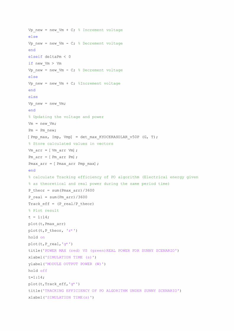
Vp_new = new_Vm + C; % Increment voltage
else
Vp_new = new_Vm - C; % Decrement voltage
end
elseif deltaPm < 0
if new_Vm > Vm
Vp_new = new_Vm - C; % Decrement voltage
else
Vp_new = new_Vm + C; %Increment voltage
end
else
Vp_new = new_Vm;
end
% Updating the voltage and power
Vm = new_Vm;
Pm = Pm_new;
[Pmp_max, Imp, Vmp] = det_max_KYOCERASOLAR_v50P (G, T);
% Store calculated values in vectors
Vm_arr = [Vm_arr Vm];
Pm_arr = [Pm_arr Pm];
Pmax_arr = [Pmax_arr Pmp_max];
end
% calculate Tracking efficiency of PO algorithm (Electrical energy given
% as theoretical and real power during the same period time)
P_theor = sum(Pmax_arr)/3600
P_real = sum(Pm_arr)/3600
Track_eff = (P_real/P_theor)
% Plot result
t = 1:14;
plot(t,Pmax_arr)
plot(t,P_theor, 'r*')
hold on
plot(t,P_real,'g*')
title('POWER MAX (red) VS (green)REAL POWER FOR SUNNY SCENARIO')
xlabel('SIMULATION TIME (s)')
ylabel('MODULE OUTPUT POWER (W)')
hold off
t=1:14;
plot(t,Track_eff,'g*')
title('TRACKING EFFICIENCY OF PO ALGORITHM UNDER SUNNY SCENARIO')
xlabel('SIMULATION TIME(s)')

ylabel('TRACKING EFFICIENCY')
figure
plot (Vm_arr, Pm_arr, 'g')
% Plots the P-V curves together with the maximum power points
Vm = linspace (0, 23, 58);
hold on
for G=.2:.2:1
Im = KYOCERASOLAR_v50P (Vm, G,T);
Pm = Im.*Vm;
plot(Vm, Pm)
[Pm_max, Imp, Vmp] = det_max_KYOCERASOLAR_v50P(G, T);
plot(Vmp, Pm_max, 'r*')
end
title('PO ALGORITHM TRACKING INVESTIGATION__SUNNY SCENARIO')
xlabel('PANEL VOLTAGE (V)')
ylabel('PANEL OUTPUT POWER (W)')
axis([0 23 0 58])
hold off

MATLAB m-files script Code for calculating the maximum operating power of
modified PO algorithm version 1 (MPO) under atmospheric cloudy conditions
% MATLAB Script file for investigating the PO MPPT Algorithm modified
% version 1 (or MPO) under cloudy weather conditions
%( rapidly change of solar irradiance G)
% Created by Cedrick, February, 2011
%%%%%%%%%%%%%%%%%%%%%%%%%%%%%%%%%%%%%%%%%%%%%%%%%%%%%%%%%%%%%%
Clear;
Global T % makes variable T accessible on a global scope
% Initial Conditions
T = 25; % Temperature of the solar panel cell (C)
C = 0.1; % increment voltage (V)
G = 0.025; % solar irradiance
Vm = 17.3; % panel voltage (V)
Im = KYOCERASOLAR_v50P (Vm, G,T);% PV current of module
Pm = Vm * Im; % Panel power output
Vp_new = Vm + C; % updated reference panel voltage
% Create vectors for voltage and power data
Vm_arr = [];
Pm_arr = [];
Pmax_arr =[];
%Provide irradiance data for a cloudy day at Upington
% Data stored in a 14 by 2 matrix, with column 1 being the time data and
% column 2 the irradiation data
G_data = [1 0.03; 2 0.143; 3 0.163; 4 0.613; 5 0.725; 6 0.245; 7 0.388;...
8 0.347; 9 0.449; 10 0.521; 11 0.357; 12 0.388; 13 0.163; 14 0.082];
x_t = G_data (:,1)'; % Store time data in vector x_t (hour)
y_G = G_data (:,2)'; % Store irradiation data in vector y_G (Kw/m2)
x_ti = 1: 300; % Creates a 1 by 300 vector for interpolation
y_Gi = interp1 (x_t, y_G, x_ti,'linear'); % Perform linear interpolation
% Initialization
count = 0;
for i = 1:14
G = y_Gi (i);% Store interpolated values
new_Vm = Vp_new; %measure voltage
new_Im = KYOCERASOLAR_v50P (Vp_new, G,T);%measure current
Pm_new = new_Vm * new_Im; % Determine new power
% deltaPm = Pm_new - Pm;
if (count == 0)
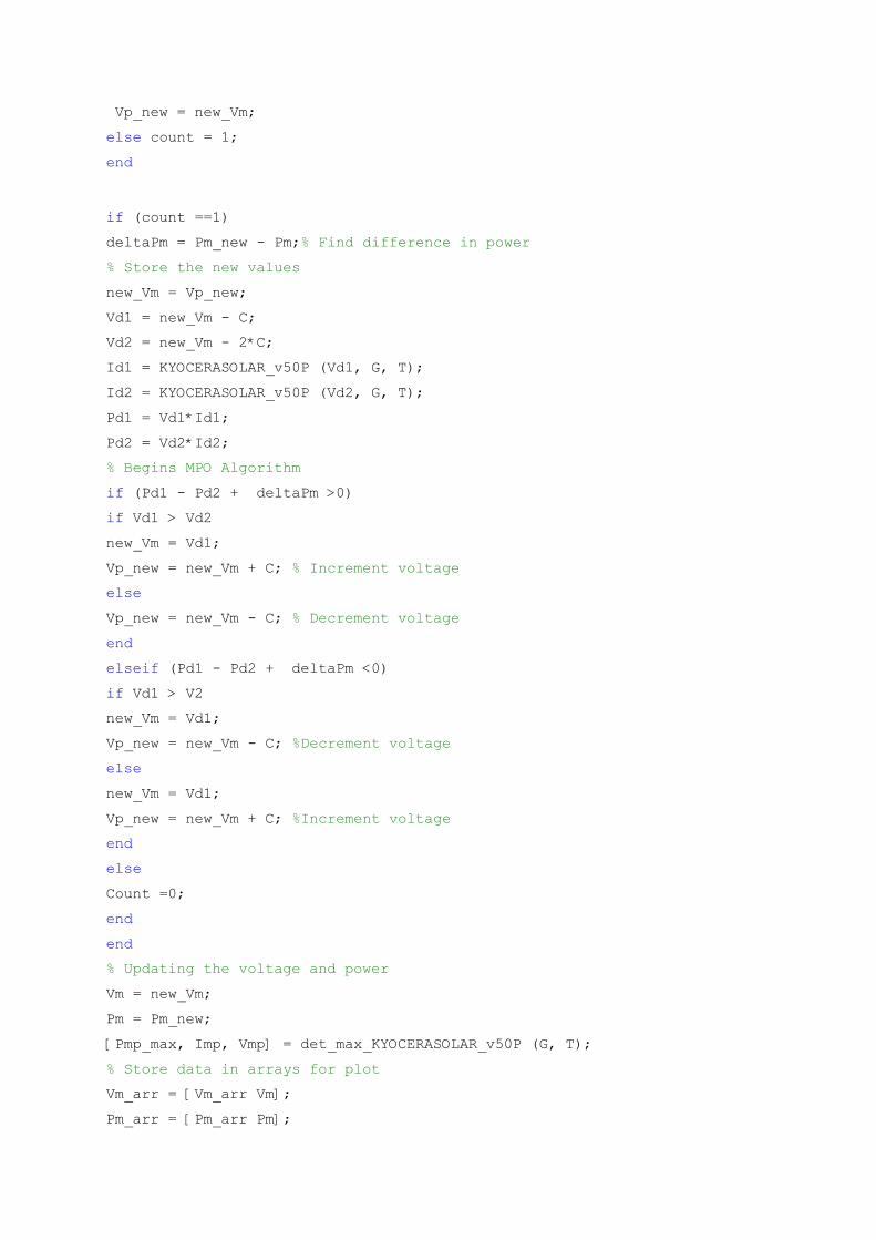
Vp_new = new_Vm;
else count = 1;
end
if (count ==1)
deltaPm = Pm_new - Pm;% Find difference in power
% Store the new values
new_Vm = Vp_new;
Vd1 = new_Vm - C;
Vd2 = new_Vm - 2*C;
Id1 = KYOCERASOLAR_v50P (Vd1, G, T);
Id2 = KYOCERASOLAR_v50P (Vd2, G, T);
Pd1 = Vd1*Id1;
Pd2 = Vd2*Id2;
% Begins MPO Algorithm
if (Pd1 - Pd2 + deltaPm >0)
if Vd1 > Vd2
new_Vm = Vd1;
Vp_new = new_Vm + C; % Increment voltage
else
Vp_new = new_Vm - C; % Decrement voltage
end
elseif (Pd1 - Pd2 + deltaPm <0)
if Vd1 > V2
new_Vm = Vd1;
Vp_new = new_Vm - C; %Decrement voltage
else
new_Vm = Vd1;
Vp_new = new_Vm + C; %Increment voltage
end
else
Count =0;
end
end
% Updating the voltage and power
Vm = new_Vm;
Pm = Pm_new;
[Pmp_max, Imp, Vmp] = det_max_KYOCERASOLAR_v50P (G, T);
% Store data in arrays for plot
Vm_arr = [Vm_arr Vm];
Pm_arr = [Pm_arr Pm];
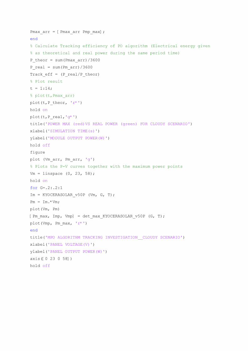
Pmax_arr = [Pmax_arr Pmp_max];
end
% Calculate Tracking efficiency of PO algorithm (Electrical energy given
% as theoretical and real power during the same period time)
P_theor = sum(Pmax_arr)/3600
P_real = sum(Pm_arr)/3600
Track_eff = (P_real/P_theor)
% Plot result
t = 1:14;
% plot(t,Pmax_arr)
plot(t,P_theor, 'r*')
hold on
plot(t,P_real,'g*')
title('POWER MAX (red)VS REAL POWER (green) FOR CLOUDY SCENARIO')
xlabel('SIMULATION TIME(s)')
ylabel('MODULE OUTPUT POWER(W)')
hold off
figure
plot (Vm_arr, Pm_arr, 'g')
% Plots the P-V curves together with the maximum power points
Vm = linspace (0, 23, 58);
hold on
for G=.2:.2:1
Im = KYOCERASOLAR_v50P (Vm, G, T);
Pm = Im.*Vm;
plot(Vm, Pm)
[Pm_max, Imp, Vmp] = det_max_KYOCERASOLAR_v50P (G, T);
plot(Vmp, Pm_max, 'r*')
end
title('MPO ALGORITHM TRACKING INVESTIGATION__CLOUDY SCENARIO')
xlabel('PANEL VOLTAGE(V)')
ylabel('PANEL OUTPUT POWER(W)')
axis([0 23 0 58])
hold off

MATLAB m-files script Code for calculating the maximum operating power of
modified PO algorithm version 2 (EPP) under atmospheric sunny conditions
% MATLAB Script file for investigating the PO MPPT Algorithm modified
% version 2 (or EPP) under sunny weather conditions
%( Slowly change of solar irradiance G)
% Created by Cedrick, February, 2011
%%%%%%%%%%%%%%%%%%%%%%%%%%%%%%%%%%%%%%%%%%%%%%%%%%%%%%%%%%%%%%
Clear;
Global T % makes variable T accessible on a global scope
% Initial Conditions
T = 25; % Temperature of the solar panel cell (C)
C = 0.1; % increment voltage (V)
G = 0.025; % solar irradiance
Vm = 17.3; % panel voltage (V)
Im = KYOCERASOLAR_v50P (Vm, G,T);% PV current of module
Pm = Vm * Im; % Panel power output
Vp_new = Vm + C; % updated reference panel voltage
% Create vectors for voltage and power data
Vm_arr = [];
Pm_arr = [];
Pmax_arr = [];
% Provide irradiance data for a sunny day at Upington
% Data stored in a 14 by 2 matrix, with column 1 being the time data and
% column 2 the irradiation data
G_data = [1 0.02; 2 0.204; 3 0.439; 4 0.664; 5 0.827; 6 0.981; 7 1.073; ...
8 1.073; 9 1; 10 0.868; 11 0.684; 12 0.449; 13 0.214; 14 0.03];
x_t = G_data(:,1)'; % Store time data in vector x_t (hour)
y_G = G_data(:,2)'; % Store irradiation data in vector y_G (Kw/m2)
x_ti = 1: 300; % Creates a 1 by 300 vector for interpolation
y_Gi = interp1 (x_t, y_G, x_ti,'linear'); % Perform linear interpolation
% Initialization
Count = 0;
for i = 1:14
G = y_Gi (i); %Store interpolated values
new_Vm = Vp_new; %measure voltage
new_Im = KYOCERASOLAR_v50P (Vp_new, G,T);% measure current
Pm_new = new_Vm * new_Im;% Determine new power
% deltaPm = Pm_new - Pm;
if (count == 0)
Vp_new = new_Vm;
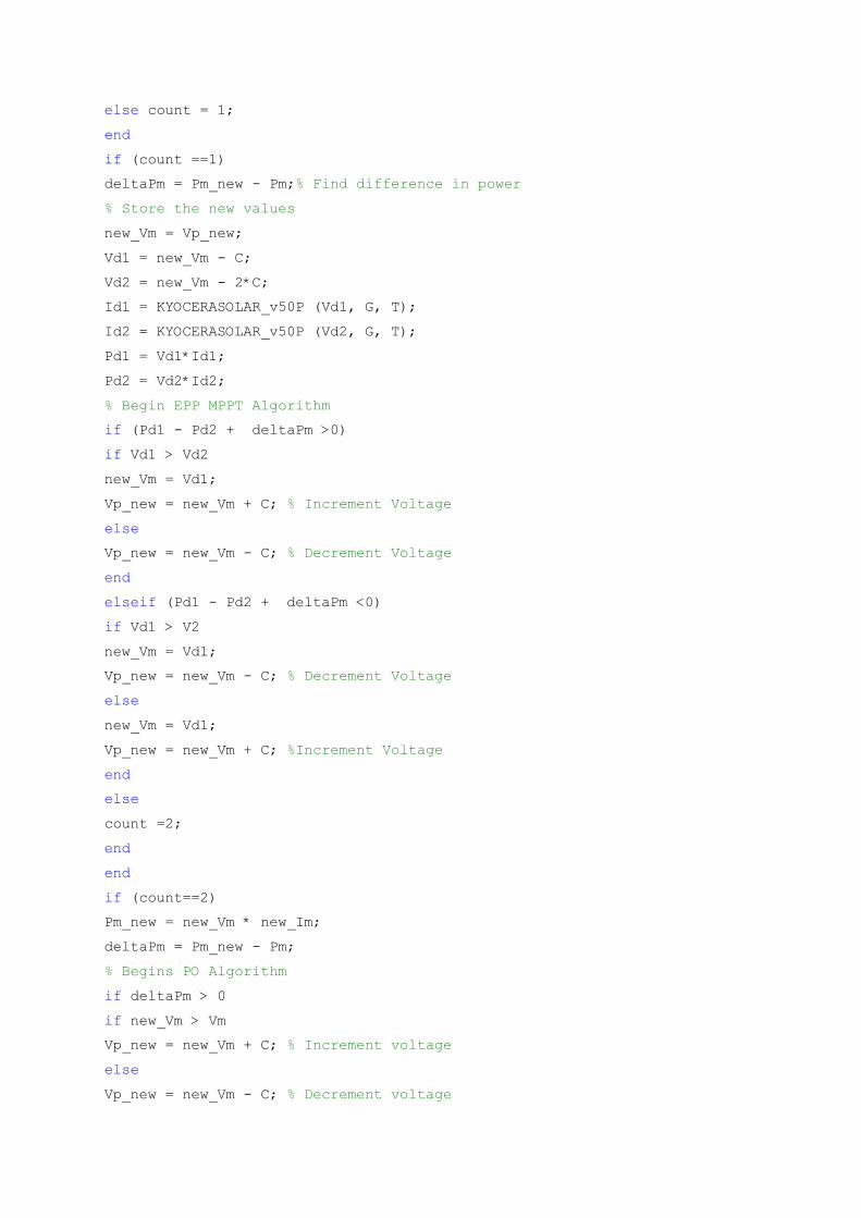
else count = 1;
end
if (count ==1)
deltaPm = Pm_new - Pm;% Find difference in power
% Store the new values
new_Vm = Vp_new;
Vd1 = new_Vm - C;
Vd2 = new_Vm - 2*C;
Id1 = KYOCERASOLAR_v50P (Vd1, G, T);
Id2 = KYOCERASOLAR_v50P (Vd2, G, T);
Pd1 = Vd1*Id1;
Pd2 = Vd2*Id2;
% Begin EPP MPPT Algorithm
if (Pd1 - Pd2 + deltaPm >0)
if Vd1 > Vd2
new_Vm = Vd1;
Vp_new = new_Vm + C; % Increment Voltage
else
Vp_new = new_Vm - C; % Decrement Voltage
end
elseif (Pd1 - Pd2 + deltaPm <0)
if Vd1 > V2
new_Vm = Vd1;
Vp_new = new_Vm - C; % Decrement Voltage
else
new_Vm = Vd1;
Vp_new = new_Vm + C; %Increment Voltage
end
else
count =2;
end
end
if (count==2)
Pm_new = new_Vm * new_Im;
deltaPm = Pm_new - Pm;
% Begins PO Algorithm
if deltaPm > 0
if new_Vm > Vm
Vp_new = new_Vm + C; % Increment voltage
else
Vp_new = new_Vm - C; % Decrement voltage
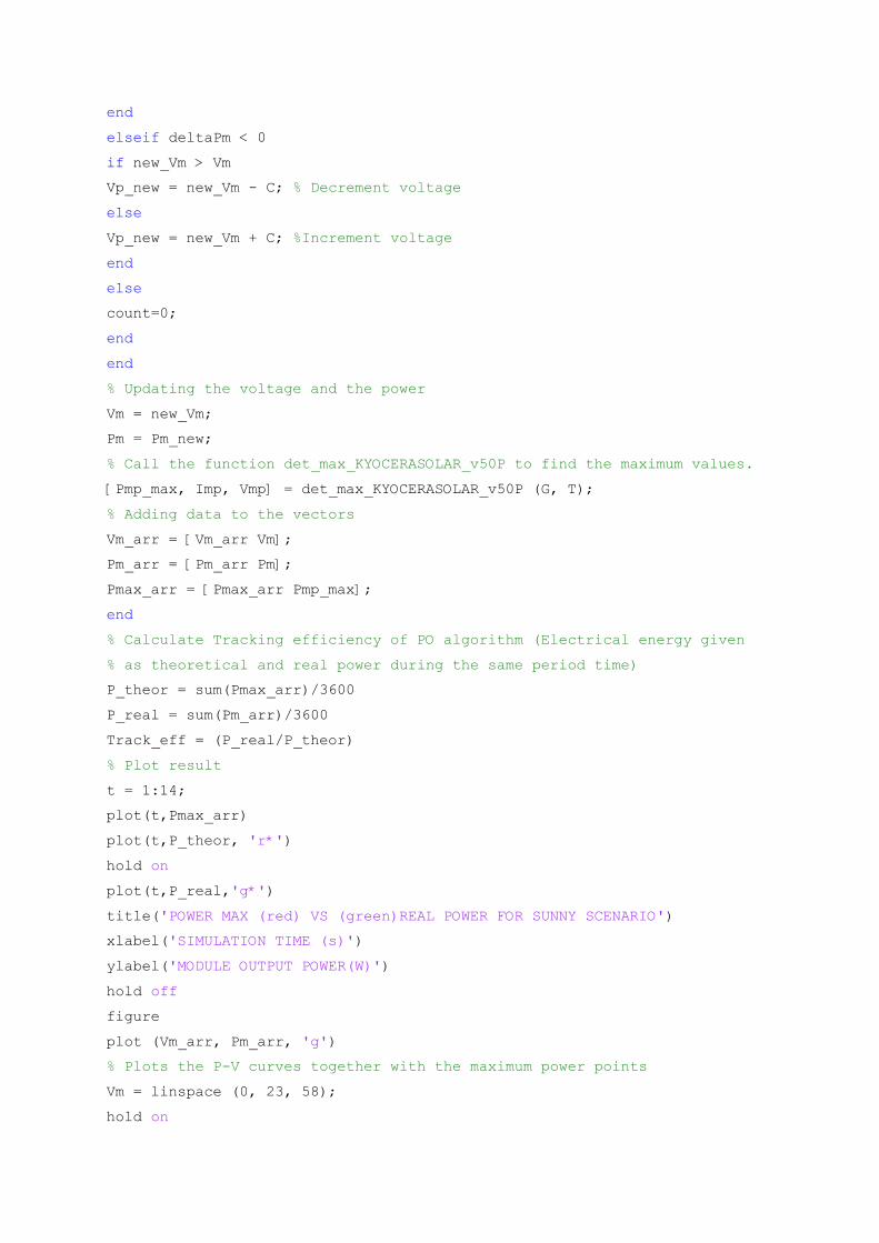
end
elseif deltaPm < 0
if new_Vm > Vm
Vp_new = new_Vm - C; % Decrement voltage
else
Vp_new = new_Vm + C; %Increment voltage
end
else
count=0;
end
end
% Updating the voltage and the power
Vm = new_Vm;
Pm = Pm_new;
% Call the function det_max_KYOCERASOLAR_v50P to find the maximum values.
[Pmp_max, Imp, Vmp] = det_max_KYOCERASOLAR_v50P (G, T);
% Adding data to the vectors
Vm_arr = [Vm_arr Vm];
Pm_arr = [Pm_arr Pm];
Pmax_arr = [Pmax_arr Pmp_max];
end
% Calculate Tracking efficiency of PO algorithm (Electrical energy given
% as theoretical and real power during the same period time)
P_theor = sum(Pmax_arr)/3600
P_real = sum(Pm_arr)/3600
Track_eff = (P_real/P_theor)
% Plot result
t = 1:14;
plot(t,Pmax_arr)
plot(t,P_theor, 'r*')
hold on
plot(t,P_real,'g*')
title('POWER MAX (red) VS (green)REAL POWER FOR SUNNY SCENARIO')
xlabel('SIMULATION TIME (s)')
ylabel('MODULE OUTPUT POWER(W)')
hold off
figure
plot (Vm_arr, Pm_arr, 'g')
% Plots the P-V curves together with the maximum power points
Vm = linspace (0, 23, 58);
hold on

for G=.2:.2:1
Im = KYOCERASOLAR_v50P (Vm, G, T);
Pm = Im.*Vm;
plot(Vm, Pm)
% plot(G, Pm,'r*')
[Pm_max, Imp, Vmp] = det_max_KYOCERASOLAR_v50P (G, T);
plot(Vmp, Pm_max, 'r*')
end
title('EPP ALGORITHM TRACKING INVESTIGATION__SUNNY SCENARIO')
xlabel('PANEL VOLTAGE (V)')
ylabel('PANEL OUTPUT POWER(W)')
axis([0 23 0 58])
hold off

MATLAB m-files script Code for calculating the maximum operating power of IC
algorithm under atmospheric sunny conditions
%MATLAB Script file for investigating the IC MPPT Algorithm under
% sunny weather conditions (slowly change of solar irradiance G)
% Created by Cedrick, February, 2011
%///////////////////////////////////////////////////////////////////////
Clear;
Global T % makes variable T accessible on a global scope
% Initialize constants
T = 25; % Temperature of the solar panel cell (C)
C = 0.1; % increment voltage (V)
err = 0.0217; % max error
G = 0.025; % solar irradiance
Vm = 17.3; % panel voltage
Im = KYOCERASOLAR_v50P (Vm, G, T); % PV current of module
Pm = Vm * Im; % Panel power output
Vp_new = Vm + C; % updated reference panel voltage
% Create vectors for voltage and power data
Vm_arr = [];
Pm_arr = [];
Pmax_arr = [];
% Provide solar irradiation data for a sunny day at Upington
% Data stored in a 14 by 2 matrix, with column 1 being the time data and
% column 2 the irradiation data
G_data = [1 0.02; 2 0.204; 3 0.439; 4 0.664; 5 0.827; 6 0.981; 7 1.073; ...
8 1.073; 9 1; 10 0.868; 11 0.684; 12 0.449; 13 0.214; 14 0.03];
x_t = G_data(:,1)'; % Store time data in vector x_t (hour)
y_G = G_data(:,2)'; % Store irradiation data in vector y_G (Kw/m2)
x_ti = 1: 300; % Creates a 1 by 300 vector for interpolation
y_Gi = interp1 (x_t, y_G, x_ti,'linear'); % Perform linear interpolation
for i = 1:14
G = y_Gi (i); % Store interpolated values
new_Vm = Vp_new;% measure voltage
new_Im = KYOCERASOLAR_v50P (Vp_new, G, T); %measure current
% Find the difference in voltage and current
deltaVm = new_Vm - Vm;
deltaIm = new_Im - Im;
%Begins IC Algorithm
if deltaVm == 0
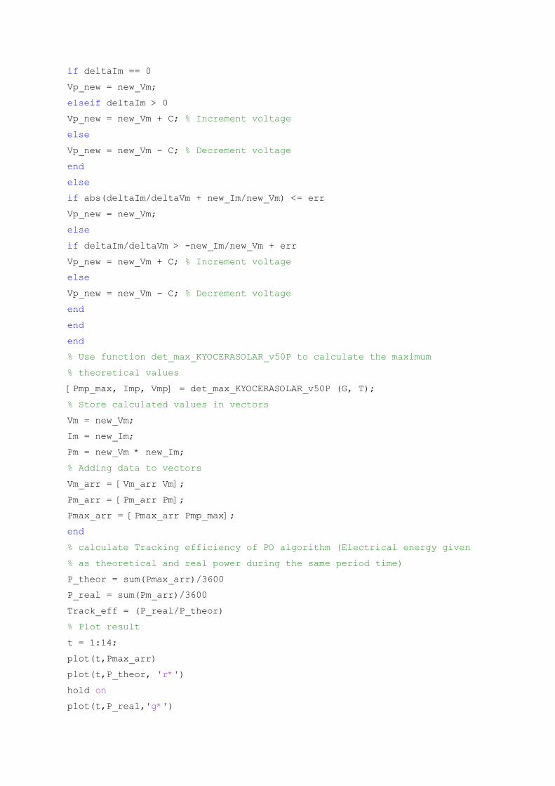
if deltaIm == 0
Vp_new = new_Vm;
elseif deltaIm > 0
Vp_new = new_Vm + C; % Increment voltage
else
Vp_new = new_Vm - C; % Decrement voltage
end
else
if abs(deltaIm/deltaVm + new_Im/new_Vm) <= err
Vp_new = new_Vm;
else
if deltaIm/deltaVm > -new_Im/new_Vm + err
Vp_new = new_Vm + C; % Increment voltage
else
Vp_new = new_Vm - C; % Decrement voltage
end
end
end
% Use function det_max_KYOCERASOLAR_v50P to calculate the maximum
% theoretical values
[Pmp_max, Imp, Vmp] = det_max_KYOCERASOLAR_v50P (G, T);
% Store calculated values in vectors
Vm = new_Vm;
Im = new_Im;
Pm = new_Vm * new_Im;
% Adding data to vectors
Vm_arr = [Vm_arr Vm];
Pm_arr = [Pm_arr Pm];
Pmax_arr = [Pmax_arr Pmp_max];
end
% calculate Tracking efficiency of PO algorithm (Electrical energy given
% as theoretical and real power during the same period time)
P_theor = sum(Pmax_arr)/3600
P_real = sum(Pm_arr)/3600
Track_eff = (P_real/P_theor)
% Plot result
t = 1:14;
plot(t,Pmax_arr)
plot(t,P_theor, 'r*')
hold on
plot(t,P_real,'g*')

title('POWER MAX (red) VS (green)REAL POWER FOR SUNNY SCENARIO')
xlabel('SIMULATION TIME (s)')
ylabel('MODULE OUTPUT POWER (W)')
hold off
figure
plot (Vm_arr, Pm_arr, 'g')
% Plots the P-V curves together with the maximum power points
Vm = linspace (0, 23, 58);
hold on
for G=.2:.2:1
Im = KYOCERASOLAR_v50P (Vm, G, T);
Pm = Im.*Vm;
plot(Vm, Pm)
[Pm_max, Imp, Vmp] = det_max_KYOCERASOLAR_v50P (G, T);
plot(Vmp, Pm_max, 'r*')
end
title('IC ALGORITHM TRACKING INVESTIGATION__SUNNY SCENARIO')
xlabel('PANEL VOLTAGE (V)')
ylabel('PANEL POWER OUTPUT (W)')
axis([0 23 0 58])
hold off

MATLAB m-files script Code for calculating the maximum operating power of the
modified CV- IC two-mode algorithm under atmospheric cloudy conditions
%MATLAB Script files for investigating the two-stage CV-IC MPPT Algorithm
%under cloudy weather conditions (rapidly change of solar irradiance G)
% Created by Cedrick, February, 2011
%///////////////////////////////////////////////////////////////////////
Clear;
Global T% makes variable T accessible on a global scope
% Initialize constants
C = 0.0025; % increment voltage (V)
T = 25; % Temperature of the solar panel cell (C)
err = 0.0217; % max error
G = 0.025; % solar irradiance
Vm = 17.3; % panel voltage
Im = KYOCERASOLAR_v50P (Vm, G, T); % PV current of module
Pm = Vm * Im; % Panel power output
Voc = 22.1; % datasheet open circuit voltage
k = 0.765; %constant in Constant Voltage (CV) MPPT method
Vp_new = Vm + C; % updated reference panel voltage
% Create vectors for voltage and power data
Vm_arr = [];
Pm_arr = [];
Pmax_arr = [];
%Provide Irradiation data for a cloudy day at upington (South Africa)
% Data stored in a 14 by 2 matrix, with column 1 being the time data and
% column 2 the irradiation data
G_data = [1 0.03; 2 0.143; 3 0.163; 4 0.613; 5 0.725; 6 0.245; 7 0.388;...
8 0.347; 9 0.449; 10 0.521; 11 0.357; 12 0.388; 13 0.163; 14 0.082];
x_t = G_data (:,1)'; % Store time data in vector x_t (hour)
y_G = G_data (:,2)'; % Store irradiation data in vector y_G (Kw/m2)
x_ti = 1: 300; % Creates a 1 by 300 vector for interpolation
y_Gi = interp1 (x_t, y_G, x_ti,'linear'); % Perform linear interpolation
for i = 1:14
G = y_Gi (i); %Store interpolated values
new_Vm = Vp_new; % measure voltage
new_Im = KYOCERASOLAR_v50P (Vp_new, G,T);%measure current
deltaIm = new_Im - Im;
if ((deltaIm/Im)<0.33)
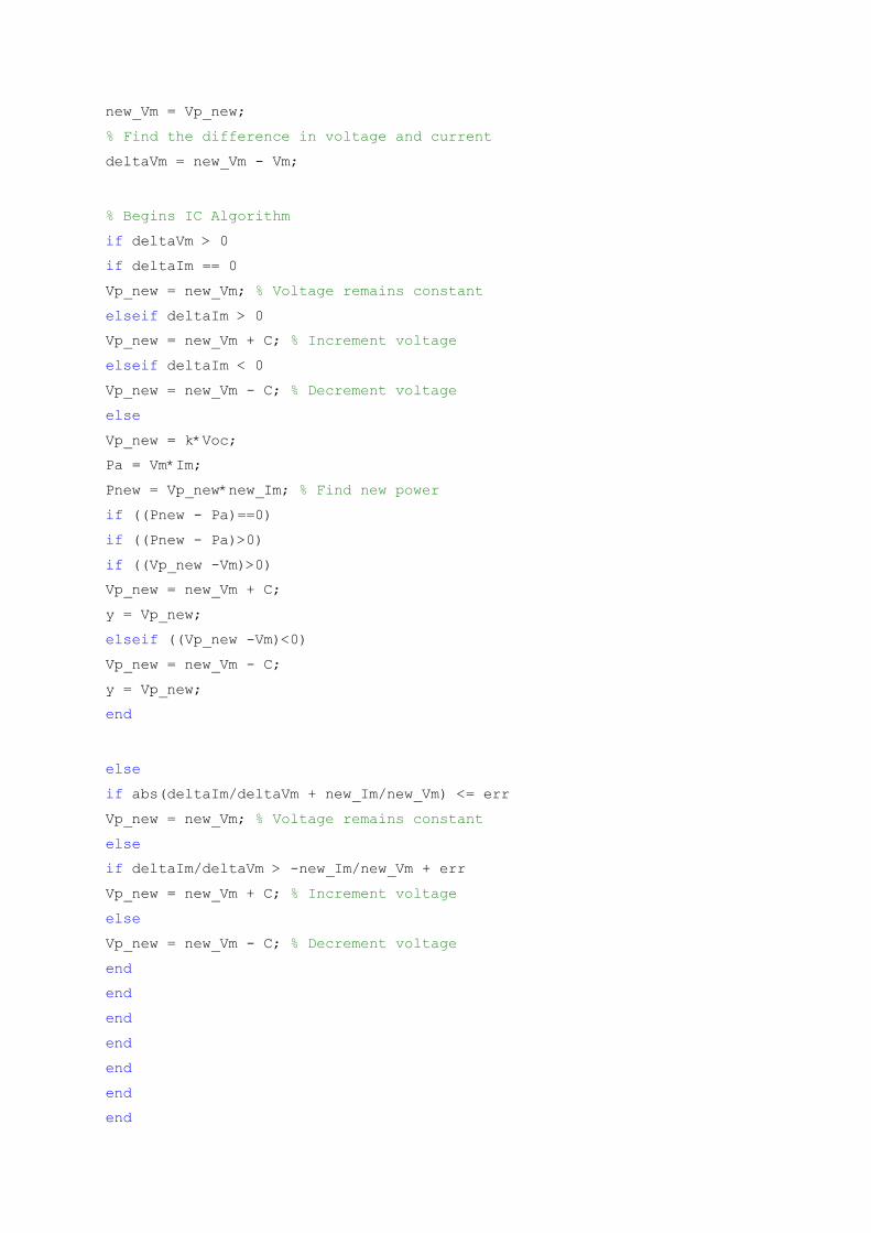
new_Vm = Vp_new;
% Find the difference in voltage and current
deltaVm = new_Vm - Vm;
% Begins IC Algorithm
if deltaVm > 0
if deltaIm == 0
Vp_new = new_Vm; % Voltage remains constant
elseif deltaIm > 0
Vp_new = new_Vm + C; % Increment voltage
elseif deltaIm < 0
Vp_new = new_Vm - C; % Decrement voltage
else
Vp_new = k*Voc;
Pa = Vm*Im;
Pnew = Vp_new*new_Im; % Find new power
if ((Pnew - Pa)==0)
if ((Pnew - Pa)>0)
if ((Vp_new -Vm)>0)
Vp_new = new_Vm + C;
y = Vp_new;
elseif ((Vp_new -Vm)<0)
Vp_new = new_Vm - C;
y = Vp_new;
end
else
if abs(deltaIm/deltaVm + new_Im/new_Vm) <= err
Vp_new = new_Vm; % Voltage remains constant
else
if deltaIm/deltaVm > -new_Im/new_Vm + err
Vp_new = new_Vm + C; % Increment voltage
else
Vp_new = new_Vm - C; % Decrement voltage
end
end
end
end
end
end
end
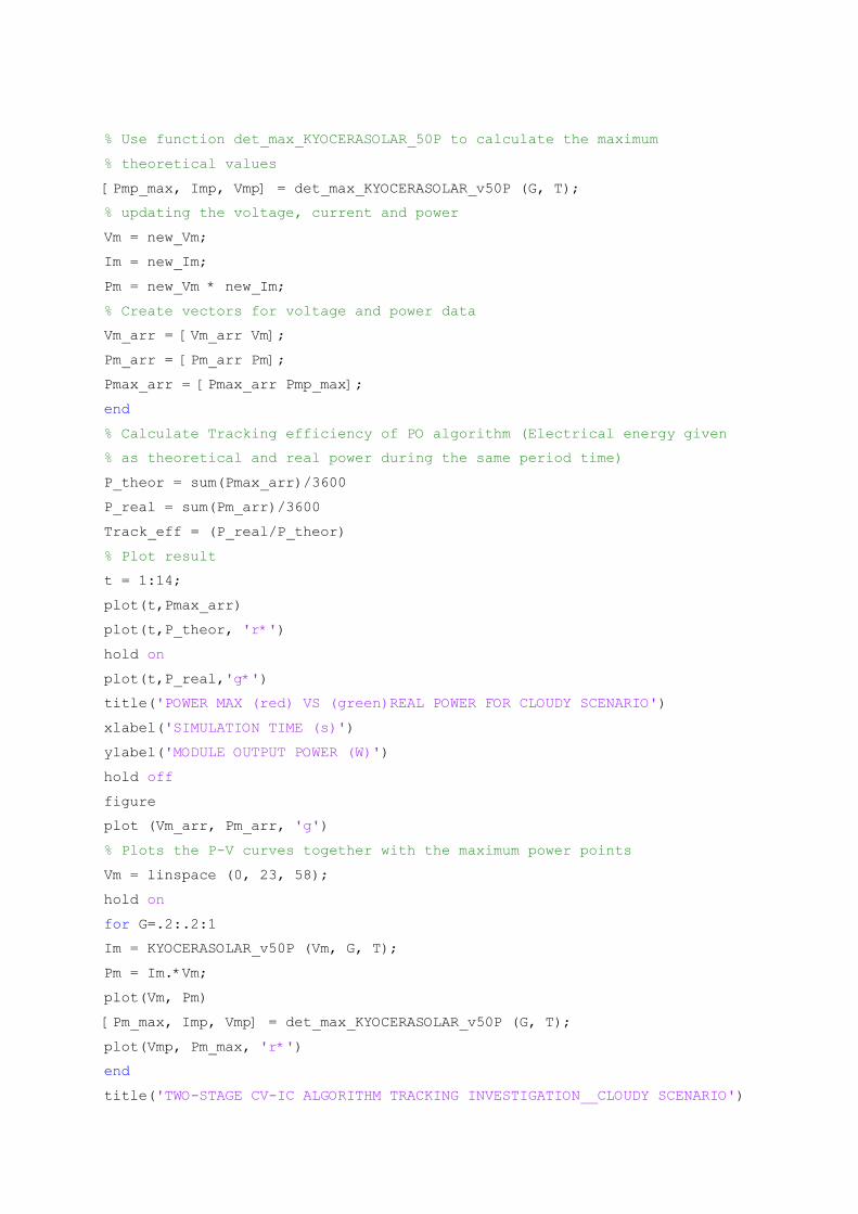
% Use function det_max_KYOCERASOLAR_50P to calculate the maximum
% theoretical values
[Pmp_max, Imp, Vmp] = det_max_KYOCERASOLAR_v50P (G, T);
% updating the voltage, current and power
Vm = new_Vm;
Im = new_Im;
Pm = new_Vm * new_Im;
% Create vectors for voltage and power data
Vm_arr = [Vm_arr Vm];
Pm_arr = [Pm_arr Pm];
Pmax_arr = [Pmax_arr Pmp_max];
end
% Calculate Tracking efficiency of PO algorithm (Electrical energy given
% as theoretical and real power during the same period time)
P_theor = sum(Pmax_arr)/3600
P_real = sum(Pm_arr)/3600
Track_eff = (P_real/P_theor)
% Plot result
t = 1:14;
plot(t,Pmax_arr)
plot(t,P_theor, 'r*')
hold on
plot(t,P_real,'g*')
title('POWER MAX (red) VS (green)REAL POWER FOR CLOUDY SCENARIO')
xlabel('SIMULATION TIME (s)')
ylabel('MODULE OUTPUT POWER (W)')
hold off
figure
plot (Vm_arr, Pm_arr, 'g')
% Plots the P-V curves together with the maximum power points
Vm = linspace (0, 23, 58);
hold on
for G=.2:.2:1
Im = KYOCERASOLAR_v50P (Vm, G, T);
Pm = Im.*Vm;
plot(Vm, Pm)
[Pm_max, Imp, Vmp] = det_max_KYOCERASOLAR_v50P (G, T);
plot(Vmp, Pm_max, 'r*')
end
title('TWO-STAGE CV-IC ALGORITHM TRACKING INVESTIGATION__CLOUDY SCENARIO')

xlabel('MODULE VOLTAGE (V)')
ylabel('MMODULE OUTPUT POWER (W)')
axis([0 23 0 58])
hold off
Measurement of cloudy and sunny irradiation data in Upington, South Africa, 1966
(KJ/m2/hour) [35]
Sunny scenario: 6 February 1966
[0 0 0 0 0 73 735 1582 2391 2980 3532 3863 3863 3605 3127 2465 1618 772 11 0 0 0 0 0] Cloudy scenario: 11 January 1966 [0 0 0 0 0 110 515 588 2207 2612 883 1398 1250 1618 1876 1287 1398 588 294 0 0 0 0 0]
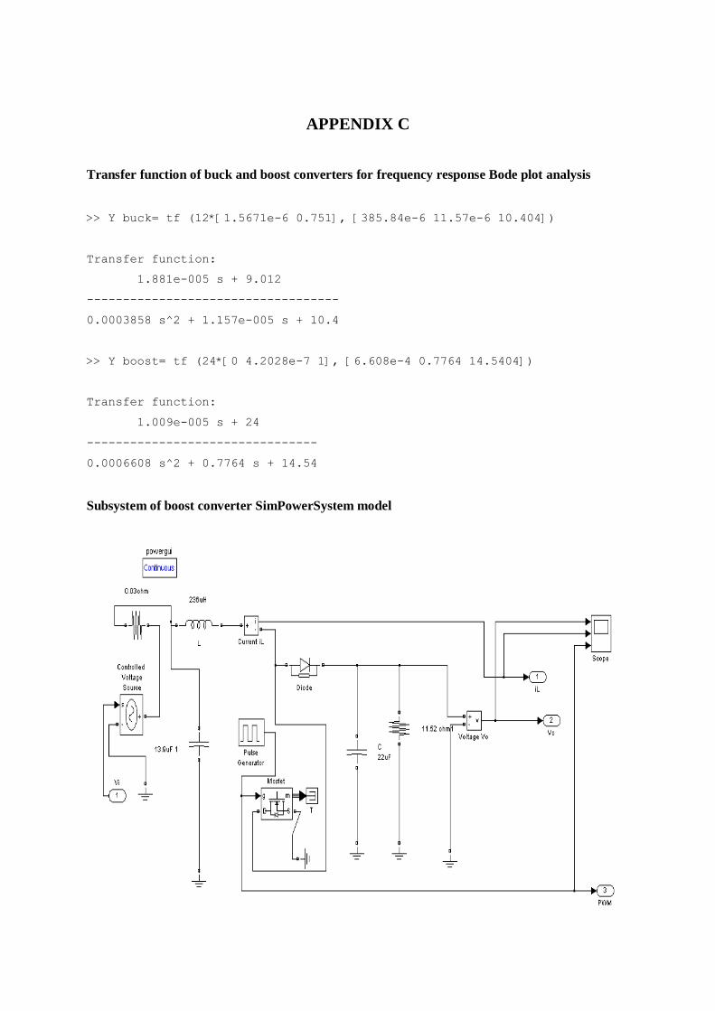
APPENDIX C Transfer function of buck and boost converters for frequency response Bode plot analysis
>> Y buck= tf (12*[1.5671e-6 0.751], [385.84e-6 11.57e-6 10.404])
Transfer function:
1.881e-005 s + 9.012
-----------------------------------
0.0003858 s^2 + 1.157e-005 s + 10.4
>> Y boost= tf (24*[0 4.2028e-7 1], [6.608e-4 0.7764 14.5404])
Transfer function:
1.009e-005 s + 24
--------------------------------
0.0006608 s^2 + 0.7764 s + 14.54
Subsystem of boost converter SimPowerSystem model
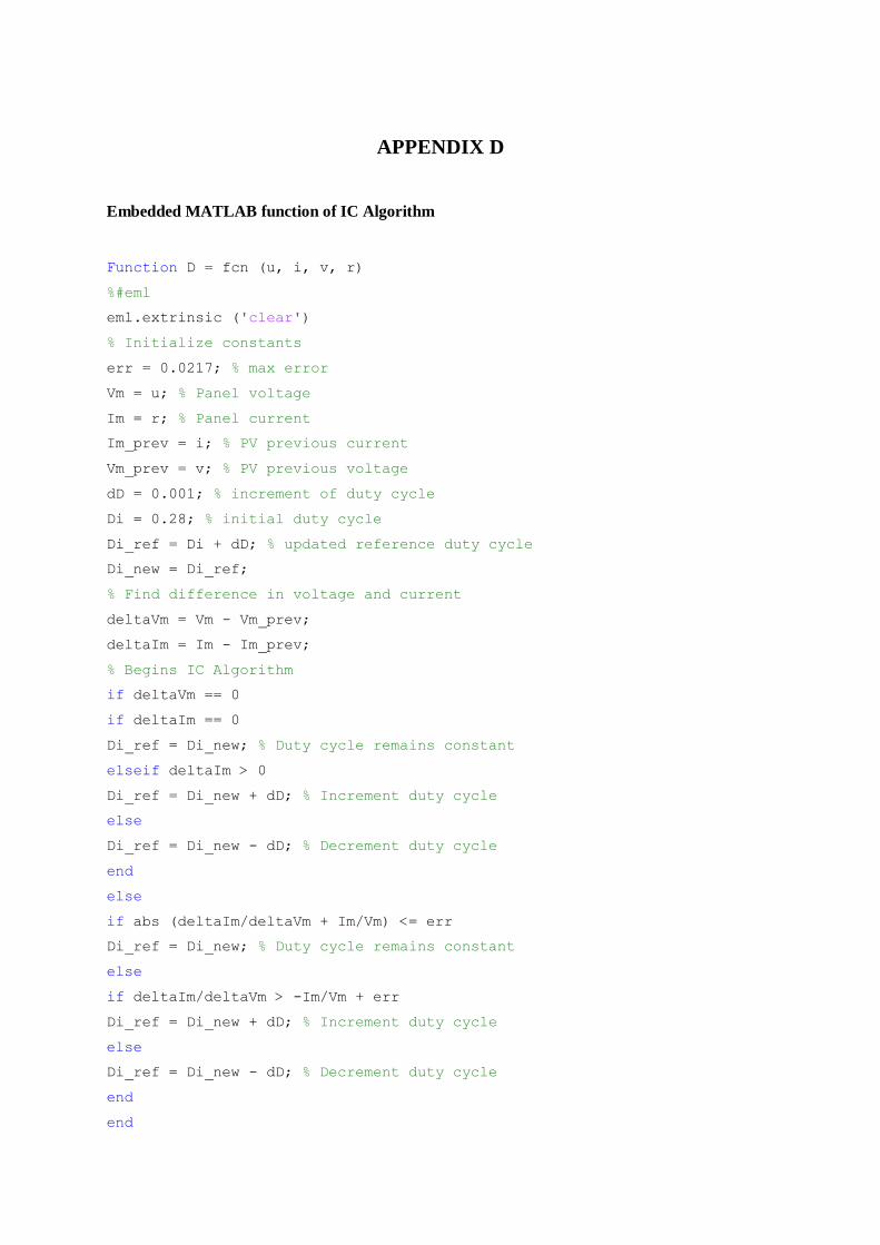
APPENDIX D
Embedded MATLAB function of IC Algorithm
Function D = fcn (u, i, v, r)
%#eml
eml.extrinsic ('clear')
% Initialize constants
err = 0.0217; % max error
Vm = u; % Panel voltage
Im = r; % Panel current
Im_prev = i; % PV previous current
Vm_prev = v; % PV previous voltage
dD = 0.001; % increment of duty cycle
Di = 0.28; % initial duty cycle
Di_ref = Di + dD; % updated reference duty cycle
Di_new = Di_ref;
% Find difference in voltage and current
deltaVm = Vm - Vm_prev;
deltaIm = Im - Im_prev;
% Begins IC Algorithm
if deltaVm == 0
if deltaIm == 0
Di_ref = Di_new; % Duty cycle remains constant
elseif deltaIm > 0
Di_ref = Di_new + dD; % Increment duty cycle
else
Di_ref = Di_new - dD; % Decrement duty cycle
end
else
if abs (deltaIm/deltaVm + Im/Vm) <= err
Di_ref = Di_new; % Duty cycle remains constant
else
if deltaIm/deltaVm > -Im/Vm + err
Di_ref = Di_new + dD; % Increment duty cycle
else
Di_ref = Di_new - dD; % Decrement duty cycle
end
end

end
D = Di_ref;
end
Embedded MATLAB function of two-stage CV-IC Algorithm
Function D = fcn (u, i, v, r)
%#eml
eml.extrinsic ('clear')
% Initialize constants
Voc = 22.1; %datasheet open circuit voltage
k = 0.765; % constant in CV MPPT method
err = 0.0217; % error max
dD = 0.0001; % increment of duty cycle
Di = 0.28; % initial duty cycle
Vm = u; % Panel voltage
Im_prev = I; % Previous Panel current
Vm_prev = v; % Previous Panel voltage
Di_ref = Di + dD; % Updated reference duty cycle
D = Di_ref;
Im = r;
% Find difference in current
deltaIm = Im - Im_prev;
if ((deltaIm/Im)<0.33)
Di_new = Di_ref;
% Find difference in voltage
deltaVm = Vm - Vm_prev;
% Begins Two-mode CV-IC Algorithm
if deltaVm > 0
if deltaIm == 0
Di_ref = Di_new; % Duty cycle remains constant
D = Di_ref;
elseif deltaIm > 0
Di_ref = Di_new + dD; % Increment duty cycle
D = Di_ref;
elseif deltaIm < 0
Di_ref = Di_new - dD; % Decrement duty cycle
D = Di_ref;
else
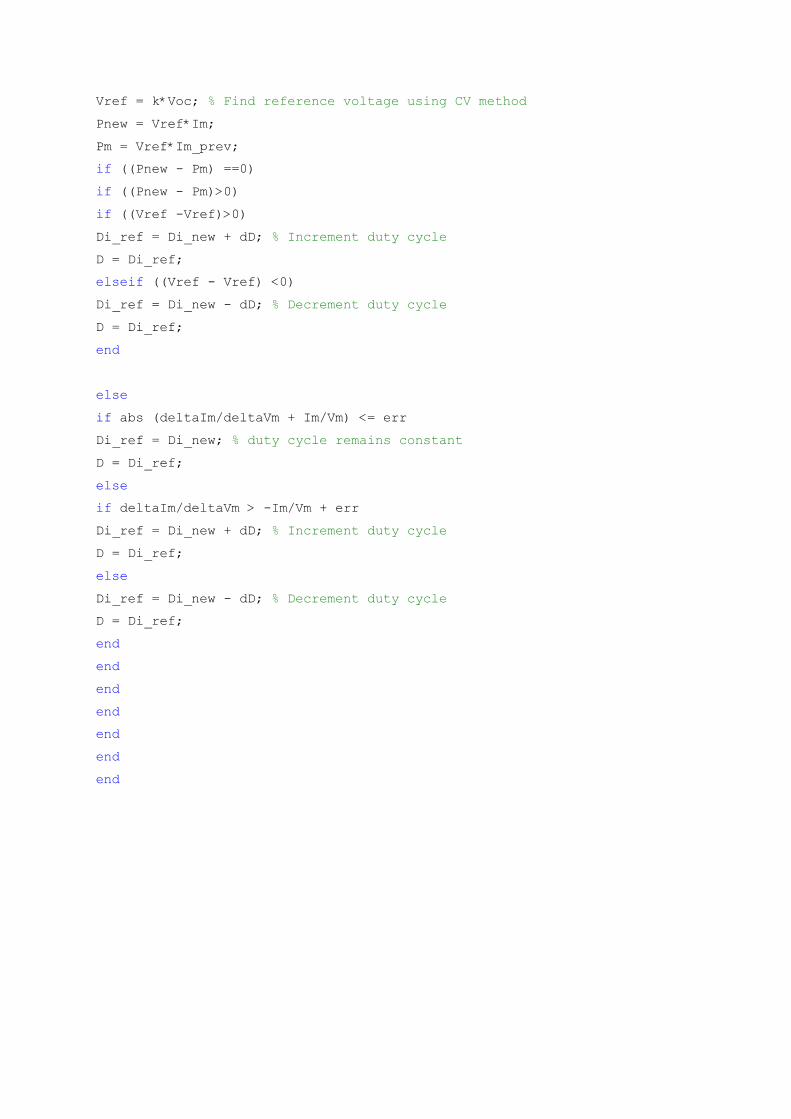
Vref = k*Voc; % Find reference voltage using CV method
Pnew = Vref*Im;
Pm = Vref*Im_prev;
if ((Pnew - Pm) ==0)
if ((Pnew - Pm)>0)
if ((Vref -Vref)>0)
Di_ref = Di_new + dD; % Increment duty cycle
D = Di_ref;
elseif ((Vref - Vref) <0)
Di_ref = Di_new - dD; % Decrement duty cycle
D = Di_ref;
end
else
if abs (deltaIm/deltaVm + Im/Vm) <= err
Di_ref = Di_new; % duty cycle remains constant
D = Di_ref;
else
if deltaIm/deltaVm > -Im/Vm + err
Di_ref = Di_new + dD; % Increment duty cycle
D = Di_ref;
else
Di_ref = Di_new - dD; % Decrement duty cycle
D = Di_ref;
end
end
end
end
end
end
end
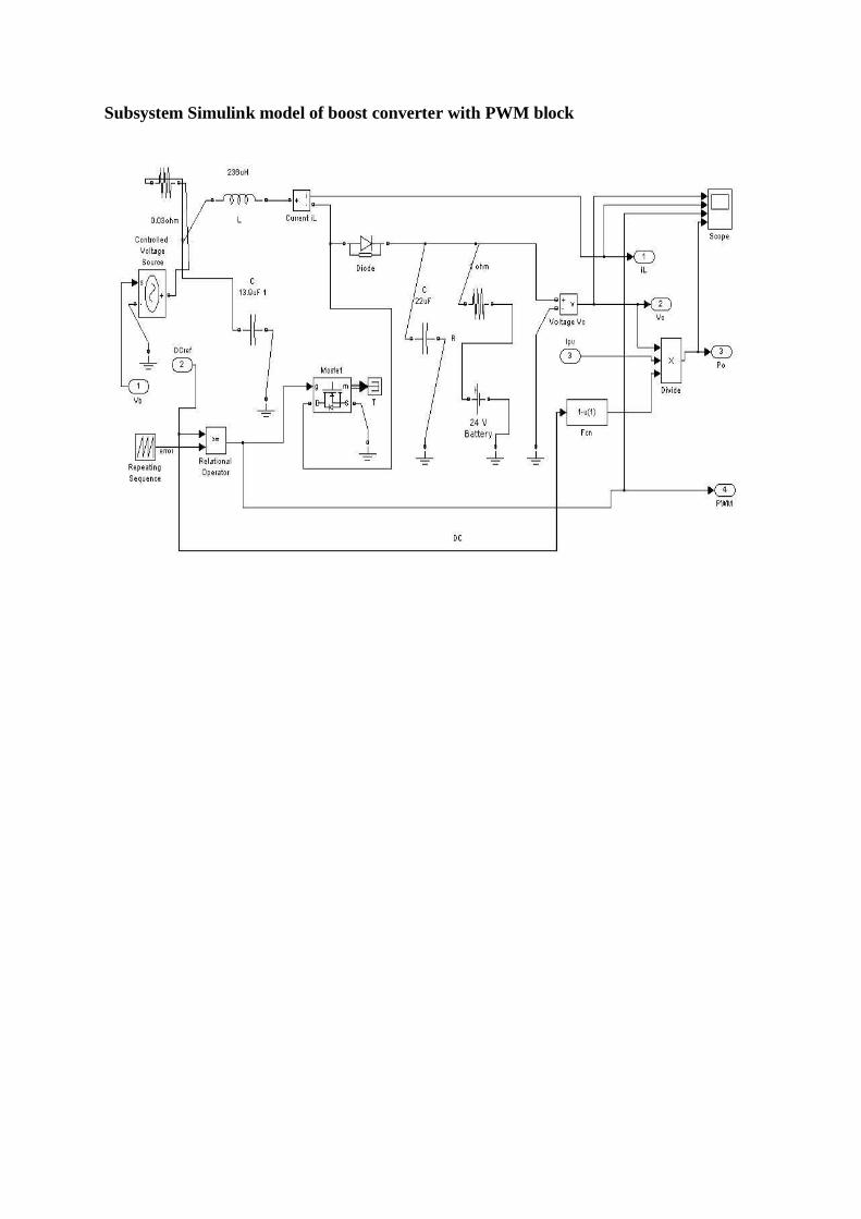
Subsystem Simulink model of boost converter with PWM block
236uH
...f"'{)'Q'1}\---+
d;;b Diode
13.9uF 1
DC ref +I -±-
-±-Sequence
l "'J Battery
-±- -±-
DC
iL
Divide
Fen
Scope
4
PWM
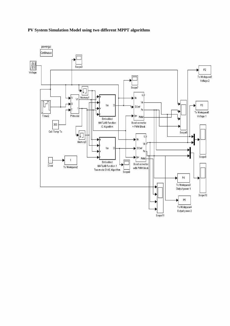
PV System Simulation Model using two different MPPT algorithms
Scope3
Voltage
Cell Temp Tc
D..._____~~-~1 Clock T 0 Wolkspace2
fen 0
Embedded MAT LAB Function
IC Algorilhm
fen 0
Embedded MAT LAB Function 1
Two-mode CV-IC Algorithm Scope9
Scope7
il
IA>L----
Boost converter + PWM Block
Scope11
To Wolkspace4 Output power 2
To Wolkspace5 Voltage 2
To Wolkspace6 Voltage 1
Scope10


