Embed Size (px)
Citation preview

P-06-32
Oskarshamn site investigation
Borehole KLX08
Uniaxial compression test of intact rock
Lars Jacobsson
SP Swedish National Testing and Research Institute
October 2006
Svensk Kärnbränslehantering ABSwedish Nuclear Fueland Waste Management CoBox 5864SE-102 40 Stockholm Sweden Tel 08-459 84 00 +46 8 459 84 00Fax 08-661 57 19 +46 8 661 57 19
CM
Gru
ppen
AB
, Bro
mm
a, 2
007

ISSN 1651-4416
SKB P-06-32
Oskarshamn site investigation
Borehole KLX08
Uniaxial compression test of intact rock
Lars Jacobsson
SP Swedish National Testing and Research Institute
October 2006
Keywords: Rock mechanics, Uniaxial compression test, Elasticity parameters, Stress-strain curve, Post-failure behaviour, AP PS 400-05-085.
This report concerns a study which was conducted for SKB. The conclusions and viewpoints presented in the report are those of the author and do not necessarily coincide with those of the client.
A pdf version of this document can be downloaded from www.skb.se

�
Abstract
Uniaxial compression tests, containing the complete loading response beyond compressive fail-ure, so called post-failure tests, were carried out on 6 water saturated specimens of intact rock from borehole KLX08 in Oskarshamn. The cylindrical specimens were taken from drill cores at three depth levels ranging between 586–610 m, 689–692 m respectively 841 m borehole length. The collected rock type was diorite-gabbro in all specimens. The elastic properties, represented by Young’s modulus and the Poisson ratio, and the uniaxial compressive strength were deduced from these tests. The wet density of the specimens was determined before the mechanical tests. The specimens were photographed before as well as after the mechanical testing.
The measured densities for the water saturated specimens were in the range 2,8�0–2,9�0 kg/m� yielding a mean value of 2,887 kg/m�, whereas the peak values of the axial compressive stress were in the range 199.0–268.0 MPa with a mean value of 22�.7 MPa. The elastic parameters were determined at a load corresponding to 50% of the failure load, and it was found that Young’s modulus was in the range 74.2–87.7 GPa with a mean value of 81.0 GPa and that the Poisson ratio was in the range of 0.�1–0.�9 with a mean value of 0.�5. The mechanical tests revealed that the material in the specimens responded in a brittle way.

4
Sammanfattning
Enaxiella kompressionsprov med belastning upp till brott och efter brott, så kallade ”post-failure tests”, har genomförts på 6 stycken vattenmättade cylindriska provobjekt av intakt berg. Provobjekten har tagits från en borrkärna från borrhål KLX08 i Oskarshamn vid tre djupnivåer, 586–610 m, 689–692 respektive 841 m borrhålslängd. Bergarten vid dessa nivåer var diorit-gabbro. De elastiska egenskaperna, representerade av elasticitetsmodulen och Poissons tal, har bestämts ur försöken. Bergmaterialets densitet i vått tillstånd hos proverna mättes upp före de mekaniska proven. Provobjekten fotograferades såväl före som efter de mekaniska proven.
Den uppmätta densiteten hos de vattenmättade proven uppgick till mellan 2 8�0–2 9�0 kg/m� med ett medelvärde på 2 887 kg/m�. Toppvärdena för den kompressiva axiella spänningen låg mellan 199,0–268,0 MPa med ett medelvärde på 22�,7 MPa. De elastiska parametrarna bestämdes vid en last motsvarande 50 % av högsta värdet på lasten, vilket gav en elasticitets-modul mellan 74,2–87,7 GPa med ett medelvärde på 81,0 GPa och Poissons tal mellan 0,�1–0,�9 med ett medelvärde på 0,�5. Vid belastningsförsöken kunde man se att materialet i provobjekten hade ett sprött beteende.

5
Contents
1 Introduction 7
2 Objective 9
3 Equipment 11�.1 Specimen preparation and density measurement 11�.2 Mechanical testing 11
4 Execution 154.1 Description of the specimens 154.2 Specimen preparation and density measurement 154.� Mechanical testing 164.4 Data handling 164.5 Analyses and interpretation 174.6 Nonconformities 19
5 Results 215.1 Results for each individual specimen 215.2 Results for the entire test series �4
References �7
AppendixA �9AppendixB 41
7
1 Introduction
This document reports performance and results of uniaxial compression tests, with loading beyond the failure point into the post-failure regime, on water-saturated specimens sampled from borehole KLX08 at Oskarshamn, see map in Figure 1-1. The tests were carried out in the material and rock mechanics laboratories at the Department of Building Technology and Mechanics at the Swedish National Testing and Research Institute (SP). The activity is part of the site investigation programme at Oskarshamn managed by SKB (The Swedish Nuclear Fuel and Waste Management Company).
The controlling documents for the activity are listed in Table 1-1. Both Activity Plan and Method Description are SKB’s internal controlling documents, whereas the Quality Plan referred to in the table is an SP internal controlling document.
Figure 1-1. Location of all telescopic boreholes drilled up to October 2005 within or close to the Oskarshamn candidate area. The projection of each borehole on the horizontal plane at top of casing is also shown in the figure.

8
Table1‑1. Controllingdocumentsforperformanceoftheactivity.
ActivityPlan Number Version
KLX08. Bergmekaniska och termiska laboratoriebestämningar AP PS 400-05-085 1.0
MethodDescription Number VersionUniaxial compression test for intact rock SKB MD 191.001 2.0Determination of density and porosity of intact rock SKB MD 160.002 2.0
QualityPlan
SP-QD 13.1
SKB supplied SP with rock cores which arrived at SP in November 2005 and were tested during March 2006. Cylindrical specimens were cut from the cores and selected based on the prelimi-nary core logging with the strategy to primarily investigate the properties of the dominant rock types. The method description SKB MD 190.001 was followed both for sampling and for the uniaxial compression tests, whereas the density determinations were performed in compliance with method description SKB MD 160.002.
As to the specimen preparation, the end surfaces of the specimens were grinded in order to comply with the required shape tolerances. The specimens were put in water and kept stored in water for a minimum of 7 days, up to density determination and uniaxial testing. This yields a water saturation, which is intended to resemble the in situ moisture condition. The density was determined on each specimen and the uniaxial compression tests were carried out at this moisture condition. The specimens were photographed before and after the mechanical testing.
The uniaxial compression tests were carried out using radial strain as the feed-back signal in order to obtain the complete response in the post-failure regime on brittle specimens as described in the method description SKB MD 190.001 and in the ISRM suggested method /1/. The axial εa and radial strain εr together with the axial stress σa were recorded during the test. The peak value of the axial compressive stress σc was determined at each test. Furthermore, two elasticity parameters, Young’s modulus E and Poisson ratio ν, were deduced from the tangent properties at 50% of the peak load. Diagrams with the volumetric and crack volumetric strain versus axial stress are reported. These diagrams can be used to determine crack initiation stress σi and the crack damage stress σd, cf. /2, �/.

9
2 Objective
The purpose of the testing is to determine the uniaxial compressive strength and the elastic prop-erties, represented by Young’s modulus and the Poisson ratio, of cylindrical specimens of intact rock sampled from drill cores. Moreover, the specimens had a water content corresponding to the in situ conditions. The loading was carried out into the post-failure regime in order to study the mechanical behaviour of the rock after cracking, thereby enabling determination of the brittleness and residual strength.
The results from the tests are to be used in the site descriptive rock mechanics model, which will be established for the candidate area selected for site investigations at Oskarshamn.

11
3 Equipment
3.1 SpecimenpreparationanddensitymeasurementA circular saw with a diamond blade was used to cut the specimens to their final lengths. The surfaces were then grinded after cutting in a grinding machine in order to achieve a high-quality surface for the axial loading that complies with the required tolerances. The measurements of the specimen dimensions were made with a sliding calliper. Furthermore, the tolerances were checked by means of a dial indicator and a stone face plate. The specimen preparation is carried out in accordance with ASTM 454�-01 /4/.
The specimens and the water were weighed using a scale for weight measurements. A thermo-meter was used for the water temperature measurement. The calculated wet density was determined with an uncertainty of ± 4 kg/m�.
3.2 MechanicaltestingThe mechanical tests were carried out in a servo controlled testing machine specially designed for rock tests, see Figure �-1. The system consists of a load frame, a hydraulic pump unit, a controller unit and various sensors. The communication with the controller unit is accom-plished by means of special testing software run on a PC connected to the controller. The load frame is characterized by a high stiffness and is supplied with a fast responding actuator, cf. the ISRM suggested method /1/.
Figure 3-1. Rock testing system. From left: Digital controller unit, pressure cabinet (used for triaxial tests) and load frame. The PC with the test software (not shown in the picture) is placed on the left hand side of the controller unit.

12
The stiffness of the various components of the loading chain in the load frame has been optimized in order to obtain a high total stiffness. This includes the load frame, load cell, load platens and piston, as well as having a minimum amount of hydraulic oil in the cylinder. Furthermore, the sensors, the controller and the servo valve are rapidly responding components. The axial load is determined using a load cell, which has a maximum capacity of 1.5 MN. The uncertainty of the load measurement is less than 1%.
The axial and circumferential (radial) deformations of the rock specimens were measured. The rock deformation measurement systems are based on miniature LVDTs with a measurement range of ± 2.5 mm. The relative error for the LVDTs are less than 0.6% within a 1 mm range for the axial deformation measurements and less than 1.�% within a � mm range for the circumfer-ential deformation measurement. The LVDTs have been calibrated by means of a micrometer.
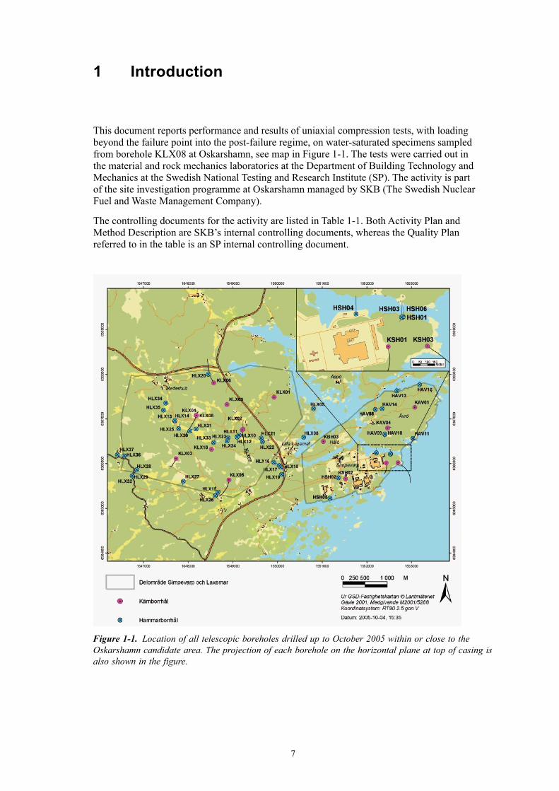
Two independent systems were used for the axial deformation measurement in order to obtain two comparative results. The first system (S1), see Figure �-2, comprises two aluminium rings attached on the specimen, placed at ¼ and ¾ of the specimen height. Two LVDTs mounted on the rings are used to measure the distance change between the rings on opposite sides of the specimen. As to the attachment, two rubber bands made of a thin rubber hose with 0.5 mm thickness are first mounted on the specimen right under where the two rings are to be posi-tioned. The rings are supplied with three adjustable spring-loaded screws, each with a rounded tip pointing on the specimen with 120 degrees division. The screw tips are thus pressing on the rubber band, when the rings are mounted. The second system (S2), see Figure �-�, consists of two aluminium plates clamped around the circular loading platens of steel on top and on bottom of the specimen. Two LVDTs, mounted on the plates, measure the distance change between these plates at opposite sides of the specimen at corresponding positions as for the first measurement system (S1).
The radial deformation was obtained by using a chain mounted around the specimen at mid-height, see Figures �-2 and �-�. The change of the chain-opening gap was measured by means of one LVDT and the circumferential, and thereby also the radial deformation could be obtained. See Appendix A.
The specimens were photographed with a 4.0 Mega pixel digital camera at highest resolution and the photographs were stored in a jpeg-format.
Figure 3-2. Left: Specimen with two rubber bands. Devices for local axial and circumferential deformation measurements attached on the specimen. Right: Rings and LVDTs for local axial deformation measurement.
1�
Figure 3-3. Left: Specimen inserted between the loading platens. The two separate axial deformation measurement devices can be seen: system (S1) that measures the local axial deformation (rings), and system (S2) that measures the deformation between the aluminium plates (total deformation). Right: Principal sketch showing the two systems used for the axial deformation measurements.

15
4 Execution
The water saturation and determination of the density of the wet specimens were made in accordance with the method description SKB MD 160.002 (SKB internal controlling docu-ment). This includes determination of density in accordance to ISRM /5/ and water saturation by SS EN 1�755 /6/. The uniaxial compression tests were carried out in compliance with the method description SKB MD 190.001 (SKB internal controlling document). The test method is based on ISRM suggested method /1/.
4.1 DescriptionofthespecimensThe rock type characterisation was made according to Stråhle /7/ using the SKB mapping system (Boremap). The identification marks, upper and lower sampling depth (Secup and Seclow) and the rock type according to Boremap are shown in Table 4-1.
4.2 SpecimenpreparationanddensitymeasurementThe temperature of the water was 19.0°C, which equals to a water density of 998.4 kg/m�, when the determination of the wet density of the rock specimens was carried out. Further, the specimens had been stored during 12 days in water when the density was determined.
An overview of the activities during the specimen preparation is shown in the step-by step description in Table 4-2.
Table4‑1. Specimenidentification,samplinglevel(boreholelength)androcktypeforallspecimens.
Identification Secup[m] Seclow[m] Rocktype
KLX08-113-1 586.63 586.80 Diorite/gabbroKLX08-113-2 586.80 586.97 Diorite/gabbro
KLX08-113-3 610.10 610.28 Diorite/gabbroKLX08-113-4 689.45 689.62 Diorite/gabbroKLX08-113-6 692.75 692.92 Diorite/gabbroKLX08-113-8 841.71 841.87 Diorite/gabbro
Table4‑2. Activitiesduringthespecimenpreparation.
Step Activity
1 The drill cores were marked where the specimens are to be taken.2 The specimens were cut to the specified length according to markings and the cutting surfaces
were grinded.3 The tolerances were checked: parallel and perpendicular end surfaces, smooth and straight
circumferential surface.4 The diameter and height were measured three times each. The respectively mean value
determines the dimensions that are reported.5 The specimens were then water saturated according to the method described in SKB MD 160.002
and were stored for minimum 7 days in water, whereupon the wet density was determined.

16
4.3 MechanicaltestingThe specimens had been stored 14–17 days in water when the uniaxial compression tests were carried out. The functionality of the testing system was checked before starting the tests. A check-list was filled in successively during the work in order to confirm that the different specified steps had been carried out. Moreover, comments were made upon observations made during the mechanical testing that are relevant for interpretation of the results. The check-list form is an SP internal quality document.
An overview of the activities during the mechanical testing is shown in the step-by step description in Table 4-�.
4.4 DatahandlingThe test results were exported as text files from the test software and stored in a file server on the SP computer network after each completed test. The main data processing, in which the elastic moduli were computed and the peak stress was determined, has been carried out using the program MATLAB /8/. Moreover, MATLAB was used to produce the diagrams shown in Section 5.1 and in Appendix B. The summary of results in Section 5.2 with tables containing mean value and standard deviation of the different parameters and diagrams were provided using MS Excel. MS Excel was also used for reporting data to the SICADA database.
Table4‑3. Activitiesduringthemechanicaltesting.
Step Activity
1 Digital photos were taken on each specimen before the mechanical testing.2 Devices for measuring axial and circumferential deformations were attached to the specimen.
3 The specimen was put in place and centred between the frame loading platens.4 The core on each LVDT was adjusted by means of a set screw to the right initial position. This was
done so that the optimal range of the LVDTs can be used for the deformation measurement.5 The frame piston was brought down into contact with the specimen with a force corresponding to
0.6 MPa axial stress.6 A load cycle with loading up to 5 MPa and unloading to 0.6 MPa was conducted in order to settle
possible contact gaps in the spherical seat in the piston and between the rock specimen and the loading platens.
7 The centring was checked again.8 The deformation measurement channels were zeroed in the test software.9 The loading was started and the initial loading rate was set to a radial strain rate of –0.025%/min.
The loading rate was increased after reaching the post-failure region. This was done in order to prevent the total time for the test to become too long.
10 The test was stopped either manually when the test had proceeded large enough to reveal the post-failure behaviour, or after severe cracking had occurred and it was judged that very little residual axial loading capacity was left in the specimen.
11 Digital photos were taken on each specimen after the mechanical testing.
17
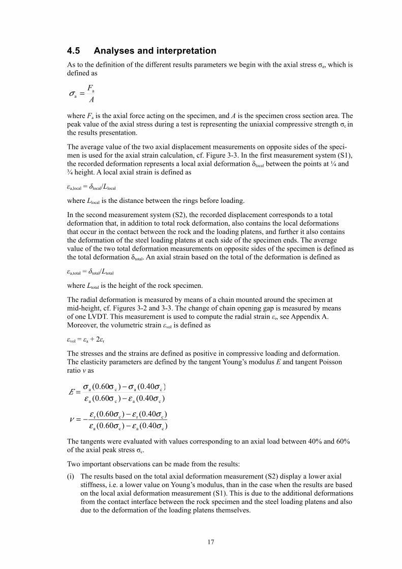
4.5 AnalysesandinterpretationAs to the definition of the different results parameters we begin with the axial stress σa, which is defined as
AFa
a =σ
where Fa is the axial force acting on the specimen, and A is the specimen cross section area. The peak value of the axial stress during a test is representing the uniaxial compressive strength σc in the results presentation.
The average value of the two axial displacement measurements on opposite sides of the speci-men is used for the axial strain calculation, cf. Figure �-�. In the first measurement system (S1), the recorded deformation represents a local axial deformation δlocal between the points at ¼ and ¾ height. A local axial strain is defined as
εa,local = δlocal/Llocal
where Llocal is the distance between the rings before loading.
In the second measurement system (S2), the recorded displacement corresponds to a total deformation that, in addition to total rock deformation, also contains the local deformations that occur in the contact between the rock and the loading platens, and further it also contains the deformation of the steel loading platens at each side of the specimen ends. The average value of the two total deformation measurements on opposite sides of the specimen is defined as the total deformation δtotal. An axial strain based on the total of the deformation is defined as
εa,total = δtotal/Ltotal
where Ltotal is the height of the rock specimen.
The radial deformation is measured by means of a chain mounted around the specimen at mid-height, cf. Figures �-2 and �-�. The change of chain opening gap is measured by means of one LVDT. This measurement is used to compute the radial strain εr, see Appendix A. Moreover, the volumetric strain εvol is defined as
εvol = εa + 2εr
The stresses and the strains are defined as positive in compressive loading and deformation. The elasticity parameters are defined by the tangent Young’s modulus E and tangent Poisson ratio ν as
)40.0()60.0()40.0()60.0(
caca
caca
σεσεσσσσ
−−
=E
)40.0()60.0()40.0()60.0(
caca
crcr
σεσεσεσεν
−−−=
The tangents were evaluated with values corresponding to an axial load between 40% and 60% of the axial peak stress σc.
Two important observations can be made from the results:
(i) The results based on the total axial deformation measurement (S2) display a lower axial stiffness, i.e. a lower value on Young’s modulus, than in the case when the results are based on the local axial deformation measurement (S1). This is due to the additional deformations from the contact interface between the rock specimen and the steel loading platens and also due to the deformation of the loading platens themselves.
18
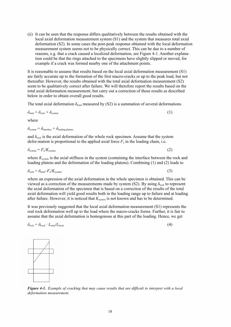
(ii) It can be seen that the response differs qualitatively between the results obtained with the local axial deformation measurement system (S1) and the system that measures total axial deformation (S2). In some cases the post-peak response obtained with the local deformation measurement system seems not to be physically correct. This can be due to a number of reasons, e.g. that a crack caused a localized deformation, see Figure 4-1. Another explana-tion could be that the rings attached to the specimens have slightly slipped or moved, for example if a crack was formed nearby one of the attachment points.
It is reasonable to assume that results based on the local axial deformation measurement (S1) are fairly accurate up to the formation of the first macro-cracks or up to the peak load, but not thereafter. However, the results obtained with the total axial deformation measurement (S2) seem to be qualitatively correct after failure. We will therefore report the results based on the total axial deformation measurement, but carry out a correction of those results as described below in order to obtain overall good results.
The total axial deformation δtotal measured by (S2) is a summation of several deformations
δtotal = δrock + δsystem (1)
where
δsystem = δinterface + δloading platens
and δrock is the axial deformation of the whole rock specimen. Assume that the system defor-mation is proportional to the applied axial force Fa in the loading chain, i.e.
δsystem = Fa/Ksystem (2)
where Ksystem is the axial stiffness in the system (containing the interface between the rock and loading platens and the deformation of the loading platens). Combining (1) and (2) leads to
δrock = δtotal–Fa/Ksystem (�)
where an expression of the axial deformation in the whole specimen is obtained. This can be viewed as a correction of the measurements made by system (S2). By using δrock to represent the axial deformation of the specimen that is based on a correction of the results of the total axial deformation will yield good results both in the loading range up to failure and at loading after failure. However, it is noticed that Ksystem is not known and has to be determined.
It was previously suggested that the local axial deformation measurement (S1) represents the real rock deformation well up to the load where the macro-cracks forms. Further, it is fair to assume that the axial deformation is homogenous at this part of the loading. Hence, we get
δrock = δlocal · Ltotal/Llocal (4)
Figure 4-1. Example of cracking that may cause results that are difficult to interpret with a local deformation measurement.

19
This yields representative values of the total rock deformation for the first part of the loading up to the point where macro-cracking is taking place. It is now possible to determine δsystem up to the threshold of macro-cracking by combining (1) and (4) which yields
δsystem = δtotal–δlocal · Ltotal/Llocal (5)
Finally, we need to compute Ksystem. By rewriting (2) we get
system
asystem δ
FK =
We will compute the system stiffness based on the results between 40% and 60% of the axial peak stress σc. This means that the Young’s modulus and the Poisson ratio will take the same values both when the data from the local axial deformation measurement (S1) and when the data from corrected total axial deformation are used. Thus, we have
)40.0()60.0()40.0()60.0(
csystemcsystem
cacasystem σδσδ
σσ−−= FFK (6)
The results based on the correction according to (�) and (6) are presented in Section 5.1, whereas the original measured unprocessed data are reported in Appendix B.
A closure of present micro-cracks will take place initially during axial loading. Development of new micro-cracks will start when the load is further increased and axial stress reaches the crack initiation stress σi. The crack growth at this stage is as stable as increased loading is required for further cracking. A transition from a development of micro-cracks to macro-cracks will occur when the axial load is further increased. At a certain stress level the crack growth becomes unstable. The stress level when this happens is denoted the crack damage stress σd, cf. /2/. In order to determine the stress levels, we look at the volumetric strain.
By subtracting the elastic volumetric strain evolε from the total volumetric strain, a volumetric
strain corresponding to the crack volume crvolε is obtained. This has been denoted calculated
crack volumetric strain in the literature, cf. /2, �/. We thus haveevolvol
crvol εεε −=
Assuming linear elasticity leads to
avolcrvol
21 σνεεE
−−=
where σr = 0 was used. Experimental investigations have shown that the crack initiation stress σi coincides with the onset of increase of the calculated crack volume, cf. /2, �/. The same investigations also indicate that the crack damage stress σd can be defined as the axial stress at which the total volume starts to increase, i.e. when a dilatant behaviour is observed.
4.6 NonconformitiesThe testing was conducted according to the method description with some deviations. The circumferential strains have been determined within a relative error of 1.5%, which is larger than what is specified in the ISRM-standard /1/. Further, double systems for measuring the axial deformation have been used, which is beyond the specifications in the method description. This was conducted as development of the test method specially aimed for high-strength brittle rock.
The activity plan was followed with no departures.

21
5 Results
The results of the individual specimens are presented in Section 5.1 and a summary of the results is given in Section 5.2. The reported parameters are based both on unprocessed raw data obtained from the testing and processed data and were reported to the SICADA database, where they are traceable by the activity plan number. These data together with the digital photographs of the individual specimens were handed over to SKB. The handling of the results follows SDP-508 (SKB internal controlling document) in general.
5.1 ResultsforeachindividualspecimenThe cracking is shown in pictures taken of the specimens and comments on observations made during the testing are reported. The elasticity parameters have been evaluated by using the results from the local axial deformation measurements. The data from the adjusted total axial deformation measurements, cf. Section 4.4, are shown in this section. Red rings are superposed on the graphs indicating every five minutes of the progress of testing.
Diagrams showing the data from both the local and the total axial deformation measurements, system (S1) and (S2) in Figure �-�, and the computed individual values of Ksystem used at the data corrections are shown in Appendix B. Diagrams displaying actual radial strain rates versus the test time are also presented in Appendix B. The results for the individual specimens are as follows:

22
SpecimenID:KLX08-11�-1
Before mechanical test After mechanical test
Diameter[mm]
Height[mm]
Density[kg/m3]
50.1 127.8 2,9�0
Comments: Spalling on one side of the specimen is observed.

2�
−1.4 −1.2 −1 −0.8 −0.6 −0.4 −0.20
50
100
150
200
250
300
350
400
Radial strain εr [%]
Axi
al s
tres
s σ a [M
Pa]
Specimen ID: KLX08−113−01
Youngs Modulus (E): 84.8 [GPa]
Poisson Ratio (ν): 0.386 [−]
Axial peak stress (σc): 215.2 [MPa]
0 0.2 0.4 0.6 0.8 1
Axial strain εa [%]
0 50 100 150 200 250 300 350 4000
0.05
0.1
0.15
0.2
0.25
Axial stress σa [MPa]
Vol
umet
ric s
trai
n ε vo
l [%]
−0.04
−0.035
−0.03
−0.025
−0.02
−0.015
−0.01
−0.005
0
0.005
0.01
Cra
ck v
olum
e st
rain
ε vol
cr [%
]

24
SpecimenID: KLX08-11�-2
Before mechanical test After mechanical test
Diameter[mm]
Height[mm]
Density[kg/m3]
50.1 127.8 2,9�0
Comments: Spalling on one side of the specimen is observed.

25
−1.4 −1.2 −1 −0.8 −0.6 −0.4 −0.20
50
100
150
200
250
300
350
400
Radial strain εr [%]
Axi
al s
tres
s σ a [M
Pa]
Specimen ID: KLX08−113−02
Youngs Modulus (E): 80.2 [GPa]
Poisson Ratio (ν): 0.363 [−]
Axial peak stress (σc): 216.4 [MPa]
0 0.2 0.4 0.6 0.8 1
Axial strain εa [%]
0 50 100 150 200 250 300 350 4000
0.05
0.1
0.15
0.2
0.25
Axial stress σa [MPa]
Vol
umet
ric s
trai
n ε vo
l [%]
−0.04
−0.035
−0.03
−0.025
−0.02
−0.015
−0.01
−0.005
0
0.005
0.01
Cra
ck v
olum
e st
rain
ε vol
cr [%
]

26
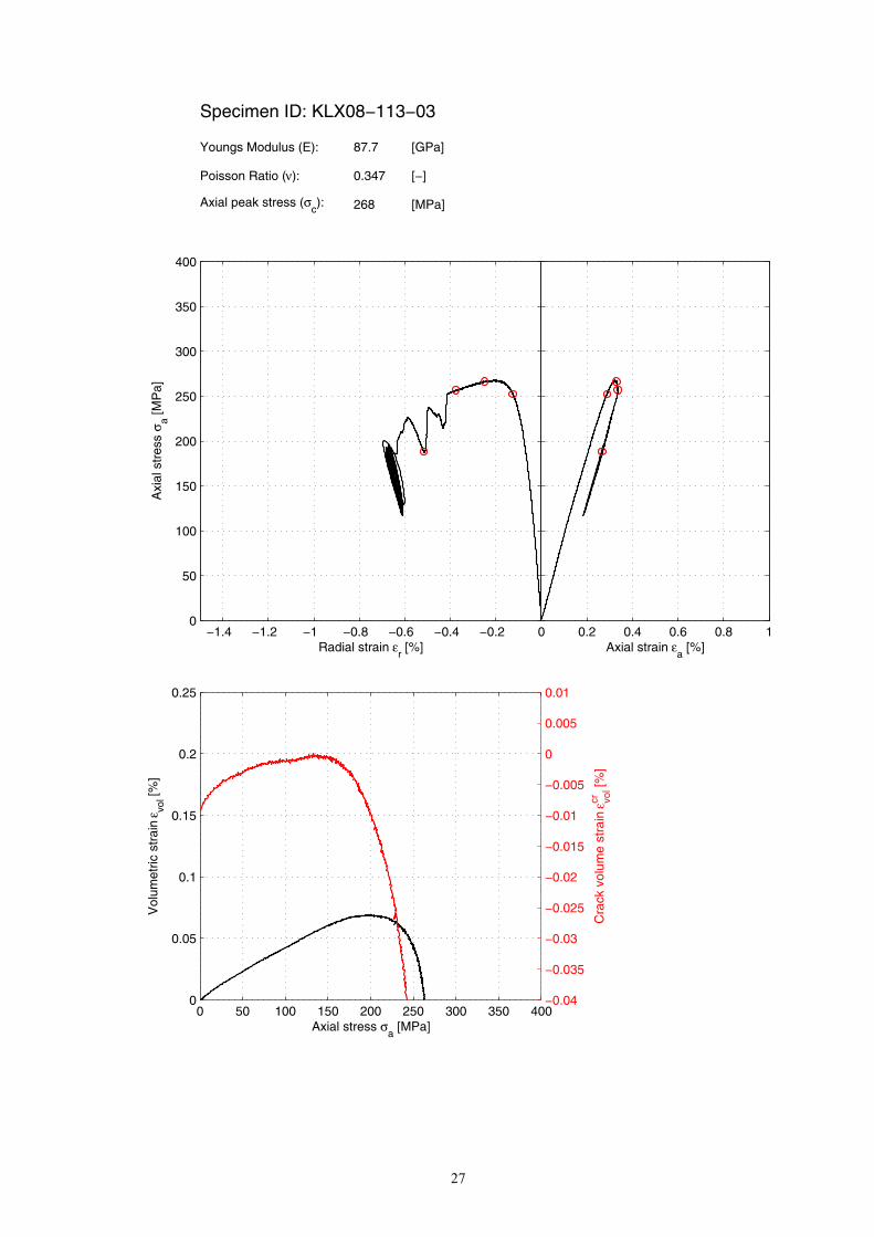
SpecimenID: KLX08-11�-�
Before mechanical test After mechanical test
Diameter[mm]
Height[mm]
Density[kg/m3]
50.1 127.8 2,890
Comments: Spalling on one side of the specimen is observed. The load started to oscillate when the radial strain had reached –0.7% and the test was stopped.
27
−1.4 −1.2 −1 −0.8 −0.6 −0.4 −0.20
50
100
150
200
250
300
350
400
Radial strain εr [%]
Axi
al s
tres
s σ a [M
Pa]
Specimen ID: KLX08−113−03
Youngs Modulus (E): 87.7 [GPa]
Poisson Ratio (ν): 0.347 [−]
Axial peak stress (σc): 268 [MPa]
0 0.2 0.4 0.6 0.8 1
Axial strain εa [%]
0 50 100 150 200 250 300 350 4000
0.05
0.1
0.15
0.2
0.25
Axial stress σa [MPa]
Vol
umet
ric s
trai
n ε vo
l [%]
−0.04
−0.035
−0.03
−0.025
−0.02
−0.015
−0.01
−0.005
0
0.005
0.01
Cra
ck v
olum
e st
rain
ε vol
cr [%
]

28
SpecimenID: KLX08-11�-4
Before mechanical test After mechanical test
Diameter[mm]
Height[mm]
Density[kg/m3]
49.9 127.8 2,870
Comments: Spalling on one side of the specimen is observed.

29
−1.4 −1.2 −1 −0.8 −0.6 −0.4 −0.20
50
100
150
200
250
300
350
400
Radial strain εr [%]
Axi
al s
tres
s σ a [M
Pa]
Specimen ID: KLX08−113−04
Youngs Modulus (E): 80.5 [GPa]
Poisson Ratio (ν): 0.321 [−]
Axial peak stress (σc): 219 [MPa]
0 0.2 0.4 0.6 0.8 1
Axial strain εa [%]
0 50 100 150 200 250 300 350 4000
0.05
0.1
0.15
0.2
0.25
Axial stress σa [MPa]
Vol
umet
ric s
trai
n ε vo
l [%]
−0.04
−0.035
−0.03
−0.025
−0.02
−0.015
−0.01
−0.005
0
0.005
0.01
Cra
ck v
olum
e st
rain
ε vol
cr [%
]

�0
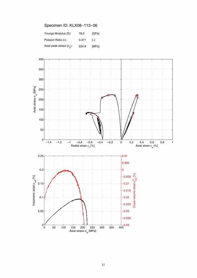
SpecimenID: KLX08-11�-6
Before mechanical test After mechanical test
Diameter[mm]
Height[mm]
Density[kg/m3]
49.9 128.1 2,870
Comments: Deep spalling is observed on one side of the specimen. The specimen fractured and the load started to oscillate when the radial strain had reached –0.5% and the test was stopped. The test was restarted one time.
�1
−1.4 −1.2 −1 −0.8 −0.6 −0.4 −0.20
50
100
150
200
250
300
350
400
Radial strain εr [%]
Axi
al s
tres
s σ a [M
Pa]
Specimen ID: KLX08−113−06
Youngs Modulus (E): 78.5 [GPa]
Poisson Ratio (ν): 0.311 [−]
Axial peak stress (σc): 224.8 [MPa]
0 0.2 0.4 0.6 0.8 1
Axial strain εa [%]
0 50 100 150 200 250 300 350 4000
0.05
0.1
0.15
0.2
0.25
Axial stress σa [MPa]
Vol
umet
ric s
trai
n ε vo
l [%]
−0.04
−0.035
−0.03
−0.025
−0.02
−0.015
−0.01
−0.005
0
0.005
0.01
Cra
ck v
olum
e st
rain
ε vol
cr [%
]

�2
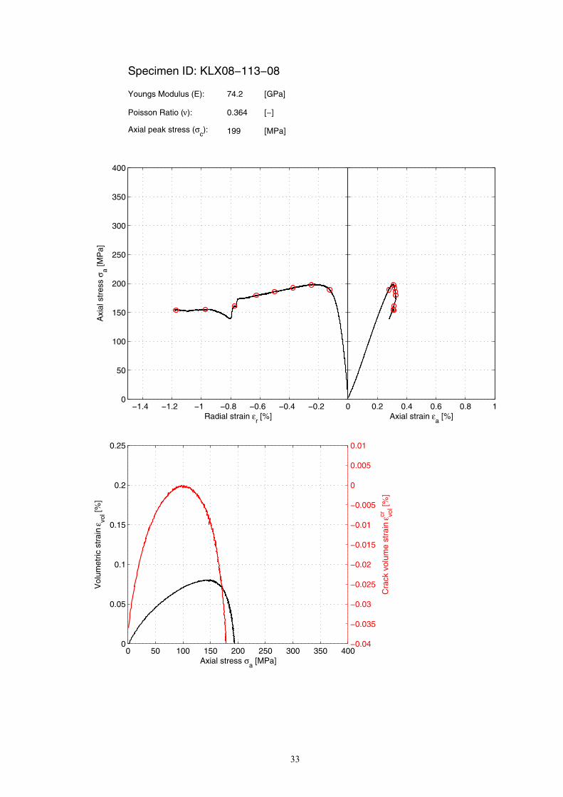
SpecimenID: KLX08-11�-8
Before mechanical test After mechanical test
Diameter[mm]
Height[mm]
Density[kg/m3]
50.0 127.8 2,8�0
Comments: Shallow spalling is observed on one side of the specimen.
��
−1.4 −1.2 −1 −0.8 −0.6 −0.4 −0.20
50
100
150
200
250
300
350
400
Radial strain εr [%]
Axi
al s
tres
s σ a [M
Pa]
Specimen ID: KLX08−113−08
Youngs Modulus (E): 74.2 [GPa]
Poisson Ratio (ν): 0.364 [−]
Axial peak stress (σc): 199 [MPa]
0 0.2 0.4 0.6 0.8 1
Axial strain εa [%]
0 50 100 150 200 250 300 350 4000
0.05
0.1
0.15
0.2
0.25
Axial stress σa [MPa]
Vol
umet
ric s
trai
n ε vo
l [%]
−0.04
−0.035
−0.03
−0.025
−0.02
−0.015
−0.01
−0.005
0
0.005
0.01
Cra
ck v
olum
e st
rain
ε vol
cr [%
]

�4
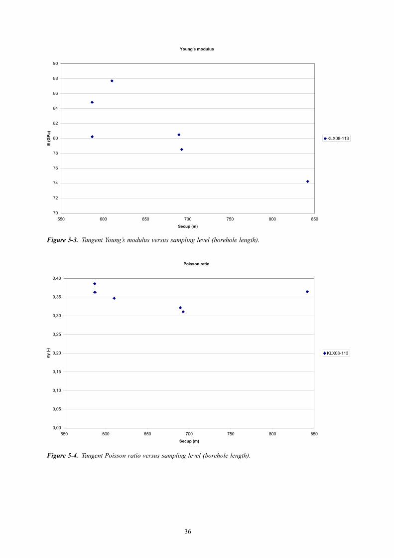
5.2 ResultsfortheentiretestseriesA summary of the test results is shown in Tables 5-1 and 5-2. The density, uniaxial compressive strength, the tangent Young’s modulus and the tangent Poisson ratio versus sampling level (borehole length) are shown in Figures 5-1 to 5-4.
Table5‑1. Summaryofresults.
Identification Density[kg/m3]
CompressiveStrength[MPa]
Young’smodulus[GPa]
Poissonratio[–]
Ksystem[GN/m]
KLX08-113-1 2,930 215.2 84.8 0.39 7.16KLX08-113-2 2,930 216.4 80.2 0.36 9.42
KLX08-113-3 2,890 268.0 87.7 0.35 6.98KLX08-113-4 2,870 219.0 80.5 0.32 11.71KLX08-113-6 2,870 224.8 78.5 0.31 13.93KLX08-113-8 2,830 199.0 74.2 0.36 13.40
Table5‑2. Calculatedmeanvaluesandstandarddeviation(Stddev)oftheresults.
Density[kg/m3]
CompressiveStrength[MPa]
Young’smodulus[GPa]
Poissonratio[–]
Mean value (586–610 m) 2,917 233.2 84.2 0.37Mean value (689–692 m) 2,870 221.9 79.5 0.32
Mean value (All levels) 2,887 223.7 81.0 0.35Std dev (586–610 m) 23.1 30.1 3.8 0.02Std dev (689–692 m) 0.0 4.1 1.4 0.01Std dev (All levels) 38.8 23.3 4.7 0.03

�5
Compressive strength
0
50
100
150
200
250
300
550 600 650 700 750 800 850
Secup (m)
Sigm
a C
(MPa
)
KLX08-113
Wet density
2800
2810
2820
2830
2840
2850
2860
2870
2880
2890
2900
2910
2920
2930
2940
2950
550 600 650 700 750 800 850
Secup (m)
Wet
den
sity
(kg/
m^3
)
KLX08-113
Figure 5-1. Density versus sampling level (borehole length).
Figure 5-2. Uniaxial compressive strength versus sampling level (borehole length).
�6
Figure 5-3. Tangent Young’s modulus versus sampling level (borehole length).
Figure 5-4. Tangent Poisson ratio versus sampling level (borehole length).
Young's modulus
70
72
74
76
78
80
82
84
86
88
90
550 600 650 700 750 800 850
Secup (m)
E (G
Pa)
KLX08-113
Poisson ratio
0,00
0,05
0,10
0,15
0,20
0,25
0,30
0,35
0,40
550 600 650 700 750 800 850
Secup (m)
ny (-
)
KLX08-113

�7
References
/1/ ISRM,1999. Draft ISRM suggested method for the complete stress-strain curve for intact rock in uniaxial compression. Int. J. Rock. Mech. Min. Sci. �6(�), pp. 279–289.
/2/ MartinCD,ChandlerNA,1994. The progressive fracture of Luc du Bonnet granite. Int. J. Rock. Mech. Min. Sci. & Geomech. Abstr. �1(6), pp. 64�–659.
/�/ EberhardtE,SteadD,StimpsonB,ReadRS,1998.Identifying crack initiation and propagation thresholds in brittle rock. Can. Geotech. J. �5, pp. 222–2��.
/4/ ASTM4543-01,2001. Standard practice for preparing rock core specimens and determining dimensional and shape tolerance.
/5/ ISRM,1979. Suggested Method for Determining Water Content, Porosity, Density, Absorption and Related Properties and Swelling and Slake-durability Index Properties. Int. J. Rock. Mech. Min. Sci. & Geomech. Abstr. 16(2), pp. 141–156.
/6/ SS-EN13755.Natural stone test methods – Determination of water absorption at atmospheric pressure.
/7/ StråhleA,2001. Definition och beskrivning av parametrar för geologisk, geofysisk och bergmekanisk kartering av berg, SKB-01-19. Svensk kärnbränslehantering AB. In Swedish.
/8/ MATLAB,2002.The Language of Technical computing. Version 6.5. MathWorks Inc.
�9
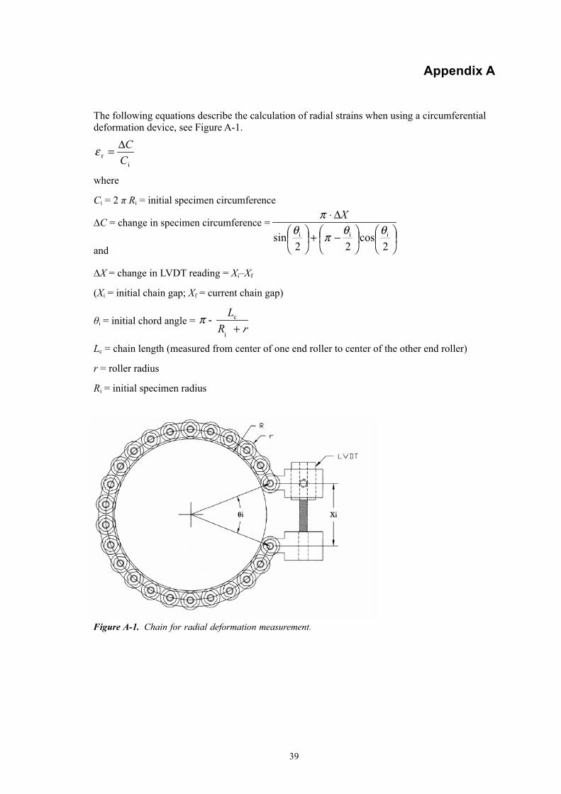
AppendixA
The following equations describe the calculation of radial strains when using a circumferential deformation device, see Figure A-1.
ir C
C∆=ε
where
Ci = 2 π Ri = initial specimen circumference
∆C = change in specimen circumference =
−+
∆⋅
2cos
22sin iii θθπθ
π X
and
∆X = change in LVDT reading = Xi–Xf
(Xi = initial chain gap; Xf = current chain gap)
θi = initial chord angle = π - rR
L+i
c
Lc = chain length (measured from center of one end roller to center of the other end roller)
r = roller radius
Ri = initial specimen radius
Figure A-1. Chain for radial deformation measurement.

41
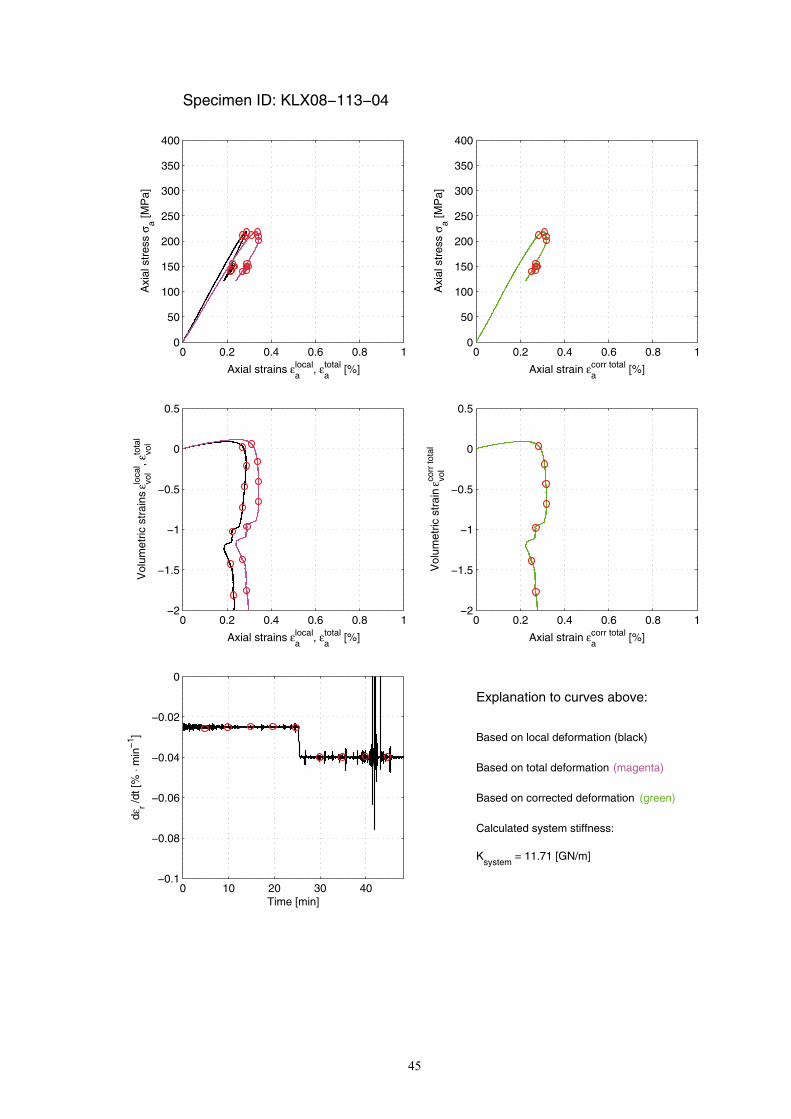
AppendixB
This Appendix contains results showing the unprocessed data and values on the computed system stiffness Ksystem that was used for the data processing, cf. Section 4.4. In addition graphs showing the volumetric strain εvol versus the axial strain εa and the actual radial strain rate dεr /dt versus time are also displayed.

42
0 0.2 0.4 0.6 0.8 10
50
100
150
200
250
300
350
400
Axial strains εlocala
, εtotala
[%]
Axi
al s
tres
s σ a [M
Pa]
Specimen ID: KLX08−113−01
0 0.2 0.4 0.6 0.8 10
50
100
150
200
250
300
350
400
Axial strain εcorr totala
[%]
Axi
al s
tres
s σ a [M
Pa]
0 0.2 0.4 0.6 0.8 1−2
−1.5
−1
−0.5
0
0.5
Axial strains εlocala
, εtotala
[%]
Vol
umet
ric s
trai
ns εlo
cal
vol
, εto
tal
vol
0 0.2 0.4 0.6 0.8 1−2
−1.5
−1
−0.5
0
0.5
Axial strain εcorr totala
[%]
Vol
umet
ric s
trai
n εco
rr to
tal
vol
0 10 20 30−0.1
−0.08
−0.06
−0.04
−0.02
0
Time [min]
dεr /d
t [%
⋅ m
in−
1 ]
Explanation to curves above:
Based on local deformation (black)
Based on total deformation (magenta)
Based on corrected deformation (green)
Calculated system stiffness:
Ksystem
= 7.16 [GN/m]

4�
0 0.2 0.4 0.6 0.8 10
50
100
150
200
250
300
350
400
Axial strains εlocala
, εtotala
[%]
Axi
al s
tres
s σ a [M
Pa]
Specimen ID: KLX08−113−02
0 0.2 0.4 0.6 0.8 10
50
100
150
200
250
300
350
400
Axial strain εcorr totala
[%]
Axi
al s
tres
s σ a [M
Pa]
0 0.2 0.4 0.6 0.8 1−2
−1.5
−1
−0.5
0
0.5
Axial strains εlocala
, εtotala
[%]
Vol
umet
ric s
trai
ns εlo
cal
vol
, εto
tal
vol
0 0.2 0.4 0.6 0.8 1−2
−1.5
−1
−0.5
0
0.5
Axial strain εcorr totala
[%]
Vol
umet
ric s
trai
n εco
rr to
tal
vol
0 10 20 30−0.1
−0.08
−0.06
−0.04
−0.02
0
Time [min]
dεr /d
t [%
⋅ m
in−
1 ]
Explanation to curves above:
Based on local deformation (black)
Based on total deformation (magenta)
Based on corrected deformation (green)
Calculated system stiffness:
Ksystem
= 9.42 [GN/m]

44
0 0.2 0.4 0.6 0.8 10
50
100
150
200
250
300
350
400
Axial strains εlocala
, εtotala
[%]
Axi
al s
tres
s σ a [M
Pa]
Specimen ID: KLX08−113−03
0 0.2 0.4 0.6 0.8 10
50
100
150
200
250
300
350
400
Axial strain εcorr totala
[%]
Axi
al s
tres
s σ a [M
Pa]
0 0.2 0.4 0.6 0.8 1−2
−1.5
−1
−0.5
0
0.5
Axial strains εlocala
, εtotala
[%]
Vol
umet
ric s
trai
ns εlo
cal
vol
, εto
tal
vol
0 0.2 0.4 0.6 0.8 1−2
−1.5
−1
−0.5
0
0.5
Axial strain εcorr totala
[%]
Vol
umet
ric s
trai
n εco
rr to
tal
vol
0 5 10 15 20−0.1
−0.08
−0.06
−0.04
−0.02
0
Time [min]
dεr /d
t [%
⋅ m
in−
1 ]
Explanation to curves above:
Based on local deformation (black)
Based on total deformation (magenta)
Based on corrected deformation (green)
Calculated system stiffness:
Ksystem
= 6.98 [GN/m]
45
0 0.2 0.4 0.6 0.8 10
50
100
150
200
250
300
350
400
Axial strains εlocala
, εtotala
[%]
Axi
al s
tres
s σ a [M
Pa]
Specimen ID: KLX08−113−04
0 0.2 0.4 0.6 0.8 10
50
100
150
200
250
300
350
400
Axial strain εcorr totala
[%]
Axi
al s
tres
s σ a [M
Pa]
0 0.2 0.4 0.6 0.8 1−2
−1.5
−1
−0.5
0
0.5
Axial strains εlocala
, εtotala
[%]
Vol
umet
ric s
trai
ns εlo
cal
vol
, εto
tal
vol
0 0.2 0.4 0.6 0.8 1−2
−1.5
−1
−0.5
0
0.5
Axial strain εcorr totala
[%]
Vol
umet
ric s
trai
n εco
rr to
tal
vol
0 10 20 30 40−0.1
−0.08
−0.06
−0.04
−0.02
0
Time [min]
dεr /d
t [%
⋅ m
in−
1 ]
Explanation to curves above:
Based on local deformation (black)
Based on total deformation (magenta)
Based on corrected deformation (green)
Calculated system stiffness:
Ksystem
= 11.71 [GN/m]

46
0 0.2 0.4 0.6 0.8 10
50
100
150
200
250
300
350
400
Axial strains εlocala
, εtotala
[%]
Axi
al s
tres
s σ a [M
Pa]
Specimen ID: KLX08−113−06
0 0.2 0.4 0.6 0.8 10
50
100
150
200
250
300
350
400
Axial strain εcorr totala
[%]
Axi
al s
tres
s σ a [M
Pa]
0 0.2 0.4 0.6 0.8 1−2
−1.5
−1
−0.5
0
0.5
Axial strains εlocala
, εtotala
[%]
Vol
umet
ric s
trai
ns εlo
cal
vol
, εto
tal
vol
0 0.2 0.4 0.6 0.8 1−2
−1.5
−1
−0.5
0
0.5
Axial strain εcorr totala
[%]
Vol
umet
ric s
trai
n εco
rr to
tal
vol
0 5 10 15 20 25−0.1
−0.08
−0.06
−0.04
−0.02
0
Time [min]
dεr /d
t [%
⋅ m
in−
1 ]
Explanation to curves above:
Based on local deformation (black)
Based on total deformation (magenta)
Based on corrected deformation (green)
Calculated system stiffness:
Ksystem
= 13.93 [GN/m]

47
0 0.2 0.4 0.6 0.8 10
50
100
150
200
250
300
350
400
Axial strains εlocala
, εtotala
[%]
Axi
al s
tres
s σ a [M
Pa]
Specimen ID: KLX08−113−08
0 0.2 0.4 0.6 0.8 10
50
100
150
200
250
300
350
400
Axial strain εcorr totala
[%]
Axi
al s
tres
s σ a [M
Pa]
0 0.2 0.4 0.6 0.8 1−2
−1.5
−1
−0.5
0
0.5
Axial strains εlocala
, εtotala
[%]
Vol
umet
ric s
trai
ns εlo
cal
vol
, εto
tal
vol
0 0.2 0.4 0.6 0.8 1−2
−1.5
−1
−0.5
0
0.5
Axial strain εcorr totala
[%]
Vol
umet
ric s
trai
n εco
rr to
tal
vol
0 10 20 30 40−0.1
−0.08
−0.06
−0.04
−0.02
0
Time [min]
dεr /d
t [%
⋅ m
in−
1 ]
Explanation to curves above:
Based on local deformation (black)
Based on total deformation (magenta)
Based on corrected deformation (green)
Calculated system stiffness:
Ksystem
= 13.4 [GN/m]