University of Bern

Master’s Thesis

Real-Time Anomaly Detection in Water DistributionNetworks using Spark Streaming

Stefan Nueschfrom Wabern

SupervisorsProf. Dr. Philippe Cudre-Mauroux

Djellel Eddine Difallah

Research GroupeXascale Infolab (Xi)

Departament of InformaticsUniversity of Fribourg

November 2014

Abstract

This thesis analyses the adequacy and the performance of the Apache SparkStreaming engine in the context of anomaly detection in water distributionnetworks (WDN). It builds on an already proposed scenario in which sensorsare extensively deployed in a WDN allowing for distributed, near-real-timeanomaly detection. For this purpose, it uses several variations of LISAstatistics and according statistical tests.In order to show that Spark Streaming is applicable to such a setting, al-gorithms computing these statistics in Spark Streaming were developed.Subsequently, the resulting prototype was tested in a simulated WDN setting.Finally, the performance of the different algorithms as well as the impact ofseveral network characteristics were measured.The results show that the calculation of LISA statistics can be achieved withreasonable performance by using Spark Streaming. Furthermore, they revealcertain characteristics and limitations of Spark Streaming.

Acknowledgements

First and foremost, I would like to thank Djellel Eddine Difallah andProfessor Philippe Cudre-Mauroux who supervised my work for their greatsupport throughout this thesis. Without their advice and ideas, this thesiswould not have been possible.I would also like to express my gratitude to the staff at eXascale Infolab1

for providing me access to their cluster and for supporting me in resolvingissues concerning this cluster.I would especially like to thank Bettina Stahli and Michael Hofer for theirsupport and their effort to correct this thesis. Their constructive criticismhelped me to greatly improve this thesis.

1http://www.exascale.info

ii

Contents

1 Introduction 1

2 Related Work 32.1 Local Indicators of Spatial Association . . . . . . . . . . . . . . . . . . 3

2.1.1 Spatial LISA . . . . . . . . . . . . . . . . . . . . . . . . . . . 42.1.2 Cluster / Outlier Type . . . . . . . . . . . . . . . . . . . . . . . 42.1.3 Temporal LISA . . . . . . . . . . . . . . . . . . . . . . . . . . 52.1.4 Statistical Significance - Monte Carlo Simulation . . . . . . . . 5

2.2 Apache Spark and Spark Streaming . . . . . . . . . . . . . . . . . . . . 72.2.1 Spark Architecture . . . . . . . . . . . . . . . . . . . . . . . . 72.2.2 Resilient Distributed Datasets . . . . . . . . . . . . . . . . . . 82.2.3 Dependencies and Scheduling . . . . . . . . . . . . . . . . . . 92.2.4 Spark Streaming . . . . . . . . . . . . . . . . . . . . . . . . . 10

2.2.4.1 Discretised Streams . . . . . . . . . . . . . . . . . . 112.2.4.2 Data Input . . . . . . . . . . . . . . . . . . . . . . . 12

2.2.5 Spark Streaming vs. Apache Storm . . . . . . . . . . . . . . . 122.3 Anomaly Detection in Water Distribution Networks . . . . . . . . . . . 13

3 Implementation 153.1 Architecture . . . . . . . . . . . . . . . . . . . . . . . . . . . . . . . . 15

3.1.1 Network Topology . . . . . . . . . . . . . . . . . . . . . . . . 163.1.2 Receiver . . . . . . . . . . . . . . . . . . . . . . . . . . . . . 183.1.3 Output Processing . . . . . . . . . . . . . . . . . . . . . . . . 19

3.2 Algorithms . . . . . . . . . . . . . . . . . . . . . . . . . . . . . . . . 193.2.1 Spatial LISA . . . . . . . . . . . . . . . . . . . . . . . . . . . 203.2.2 LISA with Temporal Association . . . . . . . . . . . . . . . . 223.2.3 Spatial Monte Carlo Simulation . . . . . . . . . . . . . . . . . 233.2.4 Temporal Monte Carlo Simulation . . . . . . . . . . . . . . . . 25

iii

4 Experiments 284.1 Setting . . . . . . . . . . . . . . . . . . . . . . . . . . . . . . . . . . . 28

4.1.1 Test Bed . . . . . . . . . . . . . . . . . . . . . . . . . . . . . 284.1.2 Topology . . . . . . . . . . . . . . . . . . . . . . . . . . . . . 294.1.3 Input / Output . . . . . . . . . . . . . . . . . . . . . . . . . . . 29

4.2 Spatial LISA Calculation . . . . . . . . . . . . . . . . . . . . . . . . . 294.3 LISA with Temporal Association . . . . . . . . . . . . . . . . . . . . . 344.4 Impact of Topology Density . . . . . . . . . . . . . . . . . . . . . . . 354.5 LISA with Monte Carlo Simulation . . . . . . . . . . . . . . . . . . . 374.6 LISA with Temporal Association and Monte Carlo Simulation . . . . . 40

5 Conclusion 425.1 Future Work . . . . . . . . . . . . . . . . . . . . . . . . . . . . . . . . 43

A Appendix 48A.1 Complete Source Code . . . . . . . . . . . . . . . . . . . . . . . . . . 48

iv

List of Figures

2.1 Spark Program Architecture (source: [21]) . . . . . . . . . . . . . . . . 82.2 Spark Dependencies (source: [21]) . . . . . . . . . . . . . . . . . . . . 92.3 Spark Scheduling Stages (source: [21]) . . . . . . . . . . . . . . . . . 102.4 DStream Processing Model (source: [23]) . . . . . . . . . . . . . . . . 11

3.1 Application Architecture Overview . . . . . . . . . . . . . . . . . . . . 163.2 Simple Topology Model (adapted from [18]) . . . . . . . . . . . . . . . 173.3 Legend . . . . . . . . . . . . . . . . . . . . . . . . . . . . . . . . . . 203.4 Spatial LISA Algorithm . . . . . . . . . . . . . . . . . . . . . . . . . . 213.5 Temporal LISA Algorithm . . . . . . . . . . . . . . . . . . . . . . . . 223.6 Spatial Monte Carlo Simulation - Naive Approach . . . . . . . . . . . . 233.7 Spatial Monte Carlo Simulation - Improved Approach . . . . . . . . . . 243.8 Temporal Monte Carlo Simulation . . . . . . . . . . . . . . . . . . . . 25

4.1 Single LISA Run for 1 and 16 Nodes . . . . . . . . . . . . . . . . . . . 304.2 Average Calculation Times . . . . . . . . . . . . . . . . . . . . . . . . 314.3 Sample CPU Usage in the Cluster . . . . . . . . . . . . . . . . . . . . 334.4 Sample Network Usage in the Cluster . . . . . . . . . . . . . . . . . . 334.5 Temporal LISA - Average Duration for Different K’s . . . . . . . . . . 354.6 Average Calculation Duration for Different Topology Types . . . . . . . 364.7 Scheduling Delays - Naive Approach . . . . . . . . . . . . . . . . . . . 374.8 Monte Carlo Simulation Performance - Naive Approach . . . . . . . . 384.9 Improved Monte Carlo Simulation Performance . . . . . . . . . . . . . 394.10 Temporal Monte Carlo - Algorithm Comparison . . . . . . . . . . . . . 40

v

List of Tables

4.1 Cluster Node Specifications (adapted from [20]) . . . . . . . . . . . . . 294.2 HDFS Save Duration per Number of Workers . . . . . . . . . . . . . . 314.3 Average Calculation Time per Number of Nodes and Cluster Workers . 324.4 Calculation Durations for Topology Types . . . . . . . . . . . . . . . . 364.5 Average Calculation Duration in Seconds . . . . . . . . . . . . . . . . 39

vi

List of listings

1 Sample Proximity Matrix File . . . . . . . . . . . . . . . . . . . . . . 182 Global Selection of Random Past Neighbour Values . . . . . . . . . . . 263 Local Selection of Random Past Neighbour Values . . . . . . . . . . . 26

vii

List of Acronyms

ADBMS Array Database Management System.

API Application Programming Interface.

CSR Complete Spatial Randomness.

DStream Discretised Stream.

HDFS Hadoop File System.

JVM Java Virtual Machine.

LISA Local Indicators of Spacial Association.

RDD Resilient Distributed Dataset.

WDN Water Distribution Network.

YARN Yet Another Resource Negotiator (Hadoop MapReduce 2.0).

viii

1Introduction

The ever growing availability of communication technology has lead to vast amountsof data being generated from the electronic monitoring of city infrastructure in today’surban areas. With emerging technologies capable of processing large amounts of data,efforts to leverage its value and to improve existing infrastructure have increased. Theresearch field pursuing these efforts is called Smarter Cities, and it covers numeroustypes of infrastructure including public and private transport, electrical networks andcommunication infrastructure.The present thesis deals with a particular type of infrastructure, namely water distribution.In traditional water distribution networks (WDNs), anomaly detection relies heavily onhuman labour, e.g. manual water quality sampling and reports by citizens. Automatedmonitoring usually only includes hydraulic parameters such as water pressure and flow,and covers only small parts of the WDN. Consequently, anomaly detection suffers fromhigh delays in traditional WDNs. Reacting to time sensitive issues such as theft andleakage is therefore difficult [13].D.E. Difallah, P. Cudre-Mauroux, and S.A McKenna proposed the use of Smarter Citiestechnologies as potential solution to these issues [13]. Their scenario envisages to deployaffordable sensors throughout the entire WDN which measure different characteristics,such as pressure, flow or water quality. These sensors send their measurements wirelesslyto intermediate computing stations (called base stations). Ultimately, the sensor data is

1

Chapter 1: Introduction

stored in an Array Database Management System (ADBMS). The goal of this implemen-tation is to detect anomalies in the network by using particular statistical metrics, whichare calculated on the base stations and stored along with the sensor data in the ADBMS.It has been shown that the architecture and the methods used in this approach are feasibleto detect anomalies in large scale WDN. Ongoing research in several related fields,however, has opened opportunities for improvements. In particular, stream processingsystems combinable with Big Data technologies have become available and are constantlyimproving. This thesis evaluates such a system in the context of the WDN outlinedabove.In detail, the goal of this thesis is to implement the statistical calculations proposedin [13], and to evaluate the performance of Spark Streaming in this scenario. For thispurpose, a prototype application is built to fit the architecture of the proposed systemwhose performance is then evaluated in various settings.

2

2Related Work

As mentioned in the previous chapter, the goal of this thesis is to implement statisticalcalculations with Spark Streaming and to evaluate the performance of the solution. Inthe following chapter, the theoretical background necessary for this purpose is explainedin three parts. In detail, the first part covers the statistical foundation for the algorithmimplementation. In the second part, the Big Data platform used for the implementationis explained. The third part briefly summarises the WDN application proposed in [13].

2.1 Local Indicators of Spatial Association

Spatial correlation statistics have been a part of geographical studies for many years.They provide a means for detecting clusters of similar values and outliers. Local indica-tors of spatial association (LISA) were first introduced for cluster and outlier detection ingeographical studies. They are based on observations of the same property at differentpoints in a two-dimensional space and express relationships between such observationsweighted by the spatial distance between them [12].Research has shown that LISA statistics may also be used as a means to detect localanomalies in WDNs [13]. For this purpose, they modelled the network topology as aproximity-matrix which contains, for each sensor, a row of distance values. These values

3

Chapter 2: Related Work

represent the length of the water pipe connection between two sensors (with length=0 iftwo sensors are not connected).For this thesis, a simplified version of this model is used, in which to each connectionbetween two nodes a weight of 1 is assigned. Nodes which are not directly interconnectedin the network are treated as non-related. Furthermore, in order to apply the originallytime stationary LISA indicators to a constant stream of sensor observations, the indicatorsare repeatedly calculated for observations recorded in distinct time intervals.

2.1.1 Spatial LISA

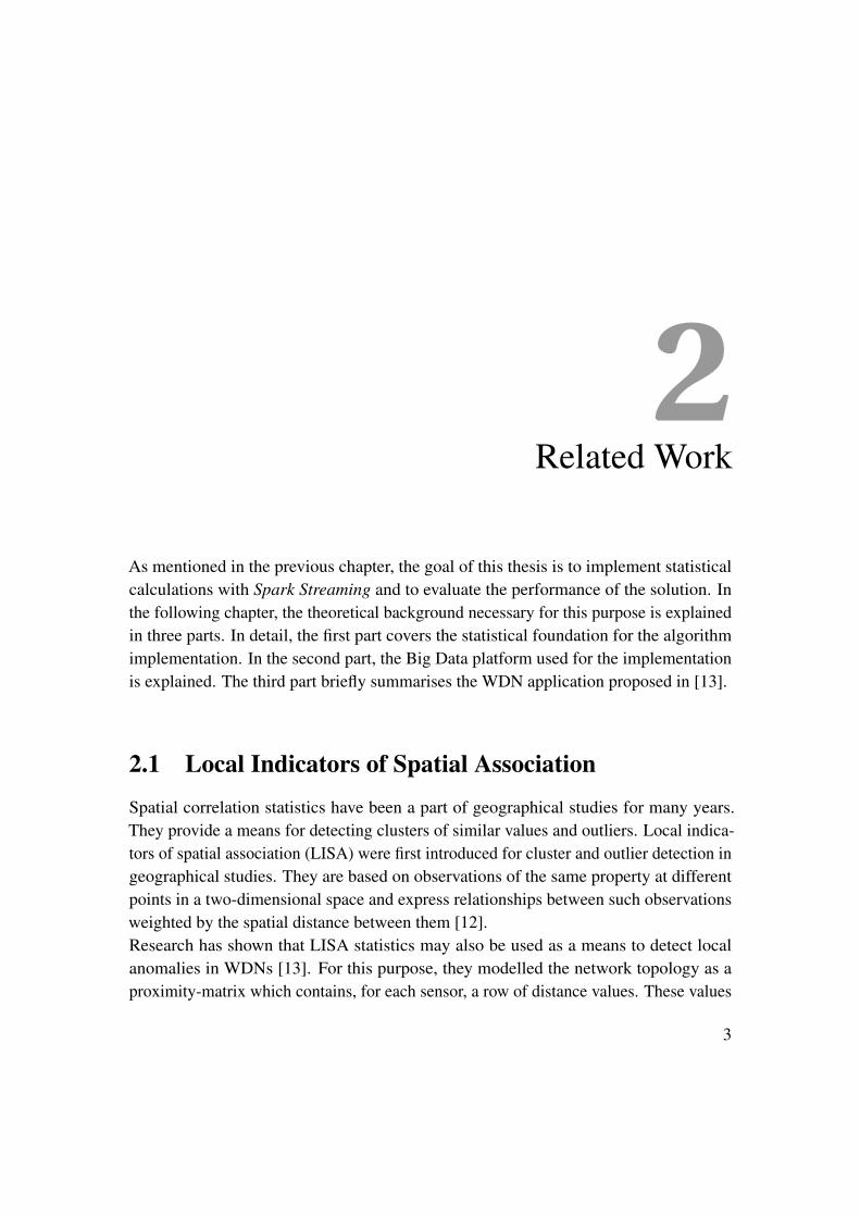
The spatial, time stationary LISA statistics used throughout this thesis is the local Moran’sI . It is defined in Equation 2.1, where va is the observed value at position a, N is thenumber of neighbouring (i.e. connected) sensors, vn is the measured value at neighbourn, m is the mean of all measured values and S is their standard deviation [14].

LISA(va) =

(va −mS

)[ N∑n=1

(1

N

)(vn −mS

)]

Equation 2.1: Spatial LISA

Spatial outliers are represented by negative values for LISA(va), while positivevalues indicate clusters. Furthermore, the ”magnitude [of the value] informs on the extentto which [original measurements] and neighbourhood values differ” [14].

2.1.2 Cluster / Outlier Type

While the local Moran’s I statistics provide a means to detect clusters and outliers, theyare not feasible to determine the cluster type. A strongly positive LISA(va) = I , forexample, identifies a local cluster. However, it cannot be used to determine if the clusteris a so-called hot-spot (high value amidst other high values, also called high-high or HH)or a cold-spot (low value amidst low values, also called low-low or LL). The same appliesto outliers (LH / HL) identified by negative values for I . While methods to determinetypes of clusters and outliers have been proposed (e.g. Getis-Ord Gi and G∗

i [12]), theyare not within the scope of this thesis [12] [14].

4

Chapter 2: Related Work

2.1.3 Temporal LISA

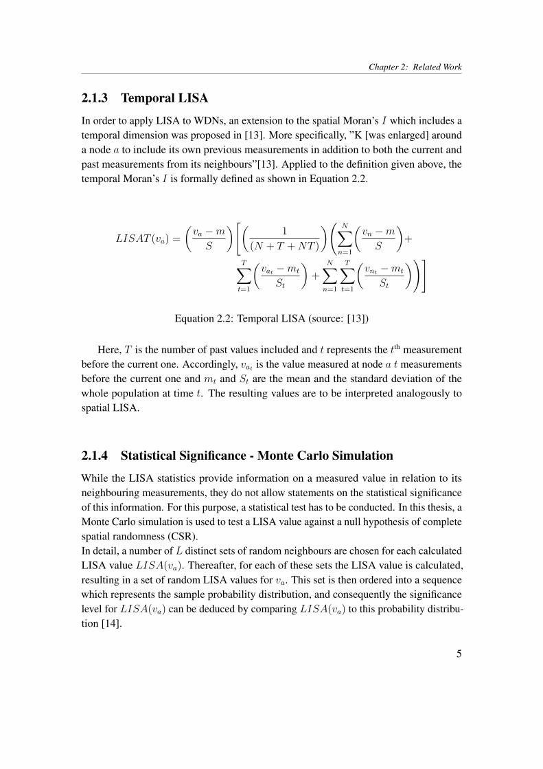
In order to apply LISA to WDNs, an extension to the spatial Moran’s I which includes atemporal dimension was proposed in [13]. More specifically, ”K [was enlarged] arounda node a to include its own previous measurements in addition to both the current andpast measurements from its neighbours”[13]. Applied to the definition given above, thetemporal Moran’s I is formally defined as shown in Equation 2.2.

LISAT (va) =

(va −mS

)[(1

(N + T +NT )

)( N∑n=1

(vn −mS

)+

T∑t=1

(vat −mt

St

)+

N∑n=1

T∑t=1

(vnt −mt

St

))]

Equation 2.2: Temporal LISA (source: [13])

Here, T is the number of past values included and t represents the tth measurementbefore the current one. Accordingly, vat is the value measured at node a t measurementsbefore the current one and mt and St are the mean and the standard deviation of thewhole population at time t. The resulting values are to be interpreted analogously tospatial LISA.

2.1.4 Statistical Significance - Monte Carlo Simulation

While the LISA statistics provide information on a measured value in relation to itsneighbouring measurements, they do not allow statements on the statistical significanceof this information. For this purpose, a statistical test has to be conducted. In this thesis, aMonte Carlo simulation is used to test a LISA value against a null hypothesis of completespatial randomness (CSR).In detail, a number of L distinct sets of random neighbours are chosen for each calculatedLISA value LISA(va). Thereafter, for each of these sets the LISA value is calculated,resulting in a set of random LISA values for va. This set is then ordered into a sequencewhich represents the sample probability distribution, and consequently the significancelevel for LISA(va) can be deduced by comparing LISA(va) to this probability distribu-tion [14].

5

Chapter 2: Related Work

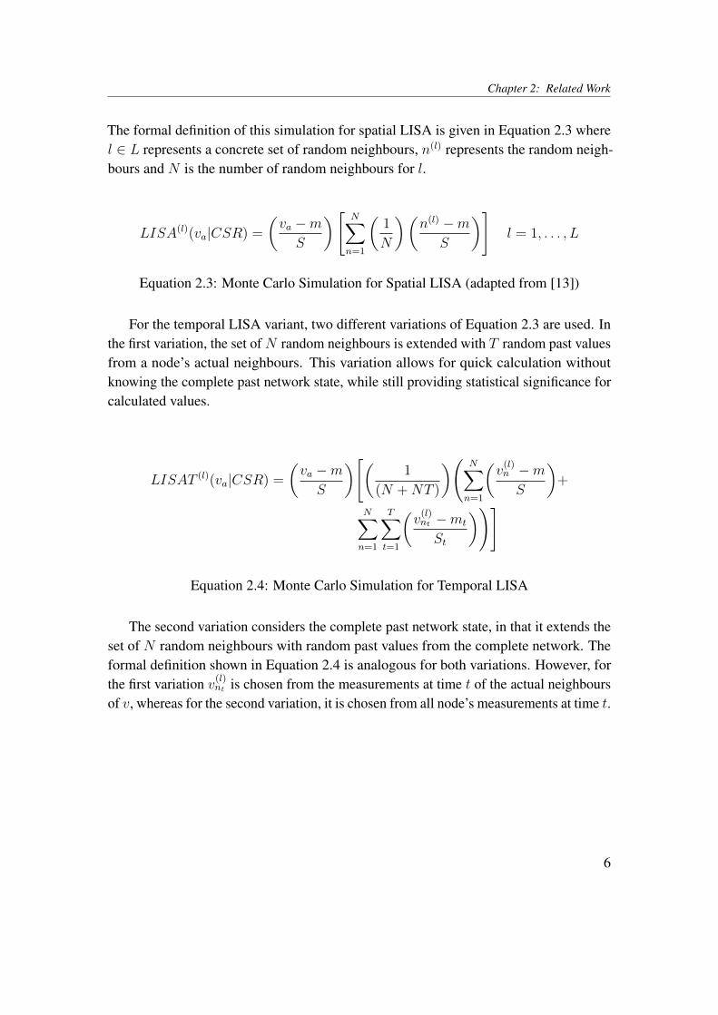
The formal definition of this simulation for spatial LISA is given in Equation 2.3 wherel ∈ L represents a concrete set of random neighbours, n(l) represents the random neigh-bours and N is the number of random neighbours for l.

LISA(l)(va|CSR) =(va −mS

)[ N∑n=1

(1

N

)(n(l) −m

S

)]l = 1, . . . , L

Equation 2.3: Monte Carlo Simulation for Spatial LISA (adapted from [13])

For the temporal LISA variant, two different variations of Equation 2.3 are used. Inthe first variation, the set of N random neighbours is extended with T random past valuesfrom a node’s actual neighbours. This variation allows for quick calculation withoutknowing the complete past network state, while still providing statistical significance forcalculated values.

LISAT (l)(va|CSR) =(va −mS

)[(1

(N +NT )

)( N∑n=1

(v(l)n −mS

)+

N∑n=1

T∑t=1

(v(l)nt −mt

St

))]

Equation 2.4: Monte Carlo Simulation for Temporal LISA

The second variation considers the complete past network state, in that it extends theset of N random neighbours with random past values from the complete network. Theformal definition shown in Equation 2.4 is analogous for both variations. However, forthe first variation v(l)nt is chosen from the measurements at time t of the actual neighboursof v, whereas for the second variation, it is chosen from all node’s measurements at time t.

6

Chapter 2: Related Work

2.2 Apache Spark and Spark Streaming

In recent years, the MapReduce programming model, and subsequently its various im-plementations and surrounding platforms (e.g. Apache Hadoop), have received muchattention both in science and in commerce. However, while Apache Hadoop provides aviable solution to many problems, recent work has shown various limitations with theprogramming model itself as well as with its field of application [16] [19] [17]. Morespecifically, applications which ”reuse a working set of data across multiple paralleloperations”[22] cannot be efficiently implemented by using MapReduce.To address this issue, researchers at the University of Berkeley created Spark, an open-source, in-memory cluster computing platform. This platform specifically targets ap-plications which run jobs iteratively or provide interactive query interfaces. Throughin-memory data processing Spark substantially enhances the performance of MapRe-duce-like applications without sacrificing scalability or fault-tolerance [22].The general-purpose data abstraction model introduced by Spark (cf. Section 2.2.2)furthermore allowed the platform to be expanded to suit different use cases. In particular,the need for a real-time data processing engine with a high-level interface was addressedby creating Spark Streaming. Building on the Spark platform, this component uses aninterval-based programming model to provide real-time processing capabilities whileassuring fault tolerance, consistency and integration with batch-processing [4].The Spark project was adopted as an Apache Incubator project in 2013 and was promotedto a top-level project in 2014. Consequently, the name of the platform was changed toApache Spark.

2.2.1 Spark Architecture

The Spark-platform is implemented in Scala and is hence run within the JVM. It can bedeployed as a standalone application on a cluster, as a client application of either ApacheHadoop 2+ (YARN) or Apache Mesos, or to a simulated cluster on a single machine(hereafter referred to as local master). In addition to a Scala API, interfaces in Java andPython are available. As the Scala API was used for the work presented in this thesis,the additional APIs are not discussed.

7

Chapter 2: Related Work

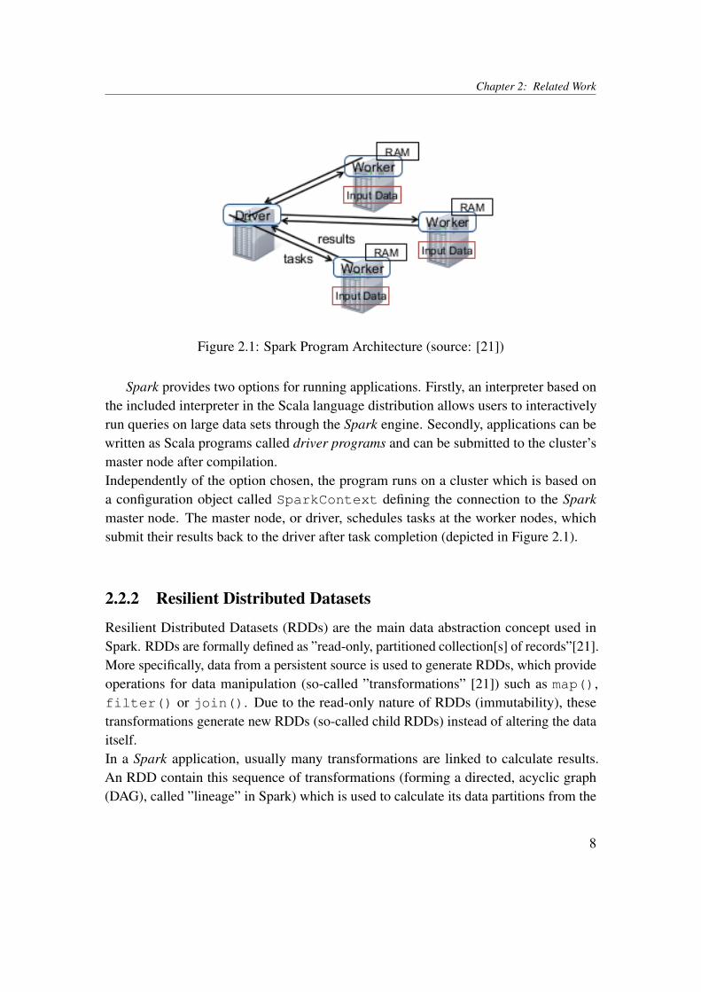
Figure 2.1: Spark Program Architecture (source: [21])

Spark provides two options for running applications. Firstly, an interpreter based onthe included interpreter in the Scala language distribution allows users to interactivelyrun queries on large data sets through the Spark engine. Secondly, applications can bewritten as Scala programs called driver programs and can be submitted to the cluster’smaster node after compilation.Independently of the option chosen, the program runs on a cluster which is based ona configuration object called SparkContext defining the connection to the Sparkmaster node. The master node, or driver, schedules tasks at the worker nodes, whichsubmit their results back to the driver after task completion (depicted in Figure 2.1).

2.2.2 Resilient Distributed Datasets

Resilient Distributed Datasets (RDDs) are the main data abstraction concept used inSpark. RDDs are formally defined as ”read-only, partitioned collection[s] of records”[21].More specifically, data from a persistent source is used to generate RDDs, which provideoperations for data manipulation (so-called ”transformations” [21]) such as map(),filter() or join(). Due to the read-only nature of RDDs (immutability), thesetransformations generate new RDDs (so-called child RDDs) instead of altering the dataitself.In a Spark application, usually many transformations are linked to calculate results.An RDD contain this sequence of transformations (forming a directed, acyclic graph(DAG), called ”lineage” in Spark) which is used to calculate its data partitions from the

8

Chapter 2: Related Work

original data. The lineage graph is used to regenerate an RDD after a failure, ensuringfault-tolerance within an application. In addition to the lineage, RDDs contain meta datasuch as information on the location of their data partitions.Moreover, RDDs also provide operations called ”actions” which yield one or several val-ues as a result. These actions include count(), foreach() and saveAsTextFile(),among others. Commonly, these actions are used to store data either on a file system, orin an arbitrary destination using foreach() [21].

2.2.3 Dependencies and Scheduling

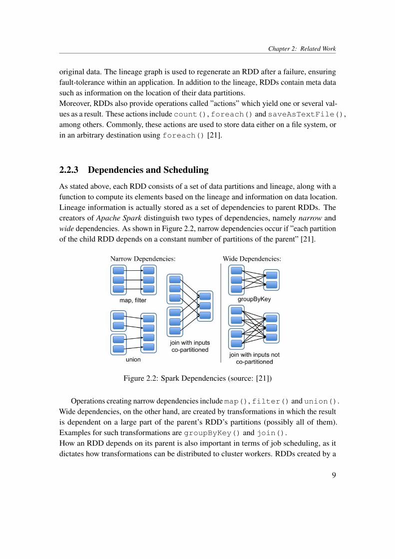
As stated above, each RDD consists of a set of data partitions and lineage, along with afunction to compute its elements based on the lineage and information on data location.Lineage information is actually stored as a set of dependencies to parent RDDs. Thecreators of Apache Spark distinguish two types of dependencies, namely narrow andwide dependencies. As shown in Figure 2.2, narrow dependencies occur if ”each partitionof the child RDD depends on a constant number of partitions of the parent” [21].

Figure 2.2: Spark Dependencies (source: [21])

Operations creating narrow dependencies include map(), filter() and union().Wide dependencies, on the other hand, are created by transformations in which the resultis dependent on a large part of the parent’s RDD’s partitions (possibly all of them).Examples for such transformations are groupByKey() and join().How an RDD depends on its parent is also important in terms of job scheduling, as itdictates how transformations can be distributed to cluster workers. RDDs created by a

9

Chapter 2: Related Work

transformation with narrow dependencies permit that each partition can be computed in-dependently of other partitions on a cluster worker. In case of wide dependencies, on theother hand, ”data from all parent partitions [is required] to be available and to be shuffledacross the nodes using a MapReduce-like operation” [21]. The scheduler used by ApacheSpark considers this information as depicted in Figure 2.3. It groups transformations intostages, each of which contains as many transformations with narrow dependencies aspossible. Stages are delimited by transformation with wide dependencies. This allows todistribute easily parallelisable task (i.e. narrow dependencies) efficiently [21].

Figure 2.3: Spark Scheduling Stages (source: [21])

2.2.4 Spark Streaming

As an extension to the Apache Spark batch processing platform, the creators of ApacheSpark implemented a stream processing engine called Spark Streaming. For processingthe input streams Spark Streaming uses an approach which differs from many existingstreaming engines (such as Storm or Samza). While these systems are event based, andhence process each record in real time, Spark Streaming uses a ”micro-batch” [15] [7].More specifically, Spark Streaming captures input from a stream for a pre-defined interval.At the end of the interval, it creates a batch upon which data manipulation operations areperformed. Each batch is stored as a set of RDDs, which allows the data to be processedby using the Apache Spark engine. An API, called Discretised Stream (DStream), formanipulating data on such streams of RDDs is provided by Spark Streaming.

10

Chapter 2: Related Work

2.2.4.1 Discretised Streams

Analogously to RDDs in Apache Spark, Spark Streaming programs define transforma-tions and actions on DStreams to manipulate and store data read from an input stream.Several connectors to input sources are provided by the DStream API, along with severaltypes of transformations and output actions.A distinction can be drawn between two types of transformations available on DStreams.There are transformation such as map() or filter()which can be applies to DStreamsof any type, whereas some transformations can only be applied to DStreams which con-tain key-value tuples. join(), groupByKey() and reduceByKey() are examplesof such transformations.All transformations described above are stateless, meaning that for each batch inter-val only the data collected in this interval is considered. However, Spark Streamingalso provides several ways of making transformations stateful. Firstly, ”windowing” aDStream creates a sliding window over several batch intervals. For example, callingwindow(Seconds(5)) on a DStream in a job with a batch duration of one secondwill yield a DStream containing, at each batch interval, input data of the last five seconds.Secondly, data can also be aggregated over time by using either more specialised formsof windowing such as reduceByWindow() or the updateStateByKey() trans-formation [23].

Figure 2.4: DStream Processing Model (source: [23])

11

Chapter 2: Related Work

Figure 2.4 depicts the programming model described above. In particular, two subse-quent batches of the same program are shown. At t = 1, the input dataset in transformedusing stateless transformations. The resulting dataset is included in the transformationsat t = 2 by using a stateful transformation.

2.2.4.2 Data Input

As stated above, there are several connectors for input streams already included in SparkStreaming, namely connectors for Apache Kafka, Apache Flume, Twitter, ZeroMQ, Ama-zon Kinesis and MQTT. Furthermore, connectors for reading from file systems and forlistening on a socket are included. However, the API of Spark Streaming also allows forcreating custom input stream sources, called receivers.The receiver API provides methods to repeatedly push data to a Spark Streaming applica-tion. Spark Streaming collects the data and processes it according to the driver applicationat each batch interval. One or multiple instances of such receivers can be registered withan application, each of which provides a separate DStream within the driver program. Atapplication start-up, Spark Streaming creates the instances and registers them as tasks atdifferent cluster nodes [3].

2.2.5 Spark Streaming vs. Apache Storm

Stream processing systems which target Big Data use cases have become more and morepopular in recent years. Most notably, Apache Storm has gained much attention as itgreatly simplifies both configuration and application programming compared to earlierreal-time stream computation approaches [9]. In an earlier master thesis, Simpal Kumarused Apache Storm to compute LISA statistics in the context of WDN [18]. In orderto differentiate this thesis from the work presented in [18], the following section givesa brief overview of the similarities and differences between Apache Storm and SparkStreaming .In terms of application management, the two systems are similar. In particular, bothsystems use a single application master node, called Nimbus in Apache Storm and drivernode in Spark Streaming. In addition, in both systems cluster workers receive parts of theapplication code to run. However, in Apache Storm state management and coordinationbetween the Nimbus and the worker program instances (called Supervisors) is handledby Zookeeper. Hence, both the Nimbus and the Supervisors are stateless while the driver

12

Chapter 2: Related Work

node handles state in Spark Streaming [10].In contrast to the cluster management, the stream processing is handled differently in thetwo systems. Apache Storm processes tuples of input values in an event based fashion,so that each arriving input value is processed as it enters the program, whereas SparkStreaming uses a micro-batch approach as described in Section 2.2.4.The programming model offered by Apache Storm is comparable to some extent to theone offered by Spark Streaming. Programs written for Apache Storm define Topologieswhich consist of input sources (Spouts) and operations (Bolts), and express a graphof operations which is traversed by each tuple of input values. Spouts are similar toreceivers in Spark Streaming and Bolts correspond to DStream operations. However,the way in which operation parallelism is achieved is different in the two systems. InSpark Streaming, the master node distributes Scala closures to workers, which processdata simultaneously (data parallelism [6]). Apache Storm, on the other hand, createstasks from Bolts and distributes these on the cluster to run them simultaneously (taskparallelism [11]) [8] [5].Consequently, aggregation operations cannot be done as simple calls in Apache Storm.Instead, Bolts have to be registered with so-called field groupings. Thereby, tuples withequal values in one field are distributed to the same worker task which in turn enablesaggregation operations.In conclusion, while Spark Streaming and Apache Storm offer similar capabilities forstream processing, their architectures differ considerably. Most notably, Apache Stormuses a record-at-a-time processing model, whereas Spark Streaming processes streamdata as micro-batches, which leads to different programming models.

2.3 Anomaly Detection in Water Distribution Networks

As already mentioned, the fundamental framework of this thesis is a WDN scenariodescribed in [13]. This scenario covers a complete architecture for anomaly detectionin the context of WDN, including a multi-layered hardware architecture as well as theaccording software components. It also shows how LISA statistics can be applied in thecontext of a continuous-time setting.The base layer of the hardware architecture consists of sensors deployed at the networknodes, i.e. ”pipe junctions and network end points where water is extracted for consump-tion” [13]. These sensor are simple electronic devices designed for durability and energyefficiency and are consequently limited in terms of functionality. More specifically, they

13

Chapter 2: Related Work

only need to measure particular characteristics of the WDN and to periodically transmitthese measurements to intermediate computing stations.These so-called base stations serve several purposes. Apart from collecting sensor mea-surements, they calculate local LISA statistics. Furthermore, they are interconnectedand form an overlay network in which measurements and detected anomalies are shared.Finally, an ADBMS stores all sensor measurements and anomalies, and provides meansfor more complex analytic operations. In particular, LISA statistics can be calculatedglobally by using data from the complete network [13].

14

3Implementation

To evaluate if and how the original scenario described in [13] can be applied to SparkStreaming, several prototypes for different algorithms have been developed in the courseof this thesis. This chapter covers the general architecture of these prototypes as well assome abstractions and simplifications made from the original implementation. Further-more, the core algorithms of the implementation, which calculate the statistical measuresdescribed in Section 2.1, are explained in detail.

3.1 Architecture

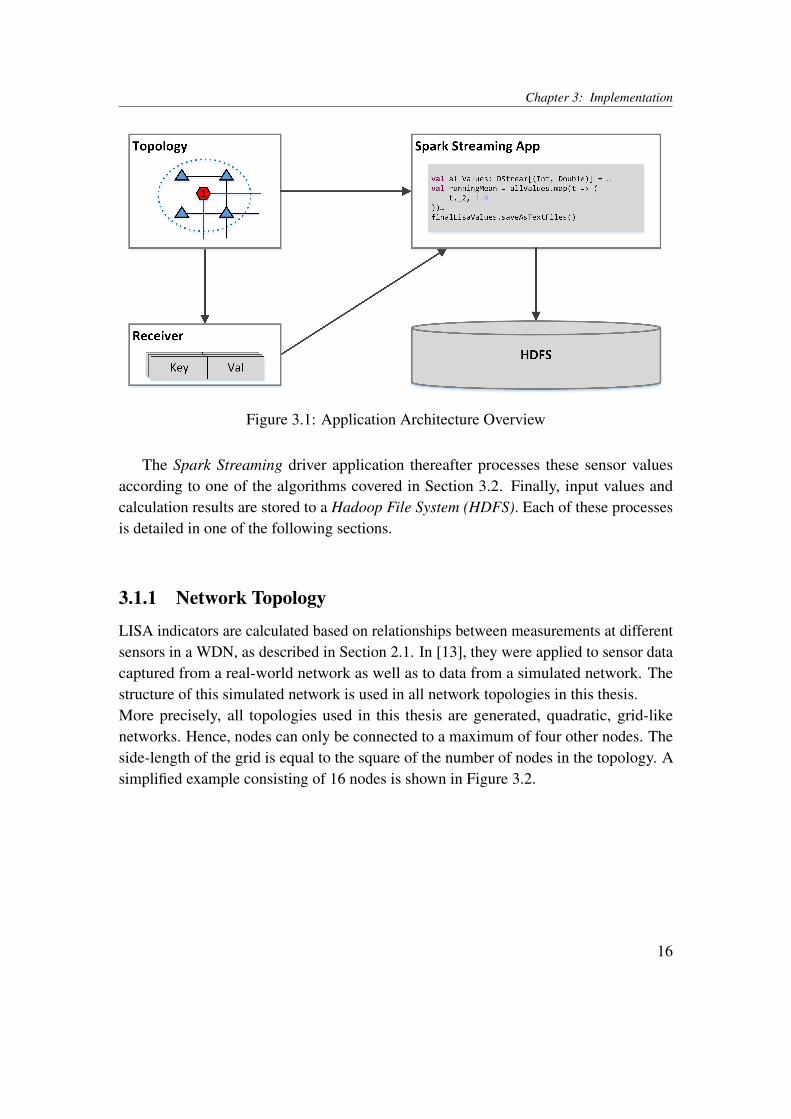
Figure 3.1 shows an overview of the application architecture used in all scenarios whichare explained in the following. Based on information on a simulated WDN topologysensor values (key-value pairs in the figure) are generated by a Spark Streaming receiver.

15

Chapter 3: Implementation

Figure 3.1: Application Architecture Overview

The Spark Streaming driver application thereafter processes these sensor valuesaccording to one of the algorithms covered in Section 3.2. Finally, input values andcalculation results are stored to a Hadoop File System (HDFS). Each of these processesis detailed in one of the following sections.

3.1.1 Network Topology

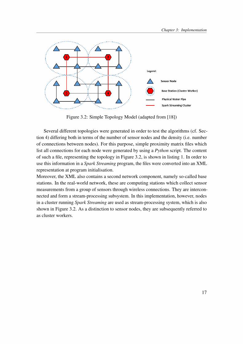
LISA indicators are calculated based on relationships between measurements at differentsensors in a WDN, as described in Section 2.1. In [13], they were applied to sensor datacaptured from a real-world network as well as to data from a simulated network. Thestructure of this simulated network is used in all network topologies in this thesis.More precisely, all topologies used in this thesis are generated, quadratic, grid-likenetworks. Hence, nodes can only be connected to a maximum of four other nodes. Theside-length of the grid is equal to the square of the number of nodes in the topology. Asimplified example consisting of 16 nodes is shown in Figure 3.2.

16

Chapter 3: Implementation

Figure 3.2: Simple Topology Model (adapted from [18])

Several different topologies were generated in order to test the algorithms (cf. Sec-tion 4) differing both in terms of the number of sensor nodes and the density (i.e. numberof connections between nodes). For this purpose, simple proximity matrix files whichlist all connections for each node were generated by using a Python script. The contentof such a file, representing the topology in Figure 3.2, is shown in listing 1. In order touse this information in a Spark Streaming program, the files were converted into an XMLrepresentation at program initialisation.Moreover, the XML also contains a second network component, namely so-called basestations. In the real-world network, these are computing stations which collect sensormeasurements from a group of sensors through wireless connections. They are intercon-nected and form a stream-processing subsystem. In this implementation, however, nodesin a cluster running Spark Streaming are used as stream-processing system, which is alsoshown in Figure 3.2. As a distinction to sensor nodes, they are subsequently referred toas cluster workers.

17

Chapter 3: Implementation

1 01000000000000002 10000100000000003 00010000000000004 00100001000000005 00000100000000006 01001010010000007 00000101000000008 00010010000000009 0000000000001000

10 000001000010000011 000000000101001012 000000000010000113 000000001000010014 000000000000101015 000000000010010016 0000000000010000

Listing 1: Sample Proximity Matrix File

3.1.2 Receiver

As stated above, all network topologies used in this thesis are artificial. As no actualsensor data was available for the Spark Streaming program the data needed to be simu-lated. In order to mimic the behaviour of sensors and base stations in a real-world WDN,simulated values for separate parts of the network are collected at each cluster worker(as shown with dotted blue areas in Figure 3.2).As described in Section 2.2.4.2, Spark Streaming provides an API for writing custominput sources, called receivers. While this receiver API is quite well suited to pushsimulated sensor data into a Spark Streaming application, it is not possible to controlat which cluster worker a receiver instance will be registered. As they are registered asSpark tasks, it is even possible that multiple receivers may be assigned to a single worker.This behaviour may have negative impact on the performance of an application, as taskslots are occupied by receivers for the whole run time of an application.Consequently, recreating the exact application structure described in [13] using SparkStreaming was not feasible. Instead, a single receiver instance for simulated sensorvalues was used for all algorithms. There are two different variations of the receiverimplementation for spatial and temporal LISA calculations. In case of spatial LISA, thereceiver emits tuples containing an integer as sensor node key and a simulated sensorvalue. In case of temporal LISA, instead of a single value, an array of length k + 1

containing one new value as well as the k last values is emitted. Here, k is a parameterconfigurable for each application run.

18

Chapter 3: Implementation

In the real-world topology, a sensor measures a number of different metrics, such aswater quality and pressure. As the presented implementation focuses on the calculationsand the performance of Spark Streaming rather than on the one-to-one applicability tothe real-world scenario, only values for a single artificial metric are emitted by eachsensor. More specifically, for each sensor node random values distributed accordingto a Gaussian function with Mean 0.0 and Standard Deviation 1.0 are generated at thereceiver.The rate at which these values are pushed into the application has been adapted to thecharacteristics of Spark Streaming. To ensure correctness of the LISA calculations,exactly one value per sensor and batch duration is generated. Consequently, the sensorrate is aligned with the batch duration of an application run. This issue is discussed infurther detail in Section 4.

3.1.3 Output Processing

The DStream API provided by Spark Streaming offers a simple output function whichis used for all output, namely saveAsTextFile(). For the algorithm describedsubsequently, this function is used to store both input values and final results to a HDFSlocation. Several Python scripts are used to validate the calculated results, and to parsethe log files written by Spark Streaming for performance evaluation.

3.2 Algorithms

The following section details the implementation of the various LISA and Monte Carloalgorithms with Spark Streaming. Important parts of all algorithms are depicted asgraphs, which consist of the elements shown in the legend in Figure 3.3. All graphs showsequences of operations (depicted as connectors) on DStreams (blocks).

19

Chapter 3: Implementation

Figure 3.3: Legend

3.2.1 Spatial LISA

The input of the LISA algorithm consists of key-value pairs in the form (key(a), vala)

for each sensor a emitted by the custom receiver described above. As explained inSection 2.1, all values need to be standardised by using the form (V alue−Mean)

StandardDeviation. Conse-

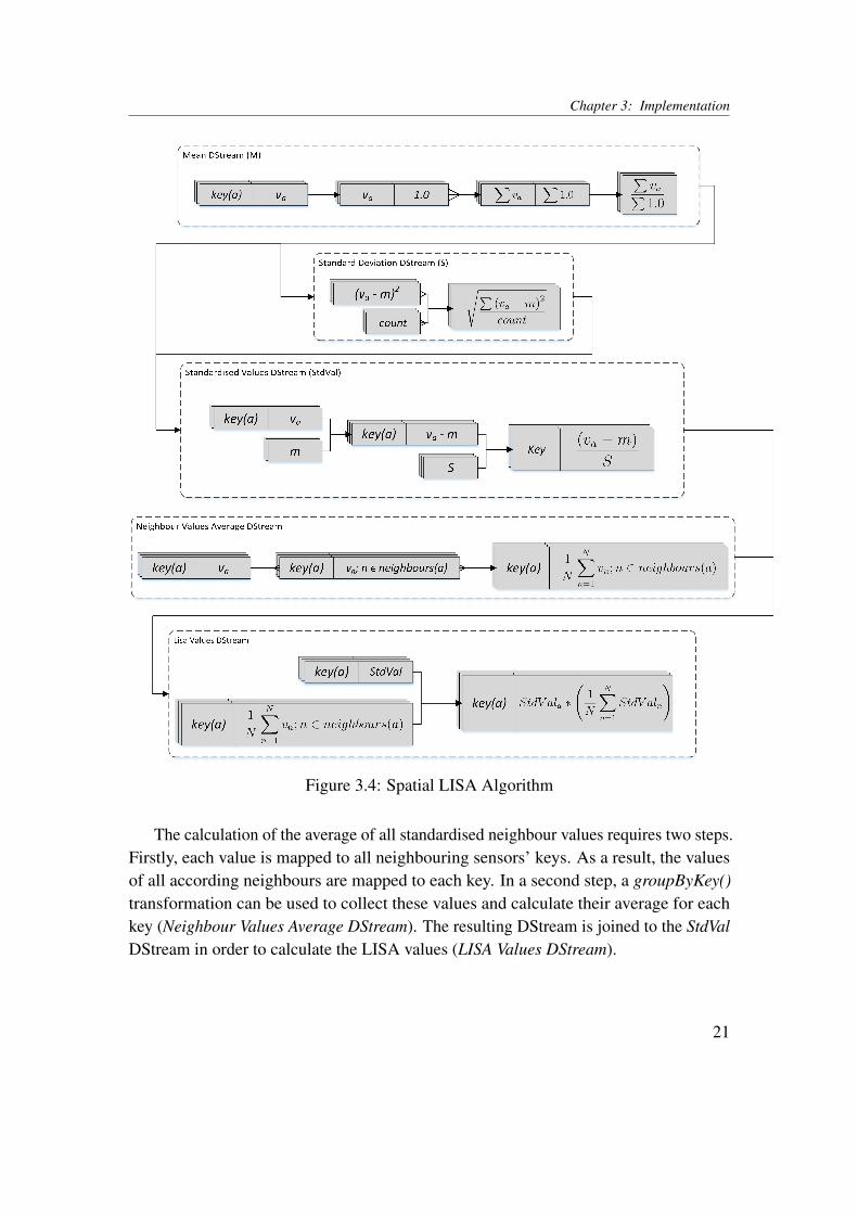
quently, as shown in Figure 3.4, calculating both the mean and the standard deviation arethe first steps in the algorithm, where the resulting DStream (Mean DStream (M)) fromthe calculation of the mean value is used to calculate the standard deviation (StandardDeviation DStream (S)). In a next step the standardised values (StdVal) are calculated bymapping M as well as S to each value of the initial DStream by using a simple map()transformation.

20

Chapter 3: Implementation

Figure 3.4: Spatial LISA Algorithm

The calculation of the average of all standardised neighbour values requires two steps.Firstly, each value is mapped to all neighbouring sensors’ keys. As a result, the valuesof all according neighbours are mapped to each key. In a second step, a groupByKey()transformation can be used to collect these values and calculate their average for eachkey (Neighbour Values Average DStream). The resulting DStream is joined to the StdValDStream in order to calculate the LISA values (LISA Values DStream).

21

Chapter 3: Implementation

3.2.2 LISA with Temporal Association

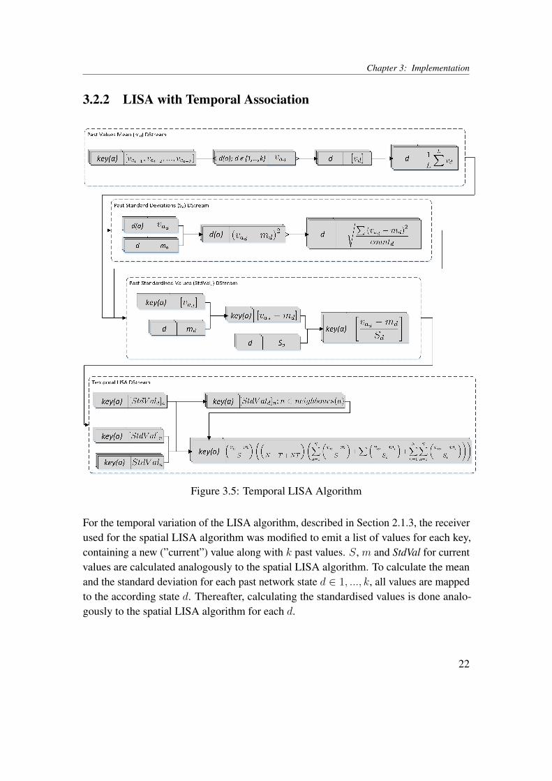
Figure 3.5: Temporal LISA Algorithm

For the temporal variation of the LISA algorithm, described in Section 2.1.3, the receiverused for the spatial LISA algorithm was modified to emit a list of values for each key,containing a new (”current”) value along with k past values. S, m and StdVal for currentvalues are calculated analogously to the spatial LISA algorithm. To calculate the meanand the standard deviation for each past network state d ∈ 1, ..., k, all values are mappedto the according state d. Thereafter, calculating the standardised values is done analo-gously to the spatial LISA algorithm for each d.

22

Chapter 3: Implementation

As the current as well as the past neighbour values are necessary for calculating thetemporal LISA values (cf. Figure 2.2), the mapping of the neighbours’ keys describedin the previous sections is also applied to every d. Finally, all resulting DStreams arecombined to calculate the results.

3.2.3 Spatial Monte Carlo Simulation

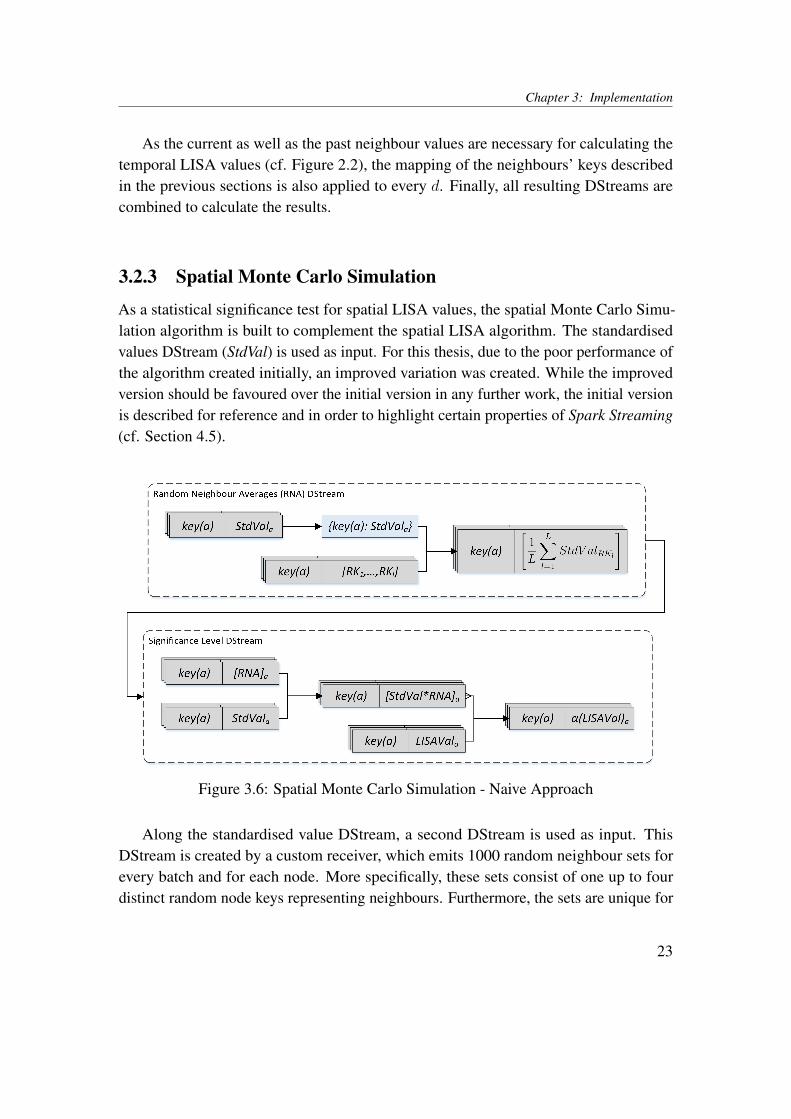
As a statistical significance test for spatial LISA values, the spatial Monte Carlo Simu-lation algorithm is built to complement the spatial LISA algorithm. The standardisedvalues DStream (StdVal) is used as input. For this thesis, due to the poor performance ofthe algorithm created initially, an improved variation was created. While the improvedversion should be favoured over the initial version in any further work, the initial versionis described for reference and in order to highlight certain properties of Spark Streaming(cf. Section 4.5).

Figure 3.6: Spatial Monte Carlo Simulation - Naive Approach

Along the standardised value DStream, a second DStream is used as input. ThisDStream is created by a custom receiver, which emits 1000 random neighbour sets forevery batch and for each node. More specifically, these sets consist of one up to fourdistinct random node keys representing neighbours. Furthermore, the sets are unique for

23

Chapter 3: Implementation

every batch and node i.e. they are distinct combinations of node keys.The two variations of the algorithm mentioned above differ in the way one of the in-termediate results is calculated, namely the averages of the random neighbour values.In both versions, firstly all standardised values of a batch are materialised at one node(blue box in figures 3.6 and 3.7). In the initial version of the algorithm, the resulting mapis thereafter mapped to each of the random neighbour key sets, allowing the averagesof the random neighbour values to be calculated directly. In the improved approach,however, the resulting map is mapped to each of the node keys. The resulting DStreamthus contains the complete key-value map in this batch at each node key, which allowsall subsequent calculation to run in parallel without dependencies between DStreampartitions. To calculate the average neighbour values, this DStream is thereafter joinedwith the DStream containing the random neighbour key sets.

Figure 3.7: Spatial Monte Carlo Simulation - Improved Approach

Finally, in both versions of the algorithm the Random Neighbour Averages (RNA)DStream is joined with the initial input DStream and with the LISAVal DStream resultingfrom the spatial LISA algorithm in order to calculate the random LISA values. To obtainthe significance level for these LISA values, the hypothetical position of the values in theaccording sequence of random LISA values is used. For example, if a LISA value wouldbe entered in the sequence at position 996, the significance level α for this LISA valuewould be α = 996

1001≈ 0.995, or 99.5%.

24

Chapter 3: Implementation

3.2.4 Temporal Monte Carlo Simulation

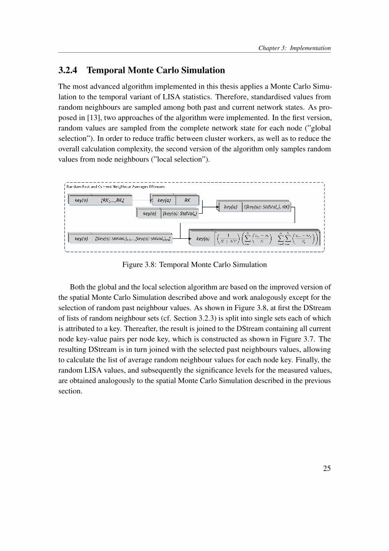
The most advanced algorithm implemented in this thesis applies a Monte Carlo Simu-lation to the temporal variant of LISA statistics. Therefore, standardised values fromrandom neighbours are sampled among both past and current network states. As pro-posed in [13], two approaches of the algorithm were implemented. In the first version,random values are sampled from the complete network state for each node (”globalselection”). In order to reduce traffic between cluster workers, as well as to reduce theoverall calculation complexity, the second version of the algorithm only samples randomvalues from node neighbours (”local selection”).

Figure 3.8: Temporal Monte Carlo Simulation

Both the global and the local selection algorithm are based on the improved version ofthe spatial Monte Carlo Simulation described above and work analogously except for theselection of random past neighbour values. As shown in Figure 3.8, at first the DStreamof lists of random neighbour sets (cf. Section 3.2.3) is split into single sets each of whichis attributed to a key. Thereafter, the result is joined to the DStream containing all currentnode key-value pairs per node key, which is constructed as shown in Figure 3.7. Theresulting DStream is in turn joined with the selected past neighbours values, allowingto calculate the list of average random neighbour values for each node key. Finally, therandom LISA values, and subsequently the significance levels for the measured values,are obtained analogously to the spatial Monte Carlo Simulation described in the previoussection.

25

Chapter 3: Implementation

1 val randomNeighbourAvgs = allRandomLisaValues.map(t => {2 val pastValuesSize = t._2._2.values.head.size3 val filteredMap = t._2._2.filter(me => me._1 != t._1)4

5

6 val randomPastValues: List[Double] = (for (i <- 0 until pastValuesSize) yield7 (for (_ <- 1 to new Random().nextInt(4)+1) yield8 new Random().shuffle(filteredMap.values).head(i)).toList).toList.flatten9

10 val randomCurrentValues: List[Double] = t._2._1._111 .filter(me => t._2._1._2.contains(me._1)).values.toList12 val allRandomValues: List[Double] = randomCurrentValues ++ randomPastValues13 (t._1, allRandomValues.foldLeft(0.0)(_+_)/14 allRandomValues.foldLeft(0.0)((r,c) => r+1))15 })

Listing 2: Global Selection of Random Past Neighbour Values

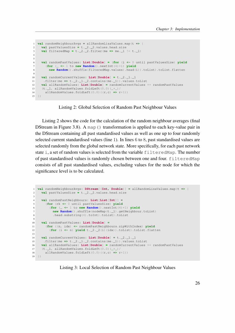
Listing 2 shows the code for the calculation of the random neighbour averages (finalDStream in Figure 3.8). A map() transformation is applied to each key-value pair inthe DStream containing all past standardised values as well as one up to four randomlyselected current standardised values (line 1). In lines 6 to 8, past standardised values areselected randomly from the global network state. More specifically, for each past networkstate i, a set of random values is selected from the variable filteredMap. The numberof past standardised values is randomly chosen between one and four. filteredMapconsists of all past standardised values, excluding values for the node for which thesignificance level is to be calculated.

1 val randomNeighbourAvgs: DStream[(Int, Double)] = allRandomLisaValues.map(t => {2 val pastValuesSize = t._2._2.values.head.size3

4 val randomPastNeighbours: List[List[Int]] =5 (for (rk <- 0 until pastValuesSize) yield6 (for (_ <- 1 to new Random().nextInt(4)+1) yield7 new Random().shuffle(nodeMap(t._1).getNeighbour.toList)8 .head.substring(4).toInt).toList).toList9

10 val randomPastValues: List[Double] =11 (for ((n, idx) <- randomPastNeighbours.zipWithIndex) yield12 (for (i <- n) yield t._2._2(i)(idx)).toList).toList.flatten13

14 val randomCurrentValues: List[Double] = t._2._1._115 .filter(me => t._2._1._2.contains(me._1)).values.toList16 val allRandomValues: List[Double] = randomCurrentValues ++ randomPastValues17 (t._1, allRandomValues.foldLeft(0.0)(_+_)/18 allRandomValues.foldLeft(0.0)((r,c) => r+1))19 })

Listing 3: Local Selection of Random Past Neighbour Values

26

Chapter 3: Implementation

In contrast to the global selection algorithm, the local selection algorithm considersactual neighbouring nodes for the selection of past random neighbour values only. Asshown in listing 3, the map() operation used is very similar to the global selectionalgorithm. However, instead of selecting values from the complete network, random setsof node keys are selected among the node’s actual neighbours for each i (lines 4 to 7).Thereafter, values from this list are obtained according to these keys (lines 9 and 10, cf.Section 2.1.4).

27

4Experiments

This chapter explains the setting, the parameters and the results of the experimentsconducted for each of the algorithms described in the preceding chapter. In particular,the test bed and input data is explained, along with performance measurements and theaccording interpretations for each of the scenarios examined.

4.1 Setting

4.1.1 Test Bed

As a test bed for evaluating the performance of Spark Streaming on LISA statics calcu-lation, a Hadoop YARN cluster of 16 nodes managed by Cloudera Manager v5.1 wasused. The specifications of the cluster nodes are shown in Table 4.1. For submittingapplications to Spark Streaming, the spark-submit command with the parameter--master yarn-cluster was used, which initiates the Spark driver to run as anapplication master managed by YARN [1].

28

Chapter 4: Experiments

Component Node Type 1 Node Type 2

CPU i7-2600 - 2 core i7-4770 - 4 coreRAM 32 GB 32 GBHarddisks 1 x 500 GB 2 x 500 GBQuantity 12 4

Table 4.1: Cluster Node Specifications (adapted from [20])

4.1.2 Topology

For comparability, all experiments were conducted with the same topology (hereaftercalled ”standard topology”) where not mentioned otherwise. It consists of 1600 nodes,and forms a connected graph. As explained in Section 2.1, all connections in the graphsare assigned a weight of 1, and are hence treated as equal in the calculations.

4.1.3 Input / Output

The input data used for all experiments was continuously generated by a custom Sparkreceiver at a certain rate. Where not mentioned otherwise, the rate corresponds to theselected batch duration insofar as for every node, a single value per batch is generated.The values are generated randomly using a Gaussian distribution with a mean of 0.0 anda standard deviation of 1.0 (cf. section 3.1.2) [2].During each experiment execution, all generated input values, as well as the accordingcalculated output values, were stored on a HDFS location. Furthermore, for the evaluationof calculation durations, the log file of the Spark driver node was taken into consideration.

4.2 Spatial LISA Calculation

The first experiment conducted was the calculation of the local Moran’s I, or spatialLISA, as described in Section 3.2.1. At a first stage, the LISA algorithm was run withthe standard topology, at a rate of 20 values per second and an according window lengthof 3 seconds. The goal of this experiment was to show how the number of cluster nodesused influence the time needed for each batch to be calculated. Separate runs for one,two, four, eight and 16 cluster nodes were evaluated.

29

Chapter 4: Experiments

Figure 4.1: Single LISA Run for 1 and 16 Nodes

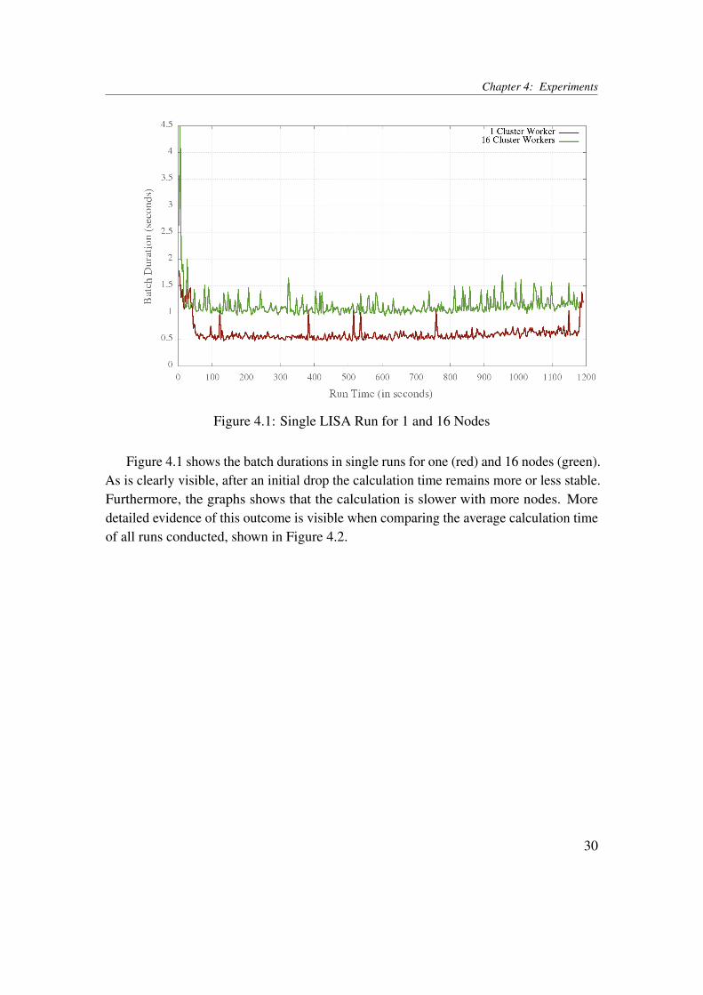
Figure 4.1 shows the batch durations in single runs for one (red) and 16 nodes (green).As is clearly visible, after an initial drop the calculation time remains more or less stable.Furthermore, the graphs shows that the calculation is slower with more nodes. Moredetailed evidence of this outcome is visible when comparing the average calculation timeof all runs conducted, shown in Figure 4.2.

30

Chapter 4: Experiments

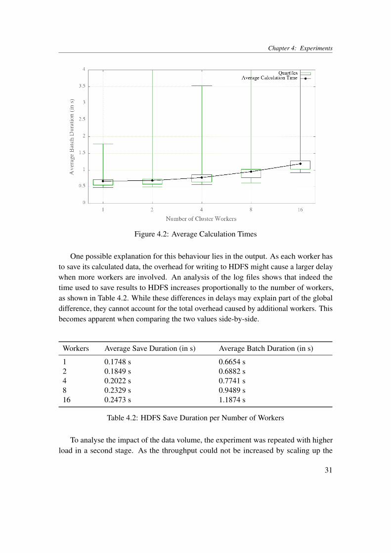
Figure 4.2: Average Calculation Times

One possible explanation for this behaviour lies in the output. As each worker hasto save its calculated data, the overhead for writing to HDFS might cause a larger delaywhen more workers are involved. An analysis of the log files shows that indeed thetime used to save results to HDFS increases proportionally to the number of workers,as shown in Table 4.2. While these differences in delays may explain part of the globaldifference, they cannot account for the total overhead caused by additional workers. Thisbecomes apparent when comparing the two values side-by-side.

Workers Average Save Duration (in s) Average Batch Duration (in s)

1 0.1748 s 0.6654 s2 0.1849 s 0.6882 s4 0.2022 s 0.7741 s8 0.2329 s 0.9489 s16 0.2473 s 1.1874 s

Table 4.2: HDFS Save Duration per Number of Workers

To analyse the impact of the data volume, the experiment was repeated with higherload in a second stage. As the throughput could not be increased by scaling up the

31

Chapter 4: Experiments

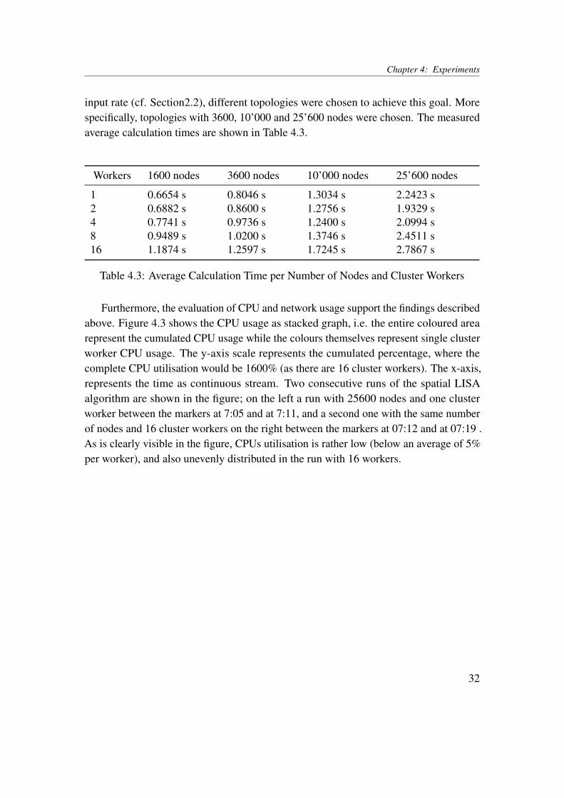
input rate (cf. Section2.2), different topologies were chosen to achieve this goal. Morespecifically, topologies with 3600, 10’000 and 25’600 nodes were chosen. The measuredaverage calculation times are shown in Table 4.3.

Workers 1600 nodes 3600 nodes 10’000 nodes 25’600 nodes

1 0.6654 s 0.8046 s 1.3034 s 2.2423 s2 0.6882 s 0.8600 s 1.2756 s 1.9329 s4 0.7741 s 0.9736 s 1.2400 s 2.0994 s8 0.9489 s 1.0200 s 1.3746 s 2.4511 s16 1.1874 s 1.2597 s 1.7245 s 2.7867 s

Table 4.3: Average Calculation Time per Number of Nodes and Cluster Workers

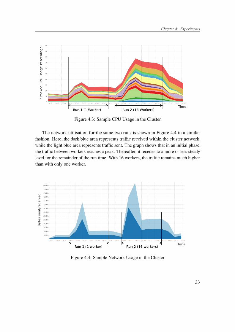
Furthermore, the evaluation of CPU and network usage support the findings describedabove. Figure 4.3 shows the CPU usage as stacked graph, i.e. the entire coloured arearepresent the cumulated CPU usage while the colours themselves represent single clusterworker CPU usage. The y-axis scale represents the cumulated percentage, where thecomplete CPU utilisation would be 1600% (as there are 16 cluster workers). The x-axis,represents the time as continuous stream. Two consecutive runs of the spatial LISAalgorithm are shown in the figure; on the left a run with 25600 nodes and one clusterworker between the markers at 7:05 and at 7:11, and a second one with the same numberof nodes and 16 cluster workers on the right between the markers at 07:12 and at 07:19 .As is clearly visible in the figure, CPUs utilisation is rather low (below an average of 5%per worker), and also unevenly distributed in the run with 16 workers.

32

Chapter 4: Experiments

Figure 4.3: Sample CPU Usage in the Cluster

The network utilisation for the same two runs is shown in Figure 4.4 in a similarfashion. Here, the dark blue area represents traffic received within the cluster network,while the light blue area represents traffic sent. The graph shows that in an initial phase,the traffic between workers reaches a peak. Thereafter, it recedes to a more or less steadylevel for the remainder of the run time. With 16 workers, the traffic remains much higherthan with only one worker.

Figure 4.4: Sample Network Usage in the Cluster

33

Chapter 4: Experiments

In order to interpret these results, the structure of the local Moran’s I and of theaccording algorithm (sections 2.1 and 3.2.1) have to be considered in detail. As depictedin Figure 3.4, both the mean and the standard deviation depend on the complete set ofmeasurements taken during a batch interval. While the reduce() transformations usedin the algorithm are partially parallelisable, all intermediate results have to be collectedat the driver node, and redistributed to the workers for subsequent steps of the algorithmin order to produce to final results (e.g. the mean of all values). The increased networktraffic in the run with 16 workers reflects this result.In addition, the low CPU utilisation described above leads to a possible explanation ofthe performance behaviour. As the calculations in the algorithm are very simple, theoverhead of parallelisation may outweigh the achieved gain in calculation performancefrom the additional cluster workers. Consequently, the behaviour is consistent indepen-dently of the load with which the algorithm is run.

4.3 LISA with Temporal Association

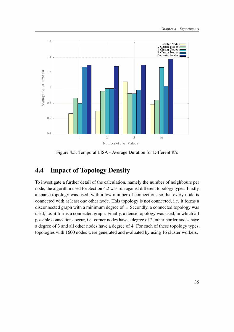
Similar to the first stage of the experiment described above, the algorithm for calculatingLISA with temporal association was run on Spark for the standard topology, with arate of 20 values per minute and and a window duration of 3 seconds. In addition, thenumbers of past sensor values to be included (k) were chosen as 1, 2, 5 and 10. Figure 4.5depicts the average calculation times measured for these k different values, includingk=0 (LISA without temporal association) as reference. Similar to the results described inthe previous section, the calculation time does increase with a larger number of workers.In addition, the number of additional values in the calculation (k) does not influence theperformance in any significant way.

34

Chapter 4: Experiments

Figure 4.5: Temporal LISA - Average Duration for Different K’s

4.4 Impact of Topology Density

To investigate a further detail of the calculation, namely the number of neighbours pernode, the algorithm used for Section 4.2 was run against different topology types. Firstly,a sparse topology was used, with a low number of connections so that every node isconnected with at least one other node. This topology is not connected, i.e. it forms adisconnected graph with a minimum degree of 1. Secondly, a connected topology wasused, i.e. it forms a connected graph. Finally, a dense topology was used, in which allpossible connections occur, i.e. corner nodes have a degree of 2, other border nodes havea degree of 3 and all other nodes have a degree of 4. For each of these topology types,topologies with 1600 nodes were generated and evaluated by using 16 cluster workers.

35

Chapter 4: Experiments

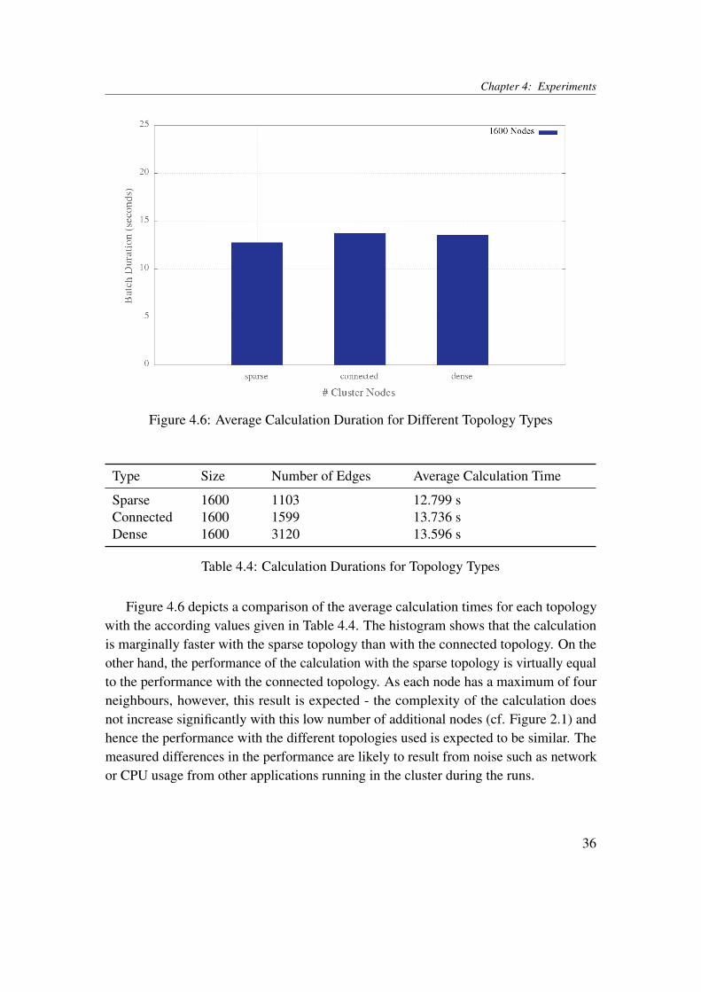
Figure 4.6: Average Calculation Duration for Different Topology Types

Type Size Number of Edges Average Calculation Time

Sparse 1600 1103 12.799 sConnected 1600 1599 13.736 sDense 1600 3120 13.596 s

Table 4.4: Calculation Durations for Topology Types

Figure 4.6 depicts a comparison of the average calculation times for each topologywith the according values given in Table 4.4. The histogram shows that the calculationis marginally faster with the sparse topology than with the connected topology. On theother hand, the performance of the calculation with the sparse topology is virtually equalto the performance with the connected topology. As each node has a maximum of fourneighbours, however, this result is expected - the complexity of the calculation doesnot increase significantly with this low number of additional nodes (cf. Figure 2.1) andhence the performance with the different topologies used is expected to be similar. Themeasured differences in the performance are likely to result from noise such as networkor CPU usage from other applications running in the cluster during the runs.

36

Chapter 4: Experiments

4.5 LISA with Monte Carlo Simulation

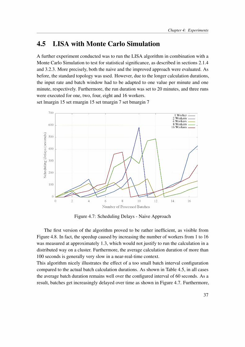
A further experiment conducted was to run the LISA algorithm in combination with aMonte Carlo Simulation to test for statistical significance, as described in sections 2.1.4and 3.2.3. More precisely, both the naive and the improved approach were evaluated. Asbefore, the standard topology was used. However, due to the longer calculation durations,the input rate and batch window had to be adapted to one value per minute and oneminute, respectively. Furthermore, the run duration was set to 20 minutes, and three runswere executed for one, two, four, eight and 16 workers.set lmargin 15 set rmargin 15 set tmargin 7 set bmargin 7

Figure 4.7: Scheduling Delays - Naive Approach

The first version of the algorithm proved to be rather inefficient, as visible fromFigure 4.8. In fact, the speedup caused by increasing the number of workers from 1 to 16was measured at approximately 1.3, which would not justify to run the calculation in adistributed way on a cluster. Furthermore, the average calculation duration of more than100 seconds is generally very slow in a near-real-time context.This algorithm nicely illustrates the effect of a too small batch interval configurationcompared to the actual batch calculation durations. As shown in Table 4.5, in all casesthe average batch duration remains well over the configured interval of 60 seconds. As aresult, batches get increasingly delayed over time as shown in Figure 4.7. Furthermore,

37

Chapter 4: Experiments

at some point values which arrived during different intervals were processed in a singleinterval, which lead to incorrect results for the calculations. To address this issue, thebatch duration would have had to be adjusted to over 100 seconds, which is not desirablefor near-real time analytics of WDN sensor data. Hence, the algorithm was evaluated indetail in order to find improvements.The job details, provided by Spark UI, indicated that one operation could be the un-derlying cause for the poor performance of the algorithm. This was confirmed by ananalysis of the according log files. The mapValues() operation used to create valuessatisfying 1

N

∑Nn=1 StdV alrkn for each key took on average 131.3 seconds for 1 worker,

and 99.0 seconds for 16 workers. This accounts for the largest part of the calculation time.The according average calculation durations are depicted in Figure 4.8, representing thevalues listed in Table 4.5. Due to these results, the algorithm was adapted as discussed inSection 3.2.3.

Figure 4.8: Monte Carlo Simulation Performance - Naive Approach

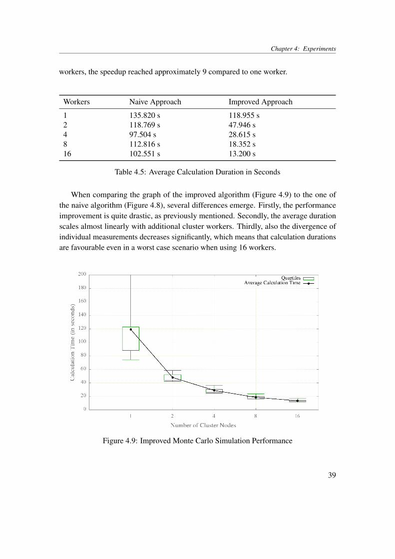
In contrast to the simple LISA calculations as well as to the naive approach presentedabove, the measured calculation durations in case of the improved Monte Carlo Simu-lation algorithm were more aligned with the expectation of a performance gain for anincreasing number of workers (as depicted in Figure 4.9). As the averages in Table 4.5show, a speedup of approximately 2.5 resulted from adding a second worker. With 16

38

Chapter 4: Experiments

workers, the speedup reached approximately 9 compared to one worker.

Workers Naive Approach Improved Approach

1 135.820 s 118.955 s2 118.769 s 47.946 s4 97.504 s 28.615 s8 112.816 s 18.352 s16 102.551 s 13.200 s

Table 4.5: Average Calculation Duration in Seconds

When comparing the graph of the improved algorithm (Figure 4.9) to the one ofthe naive algorithm (Figure 4.8), several differences emerge. Firstly, the performanceimprovement is quite drastic, as previously mentioned. Secondly, the average durationscales almost linearly with additional cluster workers. Thirdly, also the divergence ofindividual measurements decreases significantly, which means that calculation durationsare favourable even in a worst case scenario when using 16 workers.

Figure 4.9: Improved Monte Carlo Simulation Performance

39

Chapter 4: Experiments

4.6 LISA with Temporal Association and Monte CarloSimulation

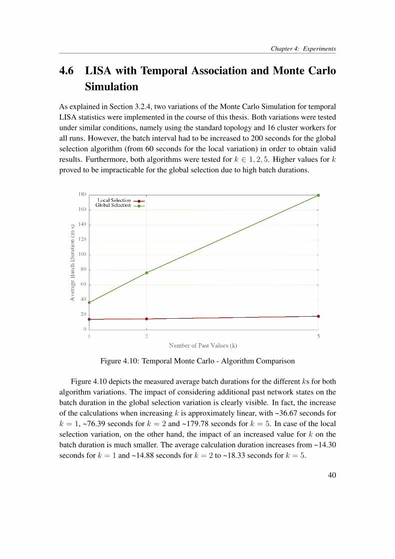
As explained in Section 3.2.4, two variations of the Monte Carlo Simulation for temporalLISA statistics were implemented in the course of this thesis. Both variations were testedunder similar conditions, namely using the standard topology and 16 cluster workers forall runs. However, the batch interval had to be increased to 200 seconds for the globalselection algorithm (from 60 seconds for the local variation) in order to obtain validresults. Furthermore, both algorithms were tested for k ∈ 1, 2, 5. Higher values for kproved to be impracticable for the global selection due to high batch durations.

Figure 4.10: Temporal Monte Carlo - Algorithm Comparison

Figure 4.10 depicts the measured average batch durations for the different ks for bothalgorithm variations. The impact of considering additional past network states on thebatch duration in the global selection variation is clearly visible. In fact, the increaseof the calculations when increasing k is approximately linear, with ~36.67 seconds fork = 1, ~76.39 seconds for k = 2 and ~179.78 seconds for k = 5. In case of the localselection variation, on the other hand, the impact of an increased value for k on thebatch duration is much smaller. The average calculation duration increases from ~14.30seconds for k = 1 and ~14.88 seconds for k = 2 to ~18.33 seconds for k = 5.

40

Chapter 4: Experiments

While the results for the global selection algorithm may seem to indicate bad overallperformance, they are explicable and to be expected: for each additional network state,a full Monte Carlo Simulation has to be performed in which the complete global statehas to be considered for each node value (cf. Section 4.5). This leads to a high levelof wide dependencies in the computation graph of the algorithm, which in turn leads tolong calculation durations.

41

5Conclusion

In chapters 3 and 4, both the implementation of LISA statistics on Spark Streamingand the performance of this implementation were discussed. It was shown that theimplementation of algorithms for calculating LISA indicators and according statisticaltests are feasible with Spark Streaming. Furthermore, the performance evaluation showedthat the majority of these calculations can be run with reasonable performance in a nearreal-time manner.The main conclusions which can be drawn from the implementation of this thesis istwofold. On the one hand, the high level API provided by Spark Streaming allowed forsimple algorithms for LISA calculations. Even in the most complex case, namely thetemporal Monte Carlo Simulation, the algorithm could be implemented on a moderatecomplexity level. On the other hand, recreating the WDN metering scenario describedin [13] proved to be difficult mainly due to the characteristics of Spark Streamings datainput API. This lead to several abstractions in the application architecture.The performance evaluation for the LISA calculations have showed that Spark Streamingis well suited to handle the workload generated by a WDN even on a small cluster. Thespatial LISA algorithm was run in various scenarios, namely with different numbers ofnodes and different topology types in terms of the amount of connections. Furthermore,the performance impact of considering past network states was measured by runningseveral configurations of the temporal LISA algorithm. In all cases, the calculation

42

Chapter 5: Conclusion

duration per batch remained in a range which would easily allow for an ad-hoc analysisin a real-world WDN scenario.However, one peculiarity was found when comparing different numbers of cluster work-ers. The results showed decreasing performance with additional cluster workers. Thiseffect may result from the nature of LISA indicators as the calculation of both the stan-dard deviation and the mean requires knowledge of the complete network state, whichleads to unfavourable wide dependencies. Further work will be required to fully clarifythis issue, as discussed in the subsequent section.The evaluation of the statistical tests yielded more divergent results. In the spatial varia-tion, reasonable delays were achieved with an algorithm adapted to the characteristics ofSpark. The temporal variation of the algorithm, on the other hand, proved to performpoorly due to its dependency on the complete current and past network states. Reasonableperformance could only be achieved with an adjustment proposed by [13].

5.1 Future Work

The problem covered by this thesis is very specific in terms of both technology (SparkStreaming) and of applicability to a real-world scenario (WDN). However, its scope hadto be confined considerably. Consequently, there are many possibilities for improvementsand further work. These include improvements of the algorithms and of the architecture,as well as the adaptation towards a realistic scenario.As shown in Chapter 3, statistical algorithms are a central part of the implementation.As they were mainly developed as a proof of concept of using Spark Streaming forsuch calculations, they are in no way optimised for performance. Improvements couldinclude a better adaptation to the characteristics of Spark Streaming, and to data-parallelcalculations in general, as well as the exploitation of data locality.In addition, while the implementation architecture is based on the scenario describedby [13], many adjustments and abstractions had to be made. Clearly, an interestingcomplement to this thesis would be to integrate the implementation into this scenariowith less adjustments and to test it in a real-world setting.A crucial part of such an extension would be an adjustment of the data input architec-ture. Currently, sensor values are simulated with respect to the Spark Streaming batchinterval as discussed in Section 3.1.2. Sensors deployed in WDNs, however, do not emitmeasurements in a synchronised fashion. In consequence, calculation results could befalsified if multiple values measured by a single sensor would be processed within one

43

Chapter 5: Conclusion

batch. A possible solution to this issue could be the use of input values which are anaverage of sensor measurements over a certain time span as input values.In conclusion, this thesis has shown that Spark Streaming is suitable for anomaly de-tection in the context of sensors deployed in a WDN, but there is still much room forimprovement and extension.

44

Bibliography

[1] Running spark on yarn. ”http://spark.apache.org/docs/1.0.0/running-on-yarn.html#configuration”. ”[Online; accessed 10-30-2014]”.

[2] Spark api. ”http://www.scala-lang.org/api/current/index.html#scala.util.Random”. ”[Online; accessed 09-24-2014]”.

[3] Spark streaming programming guide. ”http://spark.apache.org/docs/latest/streaming-programming-guide.html”. ”[Online; accessed10-05-2014]”.

[4] The apache software foundation announces apache spark as a top-levelproject. ”https://blogs.apache.org/foundation/entry/the_apache_software_foundation_announces50”, 2014. ”[Online; ac-cessed 09-23-2014]”.

[5] Apache spark vs. apache storm. ”http://stackoverflow.com/a/24125900”, 2014. ”[Online; accessed 10-26-2014]”.

[6] Data parallelism. ”http://en.wikipedia.org/wiki/Data_parallelism”, 2014. ”[Online; accessed 10-26-2014]”.

[7] Samza - spark streaming. ”http://samza.incubator.apache.org/learn/documentation/0.7.0/comparisons/spark-streaming.

html”, 2014. ”[Online; accessed 11-06-2014]”.

[8] Storm documentation - concepts. ”https://storm.incubator.apache.org/documentation/Concepts.html”, 2014. ”[Online; accessed 10-26-2014]”.

45

Chapter 5: BIBLIOGRAPHY

[9] Storm documentation - rationale. ”https://storm.incubator.apache.org/documentation/Rationale.html”, 2014. ”[Online; accessed 10-25-2014]”.

[10] Storm documentation - tutorial. ”https://storm.incubator.apache.org/documentation/Tutorial.html”, 2014. ”[Online; accessed 10-25-2014]”.

[11] Task parallelism. ”http://en.wikipedia.org/wiki/Task_parallelism”, 2014. ”[Online; accessed 10-26-2014]”.

[12] Luc Anselin. Local indicators of spatial association – LISA. Geographical Analysis,27(2):93–115, 1995.

[13] D.E. Difallah, P. Cudre-Mauroux, and S.A McKenna. Scalable anomaly detectionfor smart city infrastructure networks. Internet Computing, IEEE, 17(6):39–47,Nov 2013.

[14] Pierre Goovaerts and Geoffrey Jacquez. Accounting for regional background andpopulation size in the detection of spatial clusters and outliers using geostatisticalfiltering and spatial neutral models: the case of lung cancer in long island, newyork. International Journal of Health Geographics, 3(1):14, 2004.

[15] Xinh Huynh. Storm vs. spark streaming: Side-by-side compar-ison. ”http://xinhstechblog.blogspot.ch/2014/06/storm-vs-spark-streaming-side-by-side.html”, June 2014.”[Online; accessed 11-06-2014]”.

[16] V. Kalavri and V. Vlassov. Mapreduce: Limitations, optimizations and open issues.In Trust, Security and Privacy in Computing and Communications (TrustCom),2013 12th IEEE International Conference on, pages 1031–1038, July 2013.

[17] Vasiliki Kalavri and Vladimir Vlassov. Mapreduce: Limitations, optimizations andopen issues. In TrustCom/ISPA/IUCC, pages 1031–1038. IEEE, 2013.

[18] Simpal Kumar. Real time data analysis for water distribution network using storm.Master’s thesis, University of Fribourg, May 2014.

[19] Zhiqiang Ma and Lin Gu. The limitation of mapreduce: A probing case and alightweight solution. In CLOUD COMPUTING 2010, The First InternationalConference on Cloud Computing, GRIDs, and Virtualization, pages 68–73, 2010.

46

Chapter 5: BIBLIOGRAPHY

[20] Phokham Nonova. Hdfs blocks placement strategy. Master’s thesis, University ofFribourg, October 2014.

[21] Matei Zaharia, Mosharaf Chowdhury, Tathagata Das, Ankur Dave, Justin Ma,Murphy McCauley, Michael J. Franklin, Scott Shenker, and Ion Stoica. Resilientdistributed datasets: A fault-tolerant abstraction for in-memory cluster computing.In Proceedings of the 9th USENIX Conference on Networked Systems Designand Implementation, NSDI’12, pages 2–2, Berkeley, CA, USA, 2012. USENIXAssociation.

[22] Matei Zaharia, Mosharaf Chowdhury, Michael J. Franklin, Scott Shenker, andIon Stoica. Spark: Cluster computing with working sets. In Proceedings of the2Nd USENIX Conference on Hot Topics in Cloud Computing, HotCloud’10, pages10–10, Berkeley, CA, USA, 2010. USENIX Association.

[23] Matei Zaharia, Tathagata Das, Haoyuan Li, Scott Shenker, and Ion Stoica. Dis-cretized streams: An efficient and fault-tolerant model for stream processing onlarge clusters. In Proceedings of the 4th USENIX Conference on Hot Topicsin Cloud Ccomputing, HotCloud’12, pages 10–10, Berkeley, CA, USA, 2012.USENIX Association.

47

AAppendix

A.1 Complete Source Code

The complete source code resulting from this thesis is available at the following URL:https://github.com/snoooze03/SparkLisa

48

E r k l ä r u n g

gemäss Art. 28 Abs. 2 RSL 05

Name/Vorname: ........................................................................................................

Matrikelnummer: ........................................................................................................

Studiengang: ……………………………………………………………………………

Bachelor Master Dissertation

Titel der Arbeit: ........................................................................................................

........................................................................................................

........................................................................................................

LeiterIn der Arbeit: ........................................................................................................

........................................................................................................

Ich erkläre hiermit, dass ich diese Arbeit selbständig verfasst und keine anderen als die

angegebenen Quellen benutzt habe. Alle Stellen, die wörtlich oder sinngemäss aus Quellen

entnommen wurden, habe ich als solche gekennzeichnet. Mir ist bekannt, dass andernfalls

der Senat gemäss Artikel 36 Absatz 1 Buchstabe r des Gesetztes vom 5. September 1996

über die Universität zum Entzug des auf Grund dieser Arbeit verliehenen Titels berechtigt ist. Ich gewähre hiermit Einsicht in diese Arbeit.

..................................................................

Ort/Datum

.............................................................

Unterschrift