Global Journal of Pure and Applied Mathematics.

ISSN 0973-1768 Volume 13, Number 10 (2017), pp. 7111-7122

© Research India Publications

http://www.ripublication.com

SINC BASED METHOD FOR SOLVING TWO-

DIMENSIONAL FREDHOLM INTEGRAL EQUATIONS

Yousef A. Al-Jarrah1 and Mohammed A. Aljarrah2

1,2Department of Mathematics, Tafila Technical University, Tafila – Jordan.

Abstract

Throughout this paper, we study the Sinc collocation method applied to obtain

a numerical solution of two-dimensional Fredholm integral equation of first

and second kinds. This method has been shown a powerful numerical tool for

finding an accurate numerical solution. The Sinc function properties are

provided and the global convergence analysis is given to guarantee the

efficiently of our method. Moreover, we apply the method for some numerical

examples to ensure the validity of the Sinc technique.

Keywords: Fredholm, two-dimensional, Sinc Approximation.

1. INTRODUCTION

Numerous problems in engineering, physics and mechanics are modeled as a two-

dimensional Fredholm integral equations [1], [2]. In particular, the two-dimensional

integral equations appear in electromagnetic, electrodynamic, heat and mass transfer,

population and image processing [3], [4], [5] and [6]. Where the out-of-focus images

are modeled as two-dimensional linear Fredholm integral equation of the first kind,

and by solving the integral equation the given noising images are constructed. So, the

numerical solution of the two-dimensional integral equation took the attention of

many researches, where many different methods are used to solve the integral

equation. For example, Haar wavelet [7], Coiflet wavelet [8] are a new methods based

on the wavelet basis, in [9], Han and Wang approximated the two-dimensional

Fredholm integral equations by the Galerkin iterative method. In addition, Nystrom

7112 Yousef A. Al-Jarrah and Mohammed A. Aljarrah

method [9], collocation method [10], and Gaussian radial basis function [11] are the

commonly methods used.

In this paper, we consider the two-dimensional linear Fredholm integral equation of

the first and second kind respectively of the form

, , , , ,b b

a ag x y k x y s t f s t dsdt (1.1)

, , , , , ,

b b

a af x y g x y k x y s t f s t dsdt (1.2)

Here, ,f x y is the unknown function, we assume that the functions ,f g are

sufficiently smooth for 2 2

, , ,x y a b a b , and , , ,k x y s t is continuous on

2 2

, , , ,x s y t a b a b .

2. SINC FUNCTION

In this section, we will give a brief introduction of the Sinc function and it’s

properties, in addition to some definitions and theorems that are required for function

approximation, where the Sinc function is defined in details in [12]. The Sinc function

is defined in the real line as follows

sin( )

0sinc

1 0

x xx x

x

,

and the normalized Sinc function has the form

sin( ) 0

Sinc( )

1 0

x xx x

x

(2.1)

This function is defined by Borel and Whittaker. For any 0h the Sinc function (2.1)

is translated with spaced nodes jh and scaled by h as follows;

( , ) , 0, 1, 2,... .x jhS j h x Sinc j

h

(2.2)

Definition 1. Let 1(D )EH denote the family of all analytic functions in the infinite

strip

; Im , / 2ED z u iv z v d d .

SINC BASED METHOD FOR SOLVING TWO-DIMENSIONAL FREDHOLM INTEGRAL EQUATIONS 7113

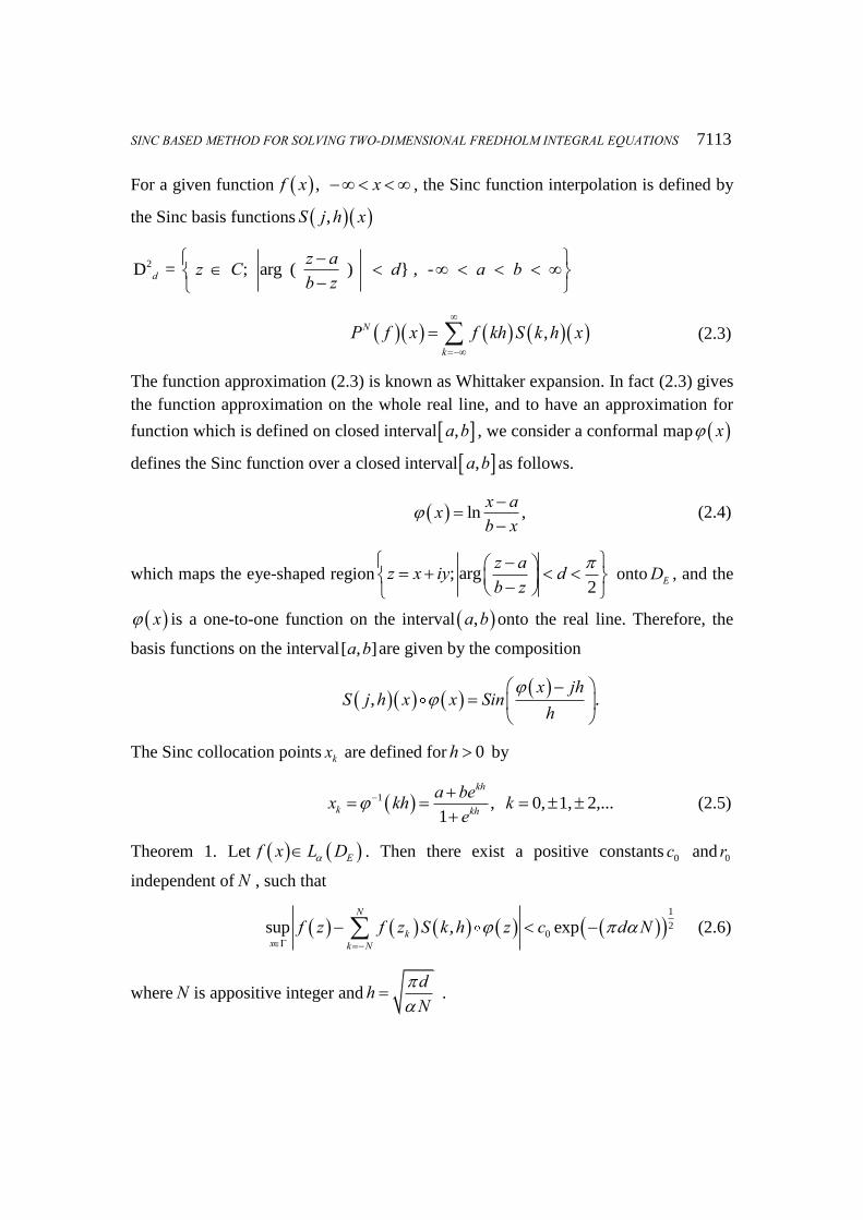
For a given function , f x x , the Sinc function interpolation is defined by

the Sinc basis functions ,S j h x

2D = ; arg ( ) } , - dz az C d a bb z

,N

kP f x f kh S k h x

(2.3)

The function approximation (2.3) is known as Whittaker expansion. In fact (2.3) gives

the function approximation on the whole real line, and to have an approximation for

function which is defined on closed interval ,a b , we consider a conformal map x

defines the Sinc function over a closed interval ,a b as follows.

ln ,x axb x

(2.4)

which maps the eye-shaped region ; arg2

z az x iy db z

onto ED , and the

x is a one-to-one function on the interval ,a b onto the real line. Therefore, the

basis functions on the interval[ , ]a b are given by the composition

, .x jh

S j h x x Sinh

The Sinc collocation points kx are defined for 0h by

1 , 0, 1, 2,...1

kh

k kh

a bex kh ke

(2.5)

Theorem 1. Let Ef x L D . Then there exist a positive constants 0c and 0r

independent of N , such that

1

20sup , exp

N

kx k N

f z f z S k h z c d N

(2.6)

where N is appositive integer anddhN

.

7114 Yousef A. Al-Jarrah and Mohammed A. Aljarrah

For a continuous function ,f x y is on the rectangle 2

,a b , then the Sinc

interpolation is defined as

'

'

, , y , ',N N

N k kk N k N

P f x y f x S k h x S k h y

(2.7)

Where kx and'ky , ' ,...,k k N N are the Sinc collocation points defined in (2.5) and

1

2dhN

. Theorem 2: For a given constants ,d and integer N ,

1

2dhN

, and

NP f x is the Sinc interpolation for the function ,f x y (2.7). Then

2

1 12 2

1 2

, ,

sup , , log expNx y a b

f x y P f x y c c N N d N

(2.8)

Where, 1c and 2c are constants independent of N .

The proof exists in [12]

3. SINC-METHOD FOR TWO-DIMENSIONAL FREDHOLM INTEGRAL

EQUATION

In this section we will use the Sinc basis functions for approximating the unknown

function ,f x y of the integral equations (1.1) and (1.2). Firstly, inserting equation

(2.7) into equation (1.1), we have

, ' '

'

, , , ,N Nb b

k k k ka ak N k N

g x y k x y s t f S s S t dsdt

(3.1)

where , ' , , ' ,...,k kf k k N N are unknowns that need be to determined. Consequently,

substituting the Sinc collocation points ,i ,...,ix N N and , ,...,jy j N N into

equation (3.1) to have the system of linear equations

, ' '

'

, , , ,

, ,...,

N N b b

i j k k i j k ka ak N k N

g x y f k x y s t S s S t dsdt

i j N N

(3.2)

For simplicity, let , ' ', , , ,b b

k k k ka aA x y k x y s t S s S t dsdt , then equation

(3.2) becomes as

SINC BASED METHOD FOR SOLVING TWO-DIMENSIONAL FREDHOLM INTEGRAL EQUATIONS 7115

, ' , '

'

, , , , ,...,N N

i j k k k k i jk N k N

g x y f A x y i j N N

(3.3)

The system (3.3) can be written in the matrix equation

G AF (3.4)

where

1

1 1

, ,g , ,..., , ,

, ,...,g , ,..., ,

N N N N N N

N N N N N N

g x y x y g x yG

g x y x y g x y

(3.5)

1

1 1

, , , ,...,

, , , ,..., , ,..., ,

N N N N

N N N N N N N N

f x y f x yF

f x y f x y f x y f x y

(3.6)

and

, , 1, 1, ,

, 1 , 1 !, 1 !, , 1

, ,

, , , , ... ,

, ... , , , ... ,

. . . . .

.. . . .

.

. .

, ,...

N N N N N N N N N N N N N N N N N N N N

N N N N N N N N N N N N N N N N N N N N

N N N N N N N N

A x y A x y A x y A x y A x yA x y A x y A x y A x y A x y

A

A x y A x y

!, !, ,

. .

, , ... ,N N N N N N N N N N N NA x y A x y A x y

(3.7)

By solving equation (3.4) using inverse method as 1F A G , then we will obtain the

approximation solution for the unknown function ,f x y . In fact, if the matrix A is

singular, then an approximation inverse could be evaluated by using the Pseudo

inverse matrix.

Now, the same process could be used to solve equation (1.2) where thee unknown

function ,f x y of equation (1.2) is approximated by Sinc function interpolation

(2.7), substituting equation (2.7) into equation (1.2), then substituting the Sinc

collocation points ', , , ' ,...,k kx y k k N N to have a linear system of the unknowns

, ' , , ' ,...,k kf k k N N of the form

'

, '

''

,, , ,

, ,...,

N N k i k j

i j k k b bk N k N

i j k ka a

S x S yg x y f

k x y s t S s S t dsdt

i j N N

(3.8)

let

7116 Yousef A. Al-Jarrah and Mohammed A. Aljarrah

, ' ' ', , , ,b b

k k k k k ka aB x y S x S y k x y s t S s S t dsdt

Then the system (3.8) can be written in matrix equation

BG F (3.9)

where.,i jB B

4. CONVERGE ANALYSIS

In this section, we provide the necessary conditions for the convergent of our method

for solving integral equations (1.1) and (1.2), where we proved that the rate of

convergent is O N , the proof of the next theorem based on [13]

Theorem 1. If ,f x y is the exact solution of (1.1) and , , ,k x y s t continuous on

2 2

, ,a b a b , let

, ' '

'

,N N

N NN k k k k

k N k NP f x y f S x S y

(4.1)

Is the Sinc function interpolation of ,f x y , where , ' , , ' ,...,Nk kf k k N N are the

coefficients that are determined by solving the matrix equation (3.4), then

1 1

22 2

2 3 2

4, log exp 1 3 logN

Nf x y P f c c N N d N N

where 1c and 2c are constants independent of N .

Proof: let

, '

'

,N N

N k k k kk N k N

P f x y f S x S y

(4.2)

Be the Sinc interpolation for the function ,f x y where 1 1

, ' , 'k kf f kh k h

the exact values of the function ,f x y at the Sinc collocation points

1 1

', 'k kx kh y k h . Then

N NN N N Nf P f f P f P f P f (4.3)

Now, by substituting equations (4.1) and (4.2) into the integral equation (1.1) we

have the following equations

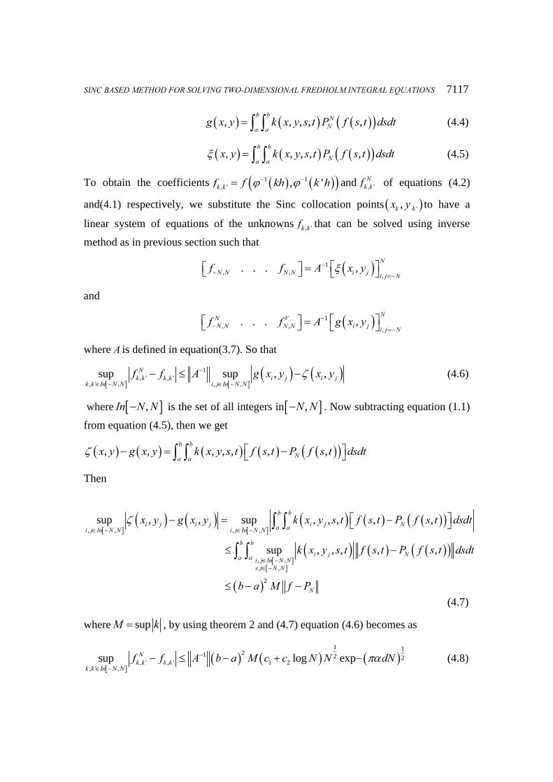
SINC BASED METHOD FOR SOLVING TWO-DIMENSIONAL FREDHOLM INTEGRAL EQUATIONS 7117

, , , , ,b b N

Na ag x y k x y s t P f s t dsdt (4.4)

, , , , ,b b

Na ax y k x y s t P f s t dsdt (4.5)

To obtain the coefficients 1 1

, ' , 'k kf f kh k h and , '

Nk kf of equations (4.2)

and(4.1) respectively, we substitute the Sinc collocation points ',k kx y to have a

linear system of equations of the unknowns, 'k kf that can be solved using inverse

method as in previous section such that

1

, ,,

. . . ,N

N N N N i j i j Nf f A x y

and

1

, ,,

. . . ,NN V

N N N N i j i j Nf f A g x y

where A is defined in equation(3.7). So that

1

, ' , ', ' , , ,

sup sup , ,Nk k k k i j i j

k k In N N i j In N Nf f A g x y x y

(4.6)

where ,In N N is the set of all integers in ,N N . Now subtracting equation (1.1)

from equation (4.5), then we get

, , , , , , ,b b

Na ax y g x y k x y s t f s t P f s t dsdt

Then

, , , ,

, ,

, ,

sup , , sup , , , , ,

sup , , , , ,

b b

i j i j i j Na ai j In N N i j In N N

b b

i j Na a i j In N Ns t N N

x y g x y k x y s t f s t P f s t dsdt

k x y s t f s t P f s t dsdt

2

Nb a M f P

(4.7)

where supM k , by using theorem 2 and (4.7) equation (4.6) becomes as

1 121 2 2

, ' , ' 1 2, ' ,

sup log expNk k k k

k k In N Nf f A b a M c c N N dN

(4.8)

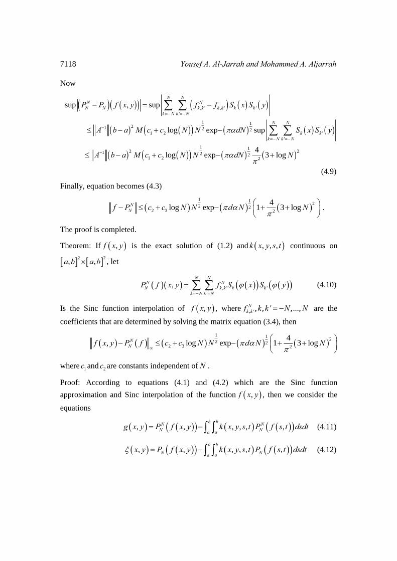
7118 Yousef A. Al-Jarrah and Mohammed A. Aljarrah

Now

, ' , ' '

'

1 121 2 2

1 2 '

'

1 12 21 2 2

1 2 2

sup , sup

log exp sup

4 log exp 3 log

N NN N

N N k k k k k kk N k N

N N

k kk N k N

P P f x y f f S x S y

A b a M c c N N dN S x S y

A b a M c c N N dN N

(4.9)

Finally, equation becomes (4.3)

1 1

22 2

2 3 2

4log exp 1 3 logN

Nf P c c N N d N N

.

The proof is completed.

Theorem: If ,f x y is the exact solution of (1.2) and , , ,k x y s t continuous on

2 2

, ,a b a b , let

, ' '

'

,N N

N NN k k k k

k N k NP f x y f S x S y

(4.10)

Is the Sinc function interpolation of ,f x y , where , ' , , ' ,...,Nk kf k k N N are the

coefficients that are determined by solving the matrix equation (3.4), then

1 1

22 2

2 3 2

4, log exp 1 3 logN

Nf x y P f c c N N d N N

where 1c and 2c are constants independent of N .

Proof: According to equations (4.1) and (4.2) which are the Sinc function

approximation and Sinc interpolation of the function ,f x y , then we consider the

equations

, , , , , ,b bN N

N Na ag x y P f x y k x y s t P f s t dsdt (4.11)

, , , , , ,b b

N Na ax y P f x y k x y s t P f s t dsdt (4.12)

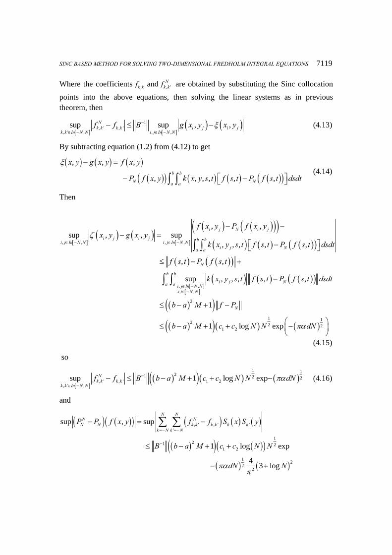
SINC BASED METHOD FOR SOLVING TWO-DIMENSIONAL FREDHOLM INTEGRAL EQUATIONS 7119

Where the coefficients, 'k kf and , '

Nk kf are obtained by substituting the Sinc collocation

points into the above equations, then solving the linear systems as in previous

theorem, then

1

, ' , ', ' , , ,

sup sup , ,Nk k k k i j i j

k k In N N i j In N Nf f B g x y x y

(4.13)

By subtracting equation (1.2) from (4.12) to get

, , ,

, , , , , ,b b

N Na a

x y g x y f x y

P f x y k x y s t f s t P f s t dsdt

(4.14)

Then

, , , ,

, ,sup , , sup

, , , , ,

, ,

i j N i j

i j i j b bi j In N N i j In N Ni j Na a

N

f x y P f x yx y g x y

k x y s t f s t P f s t dsdt

f s t P f s t

, ,

, ,

2

1 12

2 21 2

sup , , , , ,

1

1 log exp

b b

i j Na a i j In N Ns t N N

N

k x y s t f s t P f s t dsdt

b a M f P

b a M c c N N dN

(4.15)

so

1 121 2 2

, ' , ' 1 2, ' ,

sup 1 log expNk k k k

k k In N Nf f B b a M c c N N dN

(4.16)

and

, ' , ' '

'

121 2

1 2

12

22

sup , sup

1 log exp

43 log

N NN N

N N k k k k k kk N k N

P P f x y f f S x S y

B b a M c c N N

dN N

7120 Yousef A. Al-Jarrah and Mohammed A. Aljarrah

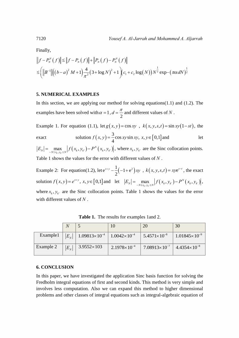
Finally,

1 1

2 21 2 21 22

41 3 log 1 log exp

N NN N N Nf P f f P f P f P f

B b a M N c c N N dN

5. NUMERICAL EXAMPLES

In this section, we are applying our method for solving equations(1.1) and (1.2). The

examples have been solved with 1 ,2

d and different values of N .

Example 1. For equation (1.1), let , cosg x y xy , , , , sin 1k x y s t xy st , the

exact solution 3

, cos sin , , 0,14

f x y xy xy x y and let

'

' ',

max , ,k k

NN k k k kN x y N

E f x y P x y

, where ',k kx y are the Sinc collocation points.

Table 1 shows the values for the error with different values of N .

Example 2: For equation(1.2), let 21e 1 e

2

x y xy , , , , es tk x y s t xy , the exact

solution , , , 0,1x yf x y e x y and let '

' ',

max , ,k k

NN k k k kN x y N

E f x y P x y

,

where ',k kx y are the Sinc collocation points. Table 1 shows the values for the error

with different values of N .

Table 1. The results for examples 1and 2.

N 5 10 20 30

Example1 NE

41.09813 10 41.0042 10 85.4571 10 91.01845 10

Example 2 NE 3.9552 103 42.1978 10 77.08913 10 84.4354 10

6. CONCLUSION

In this paper, we have investigated the application Sinc basis function for solving the

Fredholm integral equations of first and second kinds. This method is very simple and

involves less computation. Also we can expand this method to higher dimensional

problems and other classes of integral equations such as integral-algebraic equation of

SINC BASED METHOD FOR SOLVING TWO-DIMENSIONAL FREDHOLM INTEGRAL EQUATIONS 7121

index-1 and index-2. Note that, for applying this method we need to solve the linear

system of equations, and the Pseudo inverse could be use if the coefficient matrix is

singular.

REFERENCES

[1] K. Atkinson, The Numeerical Solution of Integral Equations of Second Kind,

Cambridge University, 1997.

[2] A.J.Jerri, Introduction to Integral Equations with Applications, John Wilwy and

Sons: INC, 1999.

[3] S. S. M.V.K. Chari, Numerical Methods in Electromagnetism, Academic Press,

2000.

[4] Z. Cheng, "Quantum effects of thermal radiation in a Kerr nonlinear blackbody,"

Journal of the Optical Society of America, vol. B, no. 19, pp. 1692-1705, 2002.

[5] T. I. Y. Liu, "Integral equation theories for predicting water structure,"

Biophysical Chemistry, vol. 78, pp. 97-111, 1999.

[6] D. W. Q. Tang, "An integral equation describing an asexual population,"

Nonlinear Analysis,, vol. 53, pp. 683-699, 2003.

[7] Abdollah Borhanifar, Khadijeh Sadri, "Numerical Solution for Systems of Two

Dimensional Integral Equations by Using Jacobi Operational Collocation

Method," Sohag J. Math, vol. 1, no. 1, pp. 15-26, 2014.

[8] E.-B. L. Yousef A-ljarrah, "Wavelet Based Method for Solving Two-

Dimensional Integral Equations," Mathematica Antena, 2015.

[9] H. Guoqiang, W. Jiong, "Extrapolation of Nystrom Solution for Two-

Dimensional Nonlinear Fredholm Integral Equation," Journal of Computaional and Applied Mathematics, vol. 134, pp. 259-268, 2001.

[10] F. L. W.J. Wie, "A Fast Numerical Solution Method for two Dimensional

Fredholm Integral Equations of the Second Kind," Applied Mathematical Compuation, vol. 59, pp. 1709-1719, 2009.

[11] S. E. Amjad Alipanah, "Numerical Solution of the Two-Dimensional Fredholm

Interal Equations Using Gaussian Basis Function," Journal of Computational and Applied Mathematics, vol. 235, pp. 5342-5347, 2011.

7122 Yousef A. Al-Jarrah and Mohammed A. Aljarrah

[12] F. Stenger, Numerical Methods Based on Sinc and Analytic Functions, New

York: Springer, 1993.

[13] R. M. T. a. M. A. Khosrow Maleknejad, "Solution of First kind Fredholm

Integral Equation by Sinc Function," International Journal of Mathematical, Computational, Physical, Electrical and Computer Engineering, vol. 4, no. 6, pp.

737-741, 2010.