Sylwia Trzaska

•IRI: Steve Zebiak, Lisa Goddard, Simon Mason, Tony Barnston, Madeleine Thomson, Neil Ward, Ousmane N’Diaye and many others•ECMWF: Magdalena Balmaseda•Meteo-France: J.-P. Céron

Climate Risk Management: Climate Risk Management: Seasonal Climate PredictionSeasonal Climate Prediction

•IRI: Linking Climate and Society•Climate Prediction•Seasonal Climate Forecast•Use of Ocean Data•Importance of ARGO data

Climate Information & Climate Prediction Tool

Climate Risk Management: Climate Risk Management: Seasonal Climate PredictionSeasonal Climate Prediction

Linking Science to SocietyLinking Science to Society

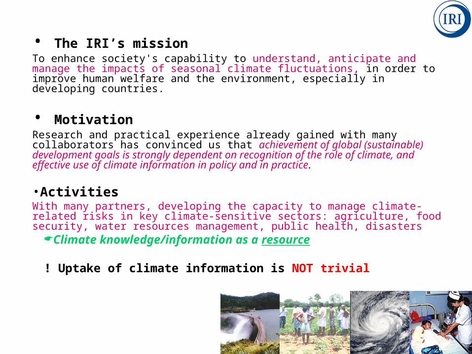
• The IRI’s missionTo enhance society's capability to understand, anticipate and manage the impacts of seasonal climate fluctuations, in order to improve human welfare and the environment, especially in developing countries.

• MotivationResearch and practical experience already gained with many collaborators has convinced us that achievement of global (sustainable) development goals is strongly dependent on recognition of the role of climate, and effective use of climate information in policy and in practice.

•ActivitiesWith many partners, developing the capacity to manage climate-related risks in key climate-sensitive sectors: agriculture, food security, water resources management, public health, disasters

Climate knowledge/information as a resource

! Uptake of climate information is NOT trivial

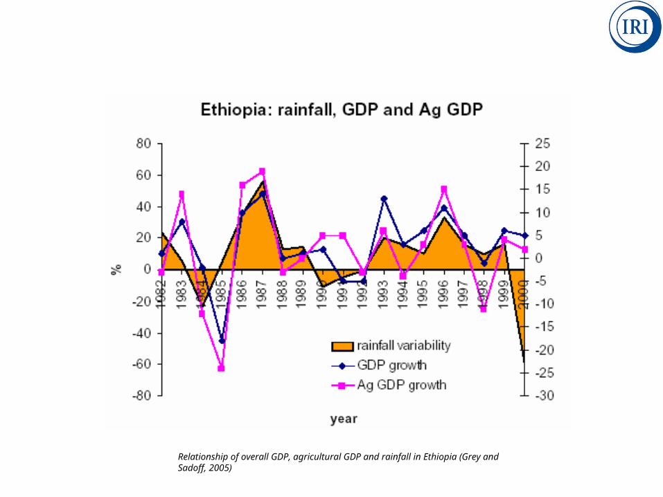
Relationship of overall GDP, agricultural GDP and rainfall in Ethiopia (Grey and Sadoff, 2005)

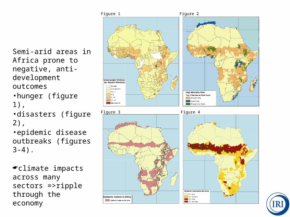
Semi-arid areas in Africa prone to negative, anti-development outcomes •hunger (figure 1), •disasters (figure 2), •epidemic disease outbreaks (figures 3-4).

climate impacts across many sectors =>ripple through the economy

Figure 1 Figure 2

Figure 3 Figure 4

Climate PredictionClimate Prediction

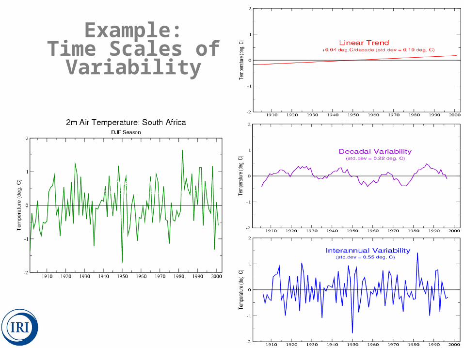
Example:Time Scales of

Variability

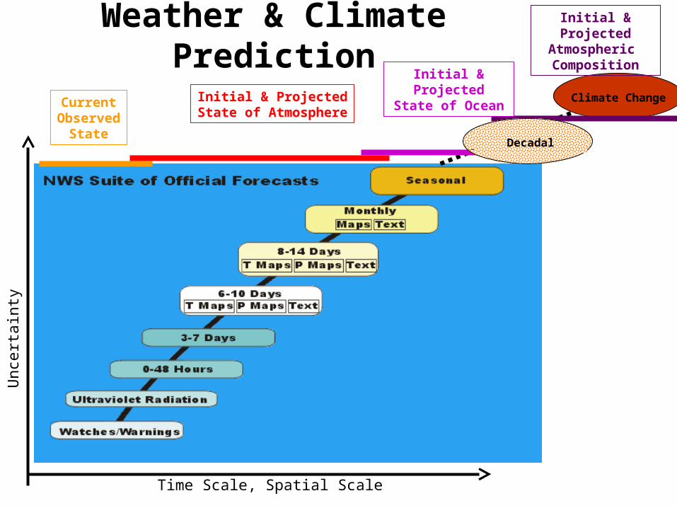
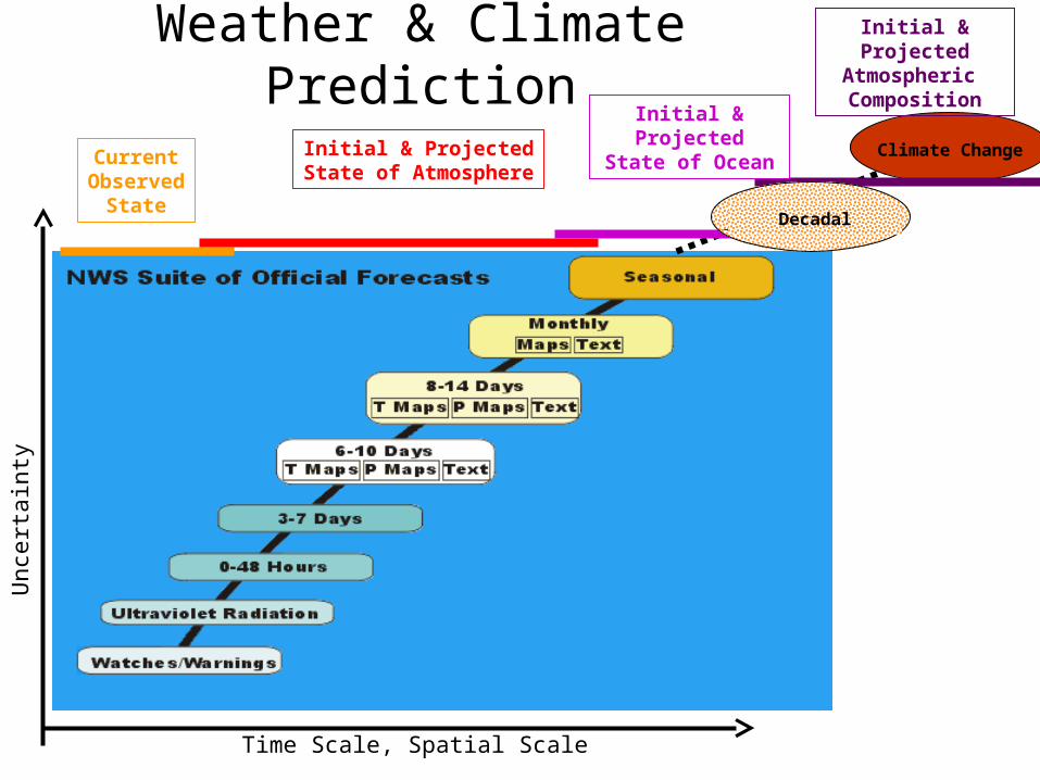
Weather & Climate Prediction

Climate Change

Unce

rtain

ty

Time Scale, Spatial Scale

CurrentObserved

State

Initial & ProjectedState of Atmosphere

Initial & Projected

Atmospheric Composition

Decadal

Initial & Projected

State of Ocean

Basis of Seasonal Climate Prediction:

Changes in boundary conditions, such as SST and land surface characteristics, can influence the characteristics of weather (e.g. strength or persistence/absence), and thus influence the seasonal climate.

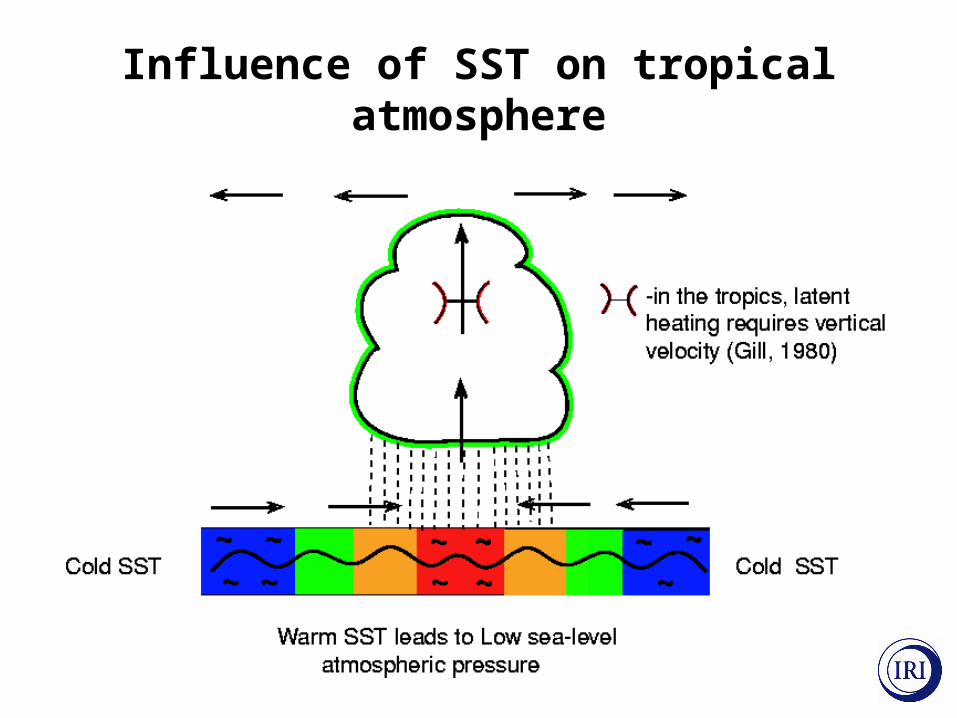
Influence of SST on tropical atmosphere

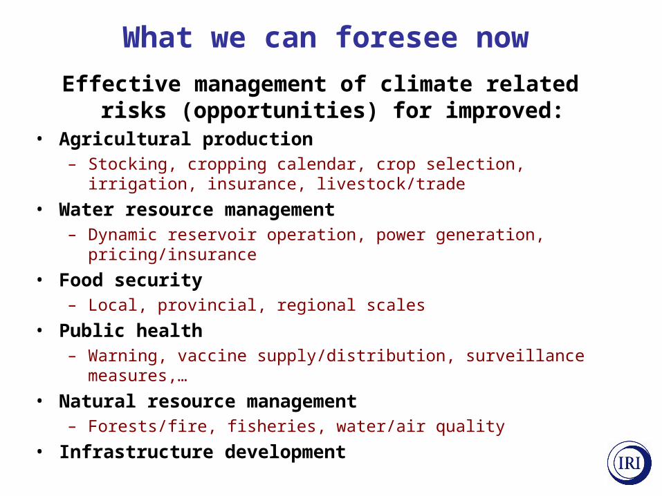
What we can foresee now

Effective management of climate related risks (opportunities) for improved:

• Agricultural production– Stocking, cropping calendar, crop selection, irrigation, insurance,

livestock/trade

• Water resource management– Dynamic reservoir operation, power generation, pricing/insurance

• Food security– Local, provincial, regional scales

• Public health– Warning, vaccine supply/distribution, surveillance measures,…

• Natural resource management– Forests/fire, fisheries, water/air quality

• Infrastructure development

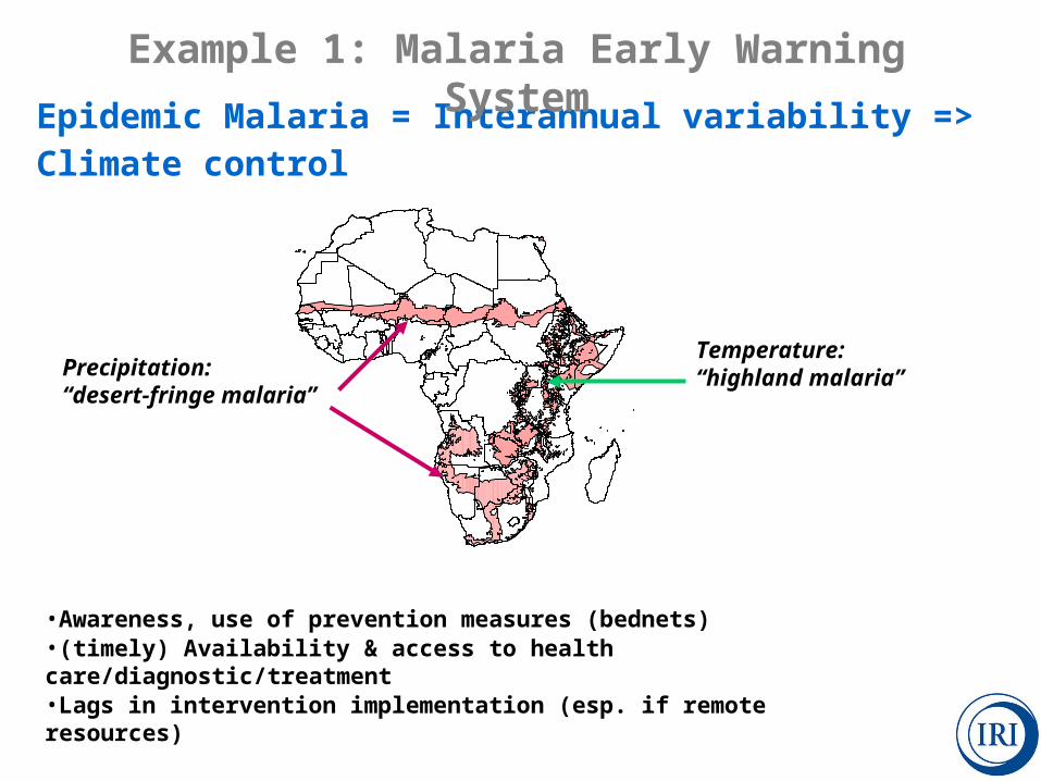
Epidemic Malaria = Interannual variability => Climate control

Example 1: Malaria Early Warning System

Temperature: “highland malaria”Precipitation:

“desert-fringe malaria”

•Awareness, use of prevention measures (bednets)•(timely) Availability & access to health care/diagnostic/treatment•Lags in intervention implementation (esp. if remote resources)

Month

JULMAYMARJANNOVSEP

200

100

0

Rainfall (mm)

Malaria incidence

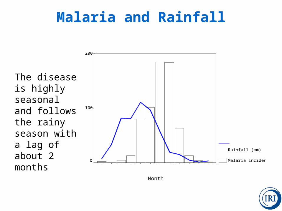
The disease is highly seasonal and follows the rainy season with a lag of about 2 months

Malaria and Rainfall

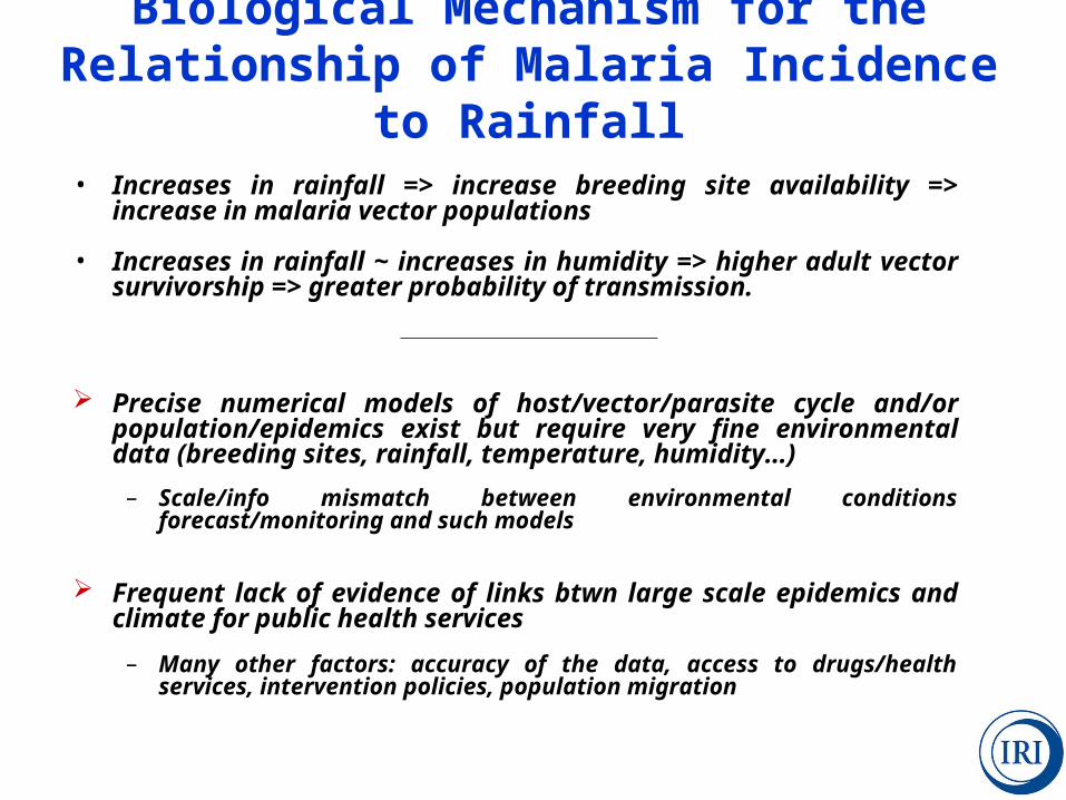
• Increases in rainfall => increase breeding site availability => increase in malaria vector populations

• Increases in rainfall ~ increases in humidity => higher adult vector survivorship => greater probability of transmission.

Precise numerical models of host/vector/parasite cycle and/or population/epidemics exist but require very fine environmental data (breeding sites, rainfall, temperature, humidity…)

– Scale/info mismatch between environmental conditions forecast/monitoring and such models

Frequent lack of evidence of links btwn large scale epidemics and climate for public health services

– Many other factors: accuracy of the data, access to drugs/health services, intervention policies, population migration

Biological Mechanism for the Relationship of Malaria Incidence to Rainfall

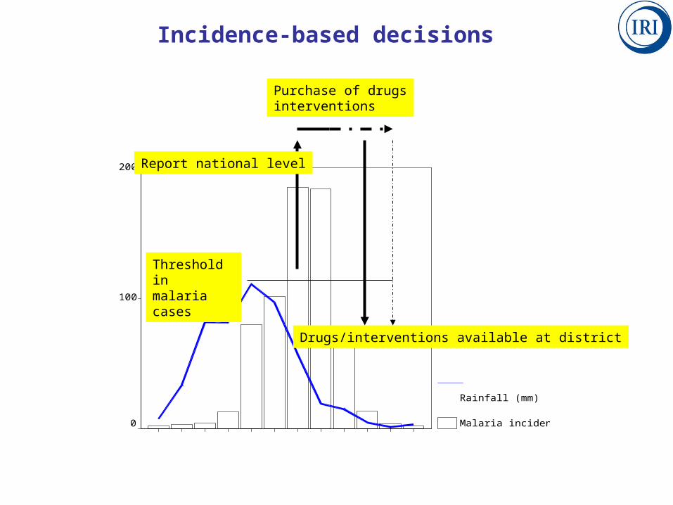
Incidence-based decisions

Month

JULMAYMARJANNOVSEP

200

100

0

Rainfall (mm)

Malaria incidence

Threshold in malaria cases

Report national level

Purchase of drugsinterventions

Drugs/interventions available at district

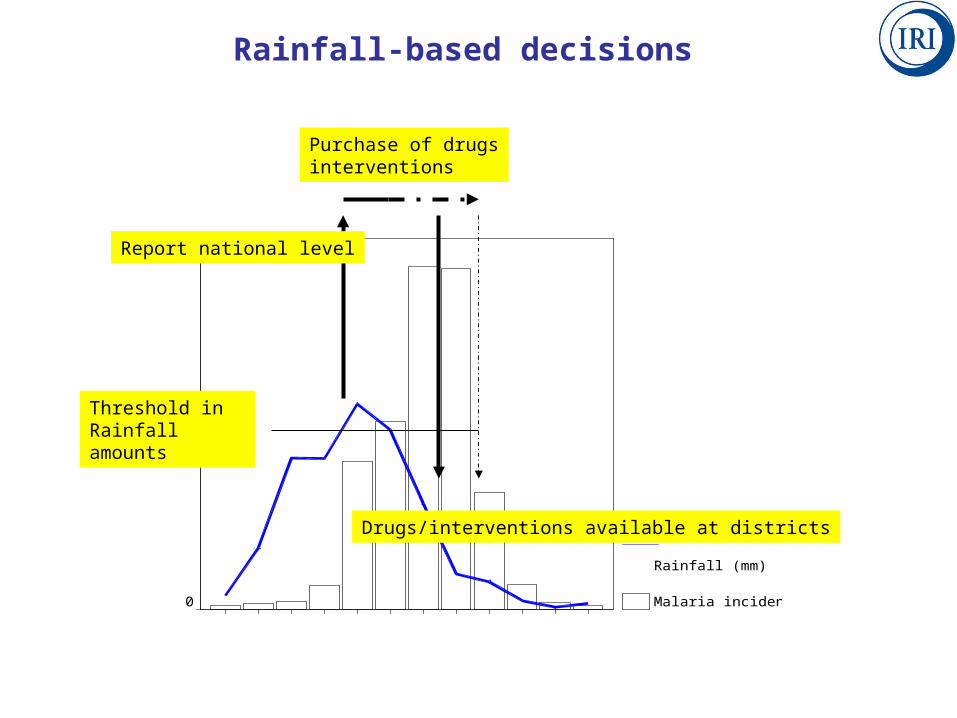
Rainfall-based decisions

Month

JULMAYMARJANNOVSEP

200

100

0

Rainfall (mm)

Malaria incidence

Threshold in Rainfall amounts

Drugs/interventions available at districts

Report national level

Purchase of drugsinterventions

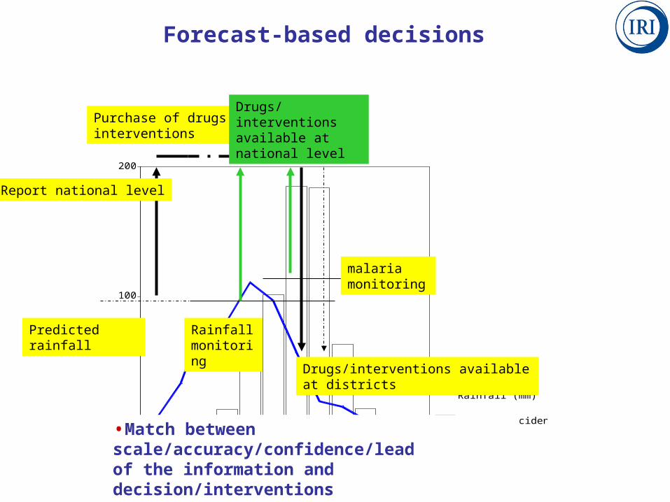
Forecast-based decisions

Month

JULMAYMARJANNOVSEP

200

100

0

Rainfall (mm)

Malaria incidence

Drugs/interventions available at districts

Report national level

Purchase of drugsinterventions

Predicted rainfall

malaria monitoring

Rainfall monitoring

Drugs/interventions available at national level

•Match between scale/accuracy/confidence/lead of the information and decision/interventions•More effective use of limited resources•Interactions with end-users are crucial

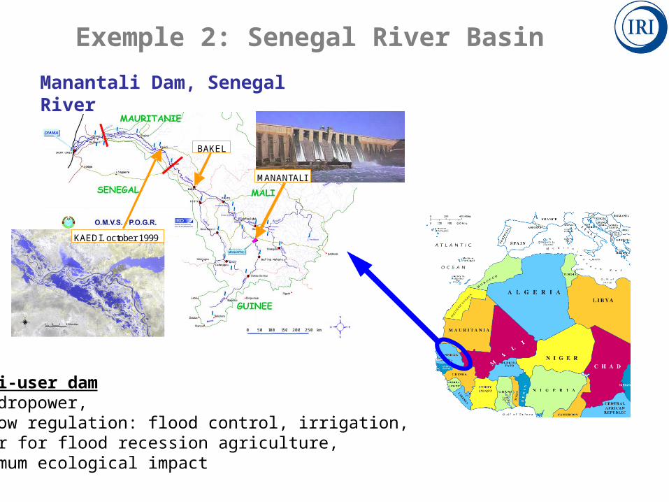
Manantali Dam, Senegal River

MANANTALI

KAEDI, october 1999

BAKEL

0 50 100 150 200 250 km

Multi-user dam• Hydropower, • flow regulation: flood control, irrigation,water for flood recession agriculture,minimum ecological impact

Exemple 2: Senegal River Basin

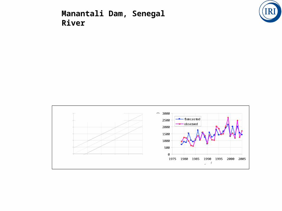
Manantali Dam, Senegal River

0

500

1000

1500

2000

2500

3000

1975 1980 1985 1990 1995 2000 2005

forecasted

observed

year

natu

ral dis

charg

e (

m3/s

)

R2 = 0.6507

0

500

1000

1500

2000

2500

3000

0 500 1000 1500 2000 2500

1979-2000 (calibration)2000-2005 (validation)80% interval90% interval

Qd = f (V1,…V5) : forecasted natural discharge (m3/s)

observ

ed n

atu

ral dis

charg

e (

m3/s

)

August 20 – reservoir management decision for water release for traditional agriculture Sept-Oct, given electricity and irrigation demands Sept-July

Management strategy using Aug-Oct seasonal forecast made at Meteo-France end of July

=> Forecast water stock in the reservoir at the end of the monsoon season

Seasonal ForecastsSeasonal Forecasts

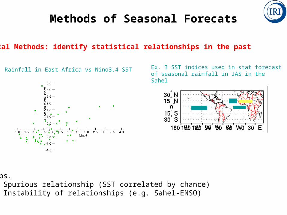
Methods of Seasonal Forecats

Statistical Methods: identify statistical relationships in the past

Ex. Rainfall in East Africa vs Nino3.4 SST Ex. 3 SST indices used in stat forecast of seasonal rainfall in JAS in the Sahel

Pbs. • Spurious relationship (SST correlated by chance)• Instability of relationships (e.g. Sahel-ENSO)

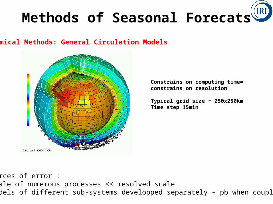
Sources of error :•Scale of numerous processes << resolved scale•Models of different sub-systems developped separately – pb when coupling

Constrains on computing time= constrains on resolution

Typical grid size ~ 250x250kmTime step 15min

Dynamical Methods: General Circulation Models

Methods of Seasonal Forecats

Weather & Climate Prediction

Climate Change

Unce

rtain

ty

Time Scale, Spatial Scale

CurrentObserved

State

Initial & ProjectedState of Atmosphere

Initial & Projected

Atmospheric Composition

Decadal

Initial & Projected

State of Ocean

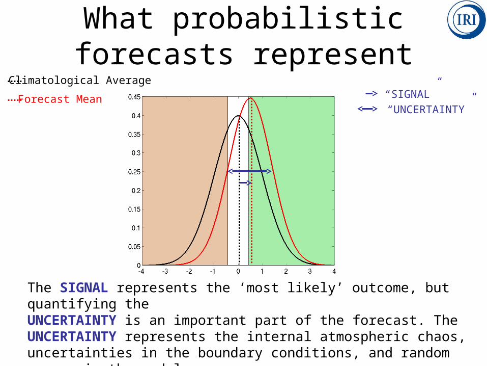
What probabilistic forecasts represent

Climatological Average

Forecast Mean “SIGNAL”

The SIGNAL represents the ‘most likely’ outcome, but quantifying theUNCERTAINTY is an important part of the forecast. The UNCERTAINTY represents the internal atmospheric chaos, uncertainties in the boundary conditions, and random errors in the models.

“UNCERTAINTY”

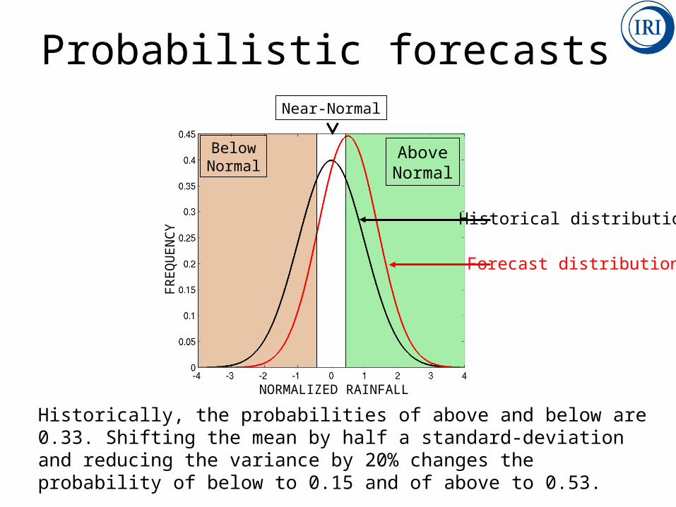
BelowNormal

AboveNormal

Historically, the probabilities of above and below are 0.33. Shifting the mean by half a standard-deviation and reducing the variance by 20% changes the probability of below to 0.15 and of above to 0.53.

Historical distribution

Forecast distribution

Probabilistic forecasts Near-Normal

NORMALIZED RAINFALL

FR

EQ

UE

NC

Y

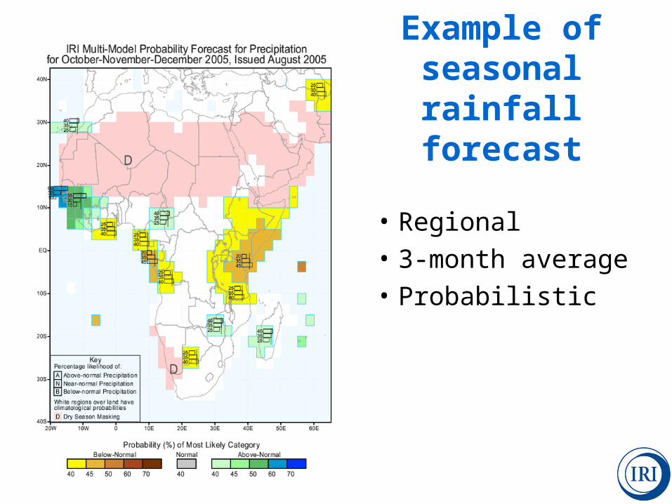
Example of seasonal

rainfall forecast

• Regional

• 3-month average

• Probabilistic

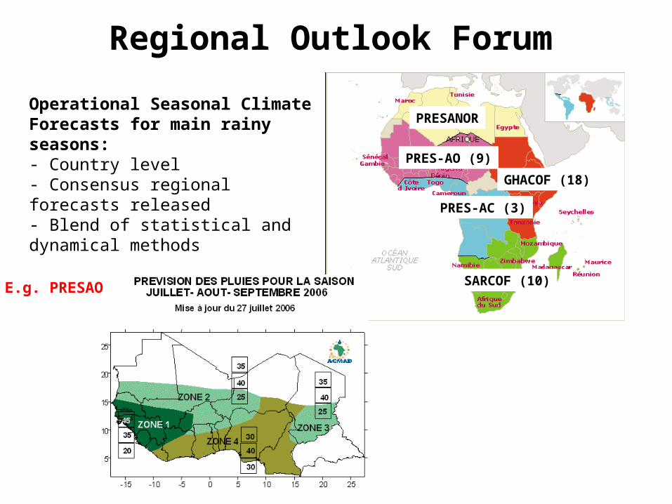
PRES-AO (9)

GHACOF (18)

PRES-AC (3)

SARCOF (10)

PRESANOR

Regional Outlook Forum

Operational Seasonal Climate Forecasts for main rainy seasons:- Country level- Consensus regional forecasts released- Blend of statistical and dynamical methods

E.g. PRESAO

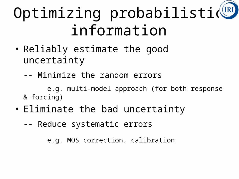
Optimizing probabilistic information

• Reliably estimate the good uncertainty

-- Minimize the random errors

e.g. multi-model approach (for both response & forcing)

• Eliminate the bad uncertainty

-- Reduce systematic errors

e.g. MOS correction, calibration

Use of Ocean DataUse of Ocean Data

30

12

30

24

12

24

24

24

10

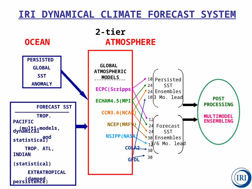
FORECAST SST

TROP. PACIFIC (multi-models, dynamical and statistical)

TROP. ATL, INDIAN (statistical)

EXTRATROPICAL (damped persistence)

GLOBAL ATMOSPHERIC

MODELS

ECPC(Scripps)

ECHAM4.5(MPI)

CCM3.6(NCAR)

NCEP(MRF9)

NSIPP(NASA)

COLA2

GFDL

ForecastSST

Ensembles3/6 Mo. lead

PersistedSST

Ensembles3 Mo. lead

IRI DYNAMICAL CLIMATE FORECAST SYSTEM

POSTPROCESSING

MULTIMODELENSEMBLING

PERSISTED

GLOBAL

SST

ANOMALY

2-tier OCEAN ATMOSPHERE

30

10

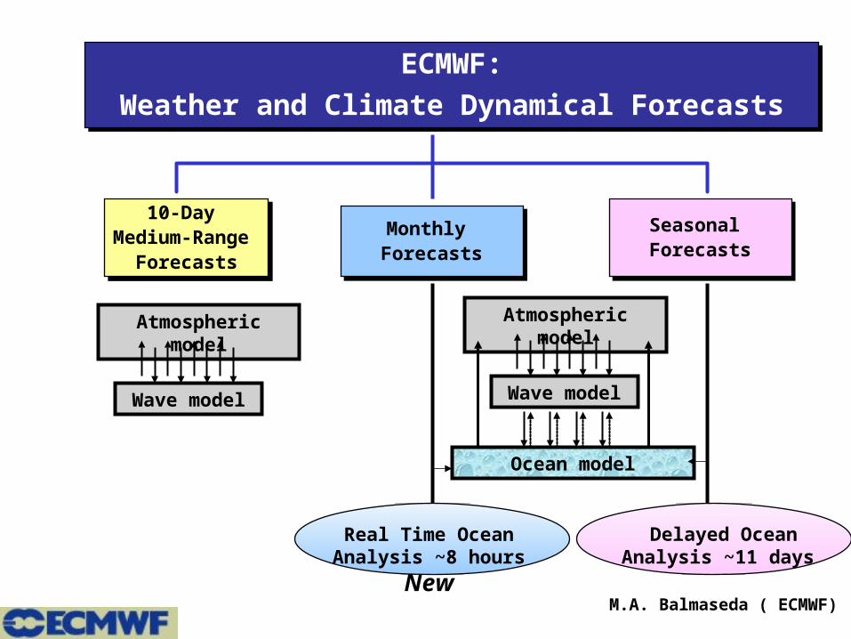
Delayed Ocean Analysis ~11 days

Real Time Ocean Analysis ~8 hours

New

ECMWF:

Weather and Climate Dynamical Forecasts

ECMWF:

Weather and Climate Dynamical Forecasts

10-Day Medium-Range

Forecasts

10-Day Medium-Range

Forecasts

Seasonal Forecasts

Seasonal Forecasts

Monthly Forecasts

Monthly Forecasts

Atmospheric model

Wave model

Ocean model

Atmospheric model

Wave model

M.A. Balmaseda ( ECMWF)

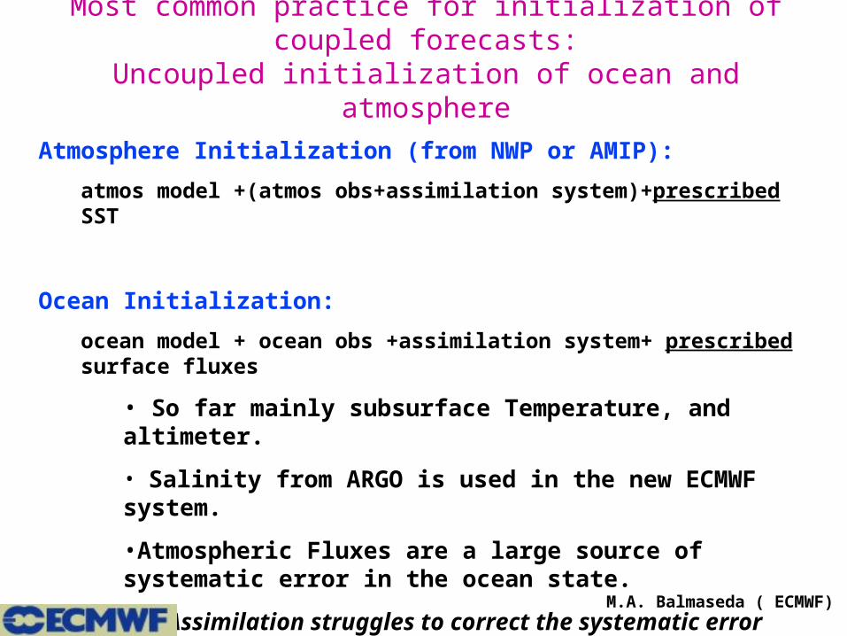
Most common practice for initialization of coupled forecasts:Uncoupled initialization of ocean and atmosphere

Atmosphere Initialization (from NWP or AMIP):

atmos model +(atmos obs+assimilation system)+prescribed SST

Ocean Initialization:

ocean model + ocean obs +assimilation system+ prescribed surface fluxes

• So far mainly subsurface Temperature, and altimeter.

• Salinity from ARGO is used in the new ECMWF system.

•Atmospheric Fluxes are a large source of systematic error in the ocean state.

•Data Assimilation struggles to correct the systematic error

M.A. Balmaseda ( ECMWF)

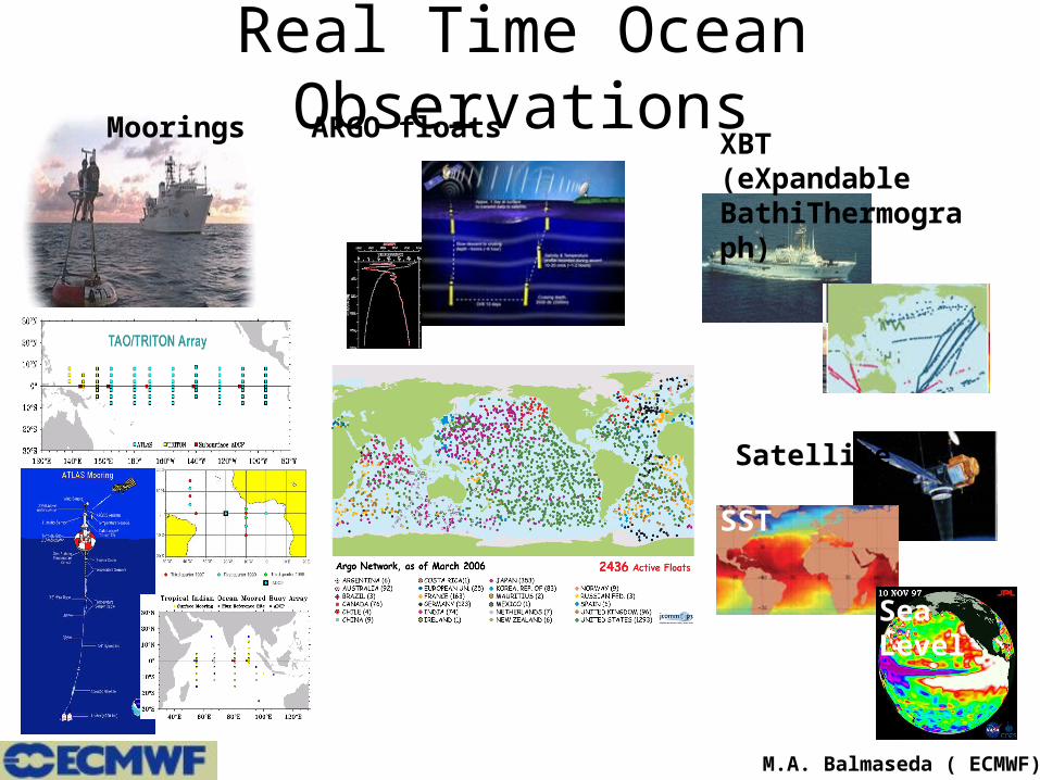
Real Time Ocean ObservationsARGO floats

XBT (eXpandable BathiThermograph)

Moorings

Satellite

SST

Sea Level

M.A. Balmaseda ( ECMWF)

60°S 60°S

30°S30°S

0° 0°

30°N30°N

60°N 60°N

60°E

60°E

120°E

120°E

180°

180°

120°W

120°W

60°W

60°W

0°

0°

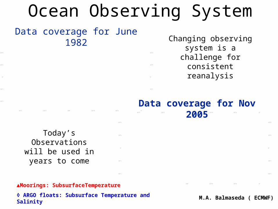
X B T p r o b e s : 9 3 7 6 p r o f i l e sOBSERVATION MONITORING Changing observing

system is a challenge for consistent reanalysis

Today’s Observations will be used in years

to come

60°S 60°S

30°S30°S

0° 0°

30°N30°N

60°N 60°N

60°E

60°E

120°E

120°E

180°

180°

120°W

120°W

60°W

60°W

0°

0°▲Moorings: SubsurfaceTemperature

◊ ARGO floats: Subsurface Temperature and Salinity

+ XBT : Subsurface Temperature

Data coverage for June 1982

Ocean Observing System

M.A. Balmaseda ( ECMWF)

Data coverage for Nov 2005

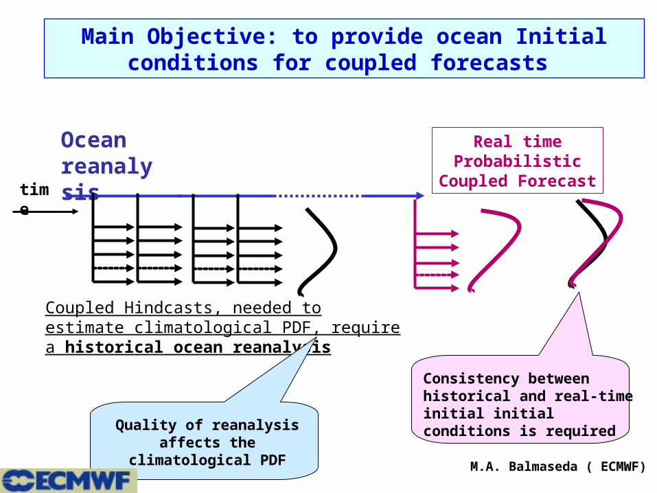
Coupled Hindcasts, needed to estimate climatological PDF, require a historical ocean reanalysis

Real time Probabilistic Coupled

Forecasttime

Ocean reanalysis

Quality of reanalysis affects the climatological

PDF

Consistency between historical and real-time initial initial conditions is required

Main Objective: to provide ocean Initial conditions for coupled forecasts

M.A. Balmaseda ( ECMWF)

Importance of ARGO DataImportance of ARGO Data

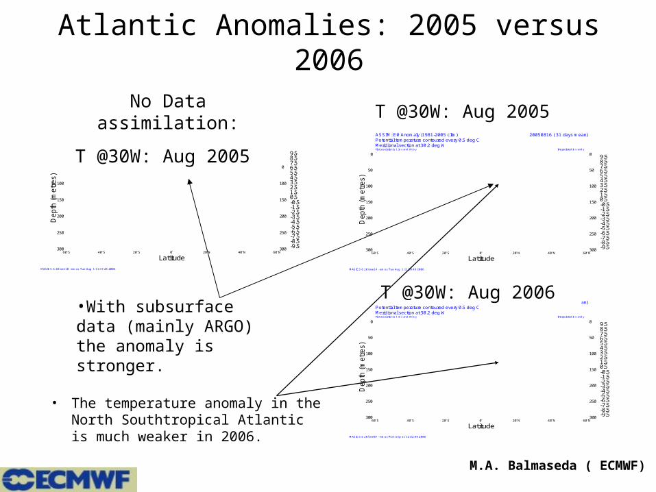
Atlantic Anomalies: 2005 versus 2006

• The temperature anomaly in the North Southtropical Atlantic is much weaker in 2006.

60OS 40OS 20OS 0O 20ON 40ON 60ON

Latitude

300

250

200

150

100

50

0

Depth

(m

etr

es)

300

250

200

150

100

50

0Plot resolution is 1 in x and 10 in y

Meridional section at 30.2 deg WPotential temperature contoured every 0.5 deg CASSIM: E0 Anomaly (1981-2005 clim)

Interpolated in x and y

20050816 ( 31 days mean)

-9.5-8.5-7.5-6.5-5.5-4.5-3.5-2.5-1.5-0.50.51.52.53.54.55.56.57.58.59.5

MAGICS 6.10 bee14 - emos Tue Aug 1 11:20:49 2006

60OS 40OS 20OS 0O 20ON 40ON 60ON

Latitude

300

250

200

150

100

50

0

Depth

(m

etr

es)

300

250

200

150

100

50

0Plot resolution is 1 in x and 10 in y

Meridional section at 30.2 deg WPotential temperature contoured every 0.5 deg CS3 ASSIM (E0): Anomaly (1981-2005 clim)

Interpolated in x and y

20060816 ( 31 days mean)

-9.5-8.5-7.5-6.5-5.5-4.5-3.5-2.5-1.5-0.50.51.52.53.54.55.56.57.58.59.5

MAGICS 6.10 bee07 - emos Mon Sep 11 12:52:49 2006

T @30W: Aug 2005

T @30W: Aug 2006

60OS 40OS 20OS 0O 20ON 40ON 60ON

Latitude

300

250

200

150

100

50

0

Depth

(m

etr

es)

300

250

200

150

100

50

0Plot resolution is 1 in x and 10 in yMeridional section at 30.2 deg WPotential temperature contoured every 0.5 deg CCONTROL: E0 Anomaly (1981-2005 clim)

Interpolated in x and y

20050816 ( 31 days mean)

-9.5-8.5-7.5-6.5-5.5-4.5-3.5-2.5-1.5-0.50.51.52.53.54.55.56.57.58.59.5

MAGICS 6.10 bee10 - emos Tue Aug 1 11:17:45 2006

No Data assimilation:

T @30W: Aug 2005

•With subsurface data (mainly ARGO) the anomaly is stronger.

M.A. Balmaseda ( ECMWF)

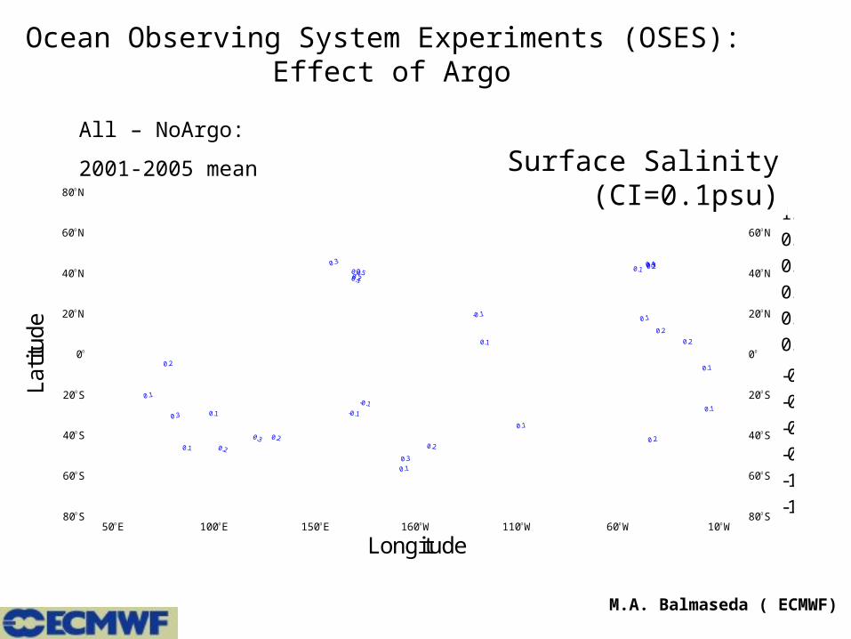
Ocean Observing System Experiments (OSES): Effect of Argo

50OE 100OE 150OE 160OW 110OW 60OW 10OW

Longitude

80OS

60OS

40OS

20OS

0O

20ON

40ON

60ON

80ON

Latit

ude

80OS

60OS

40OS

20OS

0O

20ON

40ON

60ON

80ON

Plot resolution is 1.4063 in x and 1 in yHorizontal section at 5.0 metres depthSalinity contoured every 0.1 psu: erfk - esrz

Interpolated in y 0 ( 5 year mean)

difference from20060101 ( 5 year mean)

-0.1-0.1

-0.1

0.1

0.1

0.1

0.10.1

0.1

0.1

0.1

0.1

0.1

0.1

0.2

0.2 0.20.2

0.2

0.2

0.2

0.2

0.2

0.3

0.3

0.3

0.30.30.4

0.40.5

-1.2

-1

-0.8

-0.6

-0.4

-0.2

0.1

0.3

0.5

0.7

0.9

1.1

MAGICS 6.9.1 hyrokkin - neh Tue Aug 8 17:04:33 2006

Surface Salinity (CI=0.1psu)All – NoArgo:

2001-2005 mean

M.A. Balmaseda ( ECMWF)

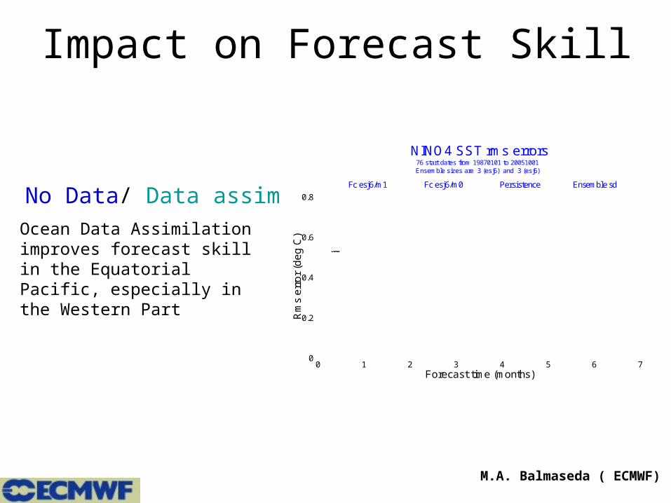
Impact on Forecast Skill

0 1 2 3 4 5 6 7Forecast time (months)

0.4

0.5

0.6

0.7

0.8

0.9

1

An

om

aly

co

rre

latio

n

wrt NCEP adjusted OIv2 1971-2000 climatology

NINO4 SST anomaly correlation

0 1 2 3 4 5 6 7Forecast time (months)

0

0.2

0.4

0.6

0.8

Rm

s e

rro

r (d

eg

C)

Ensemble sizes are 3 (esj6) and 3 (esj6) 76 start dates from 19870101 to 20051001

NINO4 SST rms errors

Fc esj6/m1 Fc esj6/m0 Persistence Ensemble sd

MAGICS 6.10 hyrokkin - neh Thu Sep 7 19:11:46 2006

Ocean Data Assimilation improves forecast skill in the Equatorial Pacific, especially in the Western Part

No Data/ Data assim

M.A. Balmaseda ( ECMWF)

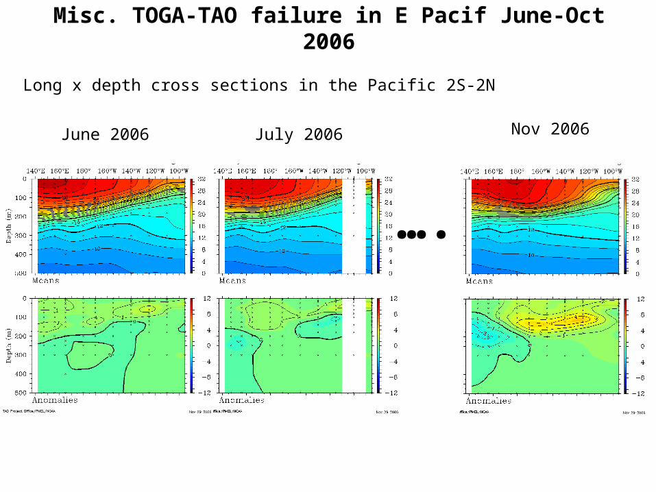
Misc. TOGA-TAO failure in E Pacif June-Oct 2006

June 2006

Long x depth cross sections in the Pacific 2S-2N

July 2006 Nov 2006

….

Research!Research!

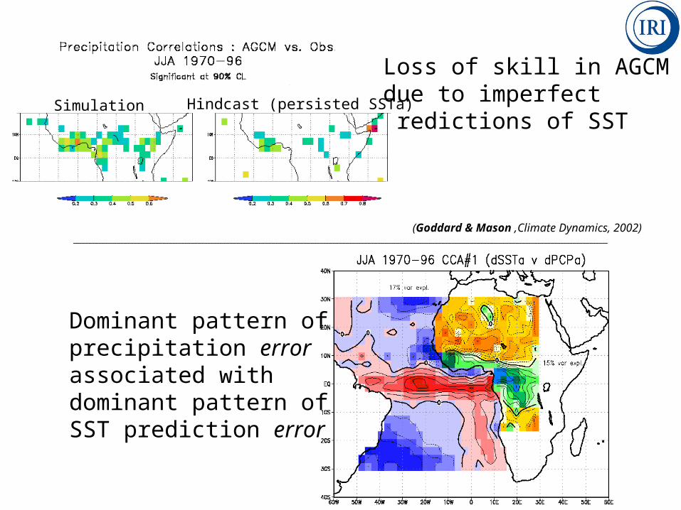
Loss of skill in AGCMdue to imperfect predictions of SST

Dominant pattern ofprecipitation errorassociated withdominant pattern ofSST prediction error

(Goddard & Mason ,Climate Dynamics, 2002)

Simulation Hindcast (persisted SSTa)

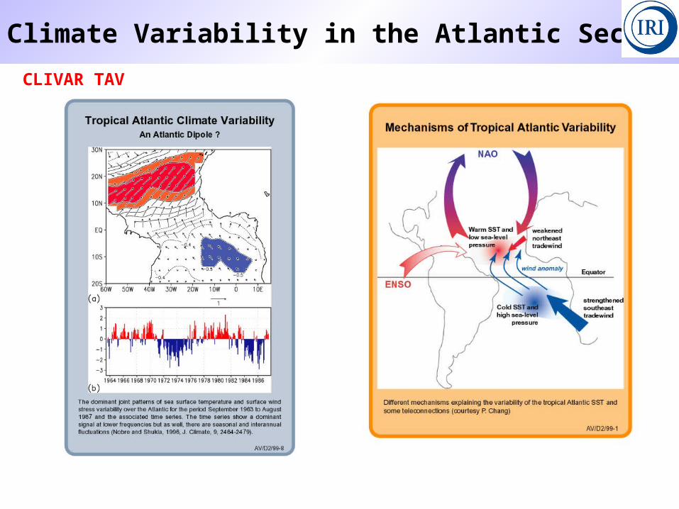
Climate Variability in the Atlantic Sector

CLIVAR TAV

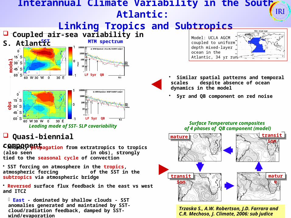
Interannual Climate Variability in the South Atlantic: Linking Tropics and Subtropics

Trzaska S., A.W. Robertson, J.D. Farrara and C.R. Mechoso, J. Climate, 2006: sub judice

maturemature

transitiontransition

transitiontransition

maturemature

Model: UCLA AGCM coupled to uniform depth mixed-layer ocean in the Atlantic, 34 yr run

Similar spatial patterns and temporal scales despite absence of ocean dynamics in the model

5yr and QB component on red noise

Quasi-biennial component Anomaly propagation from extratropics to tropics (also seen

in obs), strongly tied to the seasonal cycle of convection

SST forcing on atmosphere in the tropics, atmospheric forcing of the SST in the subtropics via atmospheric bridge

Reversed surface flux feedback in the east vs west and ITCZ

East - dominated by shallow clouds - SST anomalies generated and maintained by SST- cloud/radiation feedback, damped by SST- wind/evaporation

West and ITCZ - deep convection - SST anomalies generated and maintained by SST- wind/evaporation, damped by SST- cloud/radiation feedback

Surface Temperature composites of 4 phases of QB component (model)

LF 5yr QB

ob

s

SST MTM spectrum

LF 5yr QB

mo

de

l

Coupled air-sea variability in S. Atlantic

Leading mode of SST- SLP covariability

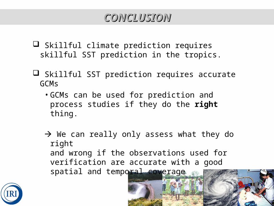
CONCLUSIONCONCLUSION

Skillful climate prediction requires skillful SST prediction in the tropics.

Skillful SST prediction requires accurate GCMs• GCMs can be used for prediction and process

studies if they do the right thing.

We can really only assess what they do rightand wrong if the observations used for verification are accurate with a good spatial and temporal coverage

Climate InformationClimate Information

http://iri.columbia.edu•Data Library: numerous data incl. seasonal forecast, mapping &analysis tools•Tutorials and Manuals•Climate Prediction Tool