Turbidity front dynamics of the Musi Banyuasin Estuary

AACL Bioflux, 2021, Volume 14, Issue 1.

http://www.bioflux.com.ro/aacl 1

Turbidity front dynamics of the Musi Banyuasin

Estuary using numerical model and Landsat 8

satellite 1Septy Heltria, 2I Wayan Nurjaya, 2Jonson L. Gaol

1 Marine Science Postgraduate, Faculty of Fisheries and Marine Science, IPB University,

Darmaga Bogor, West Java, Indonesia; 2 Department of Marine Science and Technology,

Faculty of Fisheries and Marine Science, IPB University, Darmaga Bogor, West Java,

Indonesia. Corresponding author: I. W. Nurjaya, [email protected]

Abstract. Rivers bring organic and non-organic materials into the estuary, causing changes in the turbidity of the water. The hydrodynamic processes cause fresh water with different turbidity to be distributed towards the estuary, where it is trapped due to differences in the density of freshwater and seawater, forming a turbidity front (TF). The TF can be a trap of contaminated materials. However, it can be a reference for fishing areas due to the accumulation of nutrients. The study aims to analyze the hydrodynamic conditions and their effects on distribution patterns and turbidity front positions using 2D numerical models and remote sensing at Musi Banyuasin Estuary (MBE). Tides are dominant in controlling the flow and can determine the position of the TF. The verification value of the average relative error (MRE) of the model and in situ data is 30.74%. Landsat image analysis confirmed by the turbidity model shows that the TF formed in the turbidity range of 40-50 FTU. Model simulation results and images were directly proportional; the furthest distance where TF formed was at the lowest ebb in neap tide, 14.87 km (model) and 15.56 km (satellite). The correlation between satellite data and the turbidity model was validated with r≥0.5. Key Words: brackish water, hydrodynamic model, satellite imagery, simulation.

Introduction. The estuary is a transitional area where organic and non-organic

materials from various sources are trapped before entering the sea. The accumulation of

these materials indirectly causes the waters to become turbid and spread to the mouth of

the estuary. Turbidity shows the level of brightness of the water measured by the

amount of light scattered by the material in the water (Derisio et al 2014; Nurjaya et al

2019).

The turbidity distribution is influenced by differences in the mass density of

freshwater and seawater, forming a turbidity front (TF). The TF is rich in nutrients that

are brought from upstream. The nutrients trigger the growth of phytoplankton and

increase productivity (Ge et al 2020). The position of the TF in the estuary's mouth is

interestingly to observe, because it can be an indicator of fishing grounds. This is also

supported by the existence of fish migration routes from sea to river or vice versa (Blaber

1997).

Musi Banyuasin Estuary is a large estuary where accumulations of organic and

non-organic inputs occur from rivers in South Sumatra, specifically the Banyuasin River,

Telang River, Musi River, and Upang River. The activity around the River is very high. The

Central Statistics Agency (BPS) of South Sumatra (2016) recorded agriculture activities

in Banyuasin and Musi Banyuasin Regencies on 298.231 ha and 500.212 ha, respectively.

Temporary storages of coal are found along the Banyuasin River (Purwiyanto 2015; Putri

et al 2016) and the domestic and industrial waste disposal in the Musi River located in

the Palembang city is very active. These activities indirectly change the turbidity of the

waters.

The hydrodynamic process that describes the pattern of water mass flow in the

Musi Estuary and the Banyuasin Estuary was studied. The research results of Surbakti



(2012) and Nurisman et al (2012) show that the tidal type in the Musi River Estuary is

diurnal, and the flow was dominated by tidal currents with a speed of 10.1 cm s-1. 2D

hydrodynamic models and salinity distribution patterns were studied by Sari et al (2013)

in the Musi Estuary. Salinity ranged from 0.9 to 23.9‰. The wind does not have a

significant effect on the distribution of salinity. The tidal type at the Banyuasin Estuary is

diurnal, but the tidal current type is mixed, prevailing diurnal with a maximum current

speed of 0.34 m s-1 and a tidal current of 0.35 m s-1 (Simatupang et al 2016). There is

little information about the pattern of distribution and position of the TF due to river

activity in the Musi Banyuasin estuary.

This study aims to analyze the distribution patterns and determine the TF position

using the numerical model approach and remote sensing during spring and neap

conditions in the Musi Banyuasin estuary. This study can provide information related to

the influence of hydrodynamics to turbidity distribution in determining TF position.

Material and Method

Description of the study sites. The study was conducted at the Musi Banyuasin

estuary, where 4 rivers drain, namely the Musi River, Telang River, Upang River, and

Banyuasin River (Figure 1). Telang and Upang rivers are part of the Musi River. Telang

River drains into the Musi estuary, where the Payung Island affects the flow before

entering or exiting the estuary. The Upang River forms the Upang Delta in the Musi River.

Data was collected between 1 and 10 September 2016.

Figure 1. Research location at the Musi River Estuary, East Coast of South Sumatra,

Indonesia.

Collection of data. Salinity, temperature, density, and turbidity in Telang River and

Musi River were collected in low tide condition using a CTD (Conductivity Temperature

Depth) Sensor at 21 stations (Figure 1). Data in the Upang River were obtained from

Sinaga et al (2019) and the Banyuasin River from Surbakti et al (2014) and Suteja et al

(2019). Discharge data from the Musi River (M4) and Telang River (M3) were obtained



using a current meter. Tidal data in mid-estuary Musi (M2) and the mouth of Musi

estuary (M1) were obtained for model verification.

Numerical model processing. The larger model consists of hydrodynamic models, 2D

salinity distribution and 2D transport (turbidity) models that are processed using MIKE 21

Software. Hydrodynamic models describe the flow conditions in the Banyuasin Musi

Estuary, which were simulated using bathymetry, tidal, and river discharge data.

Furthermore, the transport model (turbidity) was built to determine the turbidity's

distribution, so that the TF position could be determined. The model was simulated for 21

days to describe the condition of spring and neap tide with the configuration of the model

(Table 1).

Table 1

Configuration of hydrodynamic and turbidity models

Parameter Application of simulation

Model

characteristics 2D

Simulation time

Number of steps

Time step interval

Simulation period

6048

30

01/09/2016 01:00:00 –

22/09/2016 23:00:00

Area Maximum element area

Angle mesh

0.0005 (deg)2

26 (deg)

Grid Origin (in Geographic WGS 84) 105.081E -2.105S

Mesh boundary

1. Bathymetry data PUSHIDROSAL 2015

2. Bathymetry data BIG 2015

3. Field tidal data September 2016

Discharge

Telang river

Musi river

Upang river

142.6 m3 s-1

202.15 m3 s-1

211.7 m3 s-1

Tidal excursion. The tidal excursion is a horizontal distance that can describe the

movement of particles or pollutants from the river mouth to the sea in the tidal cycle

(Zhen-Gang 2008). It can be determined using the following equation (Savenije 2012):

E=1.08

Where: E is a tidal excursion; V0 is the tidal velocity amplitude; T is the tidal period, the

period used was based on the dominant harmonic component in the study area.

Image data processing. Image data used is Landsat 8 OLI imagery with a spatial

resolution of 30x30 m, which can be downloaded freely on its website page

(https://earthexplorer.usgs.gov/). TF detection used imagery on the acquisition date of

20 July 2017 (neap tide) and 12 August 2018 (spring tide). Neap and spring tides were

determined based on moon position, neap occurring during the first and third quarter

moon and spring tide occurring during new and full moon. The turbidity concentration of

the satellite uses the reflectance value of the red band (band 4) (Nechad et al 2009), as

in the following equation:

T =

Where: AT and C are calibration coefficients that depend on wavelength. The AT

coefficient was obtained by a non-linear least-square regression analysis using in situ

measurements of T and ρw. C was calibrated using “standard” inherent optical properties



(IOPs) as described in Nechad et al (2010); ρw is the reflectance value; 𝜆 is the

wavelength. The reflectance value on the image used was higher than 0.07, using the

859 nm band, categorized as having a moderate to high turbidity concentration (Dogliotti

et al 2015). The calibration coefficients of AT and C (FNU) for 859 nm were obtained from

Nechad et al (2010) and Dogliotti et al (2011). The resulting turbidity distribution was

grouped in 5 classes with an Isoturbid contour range (lines in the same turbidity range)

for 25 FTU.

Statistical analysis. All 2D model data such as hydrodynamics, salinity distribution and

turbidity transport were analyzed with the MIKE 21 software. The model verification

method used is the verification of the average relative error (mean relative error - MRE).

If the MRE values is lower than 50%, the model is accepted, and if the MRE is higher

than 50%, the simulation should be repeated (Zaman & Syafrudin 2007). The correlation

between model and image data was analyzed with a linear regression model.

Results and Discussion. Musi Banyuasin estuary is a meeting place of four rivers,

namely Upang River, Musi River, Telang River, and Banyuasin River, which directly faces

the Bangka Strait. The flow of rivers and tides influences the dynamics of water mass in

the estuary. The main flow of discharge originates from the Musi estuary, which has

three branches, namely the Telang River, the Musi River, and the Upang River.

Water mass characteristics are illustrated through the vertical distribution of

salinity and temperature (Figure 2). The salinity of Telang River and Musi River reaches

6.4 and 4.5 PSU, respectively, at the boundary. The difference in salinity value of 2 PSU

is thought to be influenced by the existence of Payung Island, in front of the other river

flows before estuary. The temperature of the 2 rivers is almost the same, namely 29.5⁰C

at the surface, and 30⁰C in the water column. Figure 2 shows the mixing of water

masses, causing salinity stratification so that the estuarine water is partially mix. The

distribution of salinity and water temperature of the Upang river was illustrated by the

study of Sinaga et al (2019) and in the Banyuasin river by Suteja et al (2019).

Figure 2. Distribution of temperature and salinity; a - from the Telang River to the Musi

Estuary; b - from the Musi River to the Musi Estuary.

Musi Banyuasin Estuary has a diurnal type of tide with the Formzahl number 3.06, which

is one high and low tide occurring in one day, according to the results of the previous



studies (Radjwane et al 2018). The tidal range at Muara Musi Banyuasin at the neap tide

is 1.07 to 2.03 m during spring tide (Figure 3). The hydrodynamic model validation

(Figure 4) has the mean relative error (MRE) verification value of 30.74%, which means

that the model results are sufficient to describe the similarity of hydrodynamic conditions

in the study area.

The in situ data collection in estuary's mouth shows two peaks at high tide. The

masses of seawater and freshwater enter simultaneously and cause an accumulation of

water masses, increasing the total water mass. At low tide, the seawater continues to

enter the estuary so that the second peak forms. The mass of seawater that enters the

estuary will further weaken at the lowest ebb.

Figure 3. Tidal simulations at the Musi Banyuasin Estuary. The red line shows the

sampling time of the model and the blue arrows show the direction of the flow.

Figure 4. Model verification with tidal data at M1 Station at the mouth of the Musi Estuary

on September 7 - 10, 2016.

Hydrodynamic model. Figure 5 shows the sea level condition at neap tide, low water

level elevation both at high tide and low tide. When the mean sea level (MSL) towards

high tide and the highest tide, the mass of water enters the Banyuasin, Musi, and Upang

estuaries. The speed of the current that carries the mass of seawater is influenced by the

mouth width of the estuary and river discharge. The maximum current speed formed at

the Banyuasin estuary is 0.5 m s-1. This value is not much different from direct

measurements, namely the maximum current speed at tide of 0.35 m s-1 (Simatupang et

al 2016). The existence of a push from the river discharge causes the water mass to hold

so that the current velocity weakens when entering the Musi estuary. The estuary's small

mouth width is also the cause of the weak velocity of current entering Upang estuary.

The highest tide position returned to the lowest ebb takes 4 hours; this result is 1 hour

shorter than in previous studies (Surbakti 2012).



Figure 5. The hydrodynamic model for neap tide: a – Mean Sea Level towards high tide;

b - the highest tide; c – Mean Sea Level towards low tide; d - the lowest tide.

Hydrodynamic model for spring tide: e - mean sea level to high tide; f - at highest tide; g

- mean sea level to low tide; h - at lowest ebb at Musi Banyuasin Estuary.

At the ebb, there was a mass of water from the river going out of the estuary towards

the sea (Nurdjaman et al 2018). This condition is seen in the Musi estuary, while in

Banyuasin estuary, the influence of the tides is still strong due to the cross-sectional area

of the Banyuasin estuary, which is higher than 6 km. During the spring tide (Figure 5),

the water level is at the peak of the highest and lowest amplitudes. The current and tidal

patterns are directly proportional. The lowest tidal current velocity weakens at the mouth

of the Banyuasin estuary, but strengthens in the direction of the sea towards the

northern Bangka strait, reaching 1m s-1. The current velocity of the northern Bangka

Strait when heading for ebb is 1.55 m s-1 (Surbakti et al 2014). The weakening of the

current velocity when heading for the ebb is affected by the tidal propagation time.

During the spring tide (Figure 5), the water level is at the peak of the highest and

the lowest amplitude and has a similar pattern, but higher current speed. Under low tide,

the maximum current speed reaches 1 m s-1. A mass of seawater is drawn towards the

northern Bangka Strait.

Salinity distribution model. Salinity in the Musi, Banyuasin, and Upang estuaries is

affected by tides, which cause a mixing of water masses, resulting in increased salinity in

the estuary mouths. Figure 6 shows the pattern of horizontal salinity distribution at neap

tide. The salinity pattern in the Banyuasin estuary changes depending on the tide. When

the sea level is at the MSL towards the highest tide, the mass of low salinity water

flowing out of the estuary pushes the water mass of higher salinity, as shown in Figure

6a. Conversely, when a lower tide of salinity is pushed into the river, the salinity

propagation is in the range of 24-28 PSU due to the mixing of water masses entering the

estuary. If the tidal power is dominant compared to the discharge, the distribution of

salinity will go further into the estuary. The pattern of salinity distribution in the Upang

estuary does not change significantly in the tidal time. It has a salinity value in the range

of 14-16 PSU due to a stronger direct propagation from seawater than from the

discharge. Debits play a dominant role in the Musi estuary, so that a low salinity of 6-8



PSU is still present at the mouth of the river. The pattern that is formed is that, at high

tide, the mass of freshwater is suppressed by seawater, and at low tide, the distribution

of salinity is formed further towards the sea.

Figure 6. Distribution of salinity at neap tide: a - mean sea level to high tide; b -

at highest tide; c - mean sea level to ebb; d - at lowest ebb at Musi Banyuasin Estuary.

Figure 7 shows the distribution pattern of salinity in spring tide conditions. The higher

salinity water mass flowed into the estuary when the sea level moved up from MSL

toward the highest tide. They form a salinity gradient between the estuary and the

coastal sea at a distance of 19.31 km from estuary. At the highest tide conditions (Figure

7b), the salinity in the mouth of the Banyuasin Estuary can reach >30 PSU. This was also

reported by Surbakti et al (2014), who determined that salinity at Bayuasin estuary can

reach 32 PSU. Figure 7c illustrates the distribution of salinity when MSL goes to low tide.

At the Musi estuary's mouth there is low salinity, 6-8 PSU, which travels 21.75 km to

reach sea salinity (>30 PSU) at low tide (Figure 7d). In the Banyuasin estuary, high

salinity cannot enter the river due to pressure from upstream. The pattern of salinity

distribution at spring tide and neap tide is directly proportional: at the lowest ebb, the

distribution to the sea is farther.

Figure 7 Distribution of salinity at spring tide: a - mean sea level to tide; b - at highest

tide; c - mean sea level to ebb; d - at lowest ebb at Musi Banyuasin Estuary.

Turbidity distribution model. The primary source of turbidity in the Musi Banyuasin

estuary comes from the Musi and Upang rivers with a turbidity level of 133.96 FTU. Both

Rivers have the same source of flow, which originates from the Musi river, near the

neighborhood. At the turbidity boundary of the model, the turbidity of the Telang river

reached 92.97 FTU. In the Banyuasin estuary, the turbidity is relatively low, at 11.78

FTU. This turbid flow accumulates in the Musi Banyuasin estuary, due to ongoing

hydrodynamic processes.

Figure 8 shows the distribution of turbidity at the neap tide with a concentration

range between 16 and 135 FTU. The sea area, which has a salinity above 30 PSU (Elliott



& McLusky 2002), is the boundary for turbidity distribution in the estuary. In that area,

the turbidity concentration was weaker, at less than 30 FTU. This concentration is used to

measure the end of the turbidity distribution in the Musi Banyuasin estuary (Figure 8).

When MSL is high, the turbidity reaches 17.53 km, shifting towards the estuary with 1.33

km during high tide. At low tide, the turbidity distribution is driven by the river flow up to

18.87 km towards the sea. The displacement in turbidity between the estuary and the

sea at high tides is 1.33 km. Turbidity generally increases at low tide, and conversely

decreases at high tide conditions in the middle and mouth of the estuary (Schacht &

Lemckert 2003).

Figure 8. Turbidity distribution at neap tide: a - at mean sea level toward the highest

tide; b - at highest tide; c - mean sea level toward the lowest tide; d - at the lowest ebb

of Musi Banyuasin Estuary.

Figure 9 shows the distribution pattern of turbidity during spring tide conditions. When

the sea level at MSL is toward highest tide position, turbidity spreads towards the estuary

as far as 16.42 km, and when the highest tide turbidity is pushed back into the river

mouth, it is 1.33 km closer from the previous position. When the mass of water from the

dominant river exits the estuary, i.e., when the MSL goes to low tide, the turbidity

distribution spreads as far as 15.54 km to the sea and the distribution is further up to

18.20 km at lowest tide. Yu et al (2014) explains that during low tide conditions, turbidity

levels rise progressively until they reach the highest local distribution values. The pattern

of turbidity distribution at neap and spring tides is directly proportional to the tidal

pattern. In the low tide conditions, namely the lowest ebb conditions, turbidity

distribution distance is further 0.67 km to the sea than when spring tide occurs.

Figure 9. Turbidity distribution at spring tide: a - mean sea level to high tide; b - at

highest tide; c - mean sea level to ebb; d - at lowest ebb at Musi Banyuasin Estuary.

Turbidity front. The TF shows the meeting of two masses of water that have different

turbidity concentrations so that they cannot mix. Turbidity comes from the input of



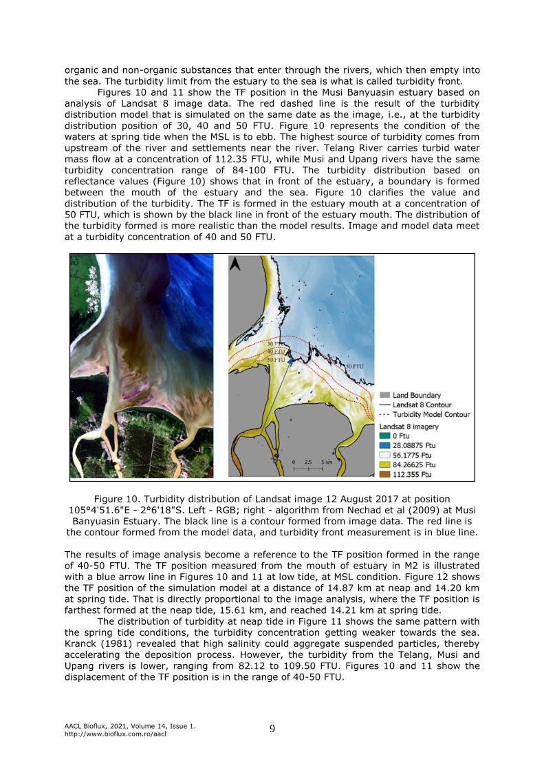
organic and non-organic substances that enter through the rivers, which then empty into

the sea. The turbidity limit from the estuary to the sea is what is called turbidity front.

Figures 10 and 11 show the TF position in the Musi Banyuasin estuary based on

analysis of Landsat 8 image data. The red dashed line is the result of the turbidity

distribution model that is simulated on the same date as the image, i.e., at the turbidity

distribution position of 30, 40 and 50 FTU. Figure 10 represents the condition of the

waters at spring tide when the MSL is to ebb. The highest source of turbidity comes from

upstream of the river and settlements near the river. Telang River carries turbid water

mass flow at a concentration of 112.35 FTU, while Musi and Upang rivers have the same

turbidity concentration range of 84-100 FTU. The turbidity distribution based on

reflectance values (Figure 10) shows that in front of the estuary, a boundary is formed

between the mouth of the estuary and the sea. Figure 10 clarifies the value and

distribution of the turbidity. The TF is formed in the estuary mouth at a concentration of

50 FTU, which is shown by the black line in front of the estuary mouth. The distribution of

the turbidity formed is more realistic than the model results. Image and model data meet

at a turbidity concentration of 40 and 50 FTU.

Figure 10. Turbidity distribution of Landsat image 12 August 2017 at position

105°4'51.6"E - 2°6'18"S. Left - RGB; right - algorithm from Nechad et al (2009) at Musi

Banyuasin Estuary. The black line is a contour formed from image data. The red line is

the contour formed from the model data, and turbidity front measurement is in blue line.

The results of image analysis become a reference to the TF position formed in the range

of 40-50 FTU. The TF position measured from the mouth of estuary in M2 is illustrated

with a blue arrow line in Figures 10 and 11 at low tide, at MSL condition. Figure 12 shows

the TF position of the simulation model at a distance of 14.87 km at neap and 14.20 km

at spring tide. That is directly proportional to the image analysis, where the TF position is

farthest formed at the neap tide, 15.61 km, and reached 14.21 km at spring tide.

The distribution of turbidity at neap tide in Figure 11 shows the same pattern with

the spring tide conditions, the turbidity concentration getting weaker towards the sea.

Kranck (1981) revealed that high salinity could aggregate suspended particles, thereby

accelerating the deposition process. However, the turbidity from the Telang, Musi and

Upang rivers is lower, ranging from 82.12 to 109.50 FTU. Figures 10 and 11 show the

displacement of the TF position is in the range of 40-50 FTU.



Figure 11. Turbidity distribution of Landsat image 20 July 2018 at position 105°4'51.6"E -

2°6'18"S. Left - RGB; right - algorithm after Nechad et al (2009) at Musi Banyuasin

Estuary. The black line is a contour formed from image data. The red line is the contour

formed from the model data and TF measurement is shown by the blue line.

Figure 12. Distribution of turbidity model and Landsat 8 imagery low tide to mean sea

level.

The distribution of turbidity at neap tide is farther from the spring tide. However, the

turbidity concentration at spring tide is higher than at neap tide. Strong tidal forces at

spring tide stir the bottom sediment, which is lifted to the surface, so that the turbidity

concentration increases and is distributed vertically (Mashyur et al 2018). At neap

conditions, the mass of water is smaller than average. Meaning that high tides are

somewhat lower and low tides are somewhat higher. In this condition, freshwater flows

to estuary, while the seawater is pulled out, which also brings turbidity flow spreads

further to the sea and cause TF to form even farther.

The turbidity distribution correlation of satellite images and models (Figure 13)

shows the same pattern with the correlation coefficient r=0.64 for image acquisition on

August 12, 2018, and r=0.67 for an image on August 18, 2018. The correlation between

turbidity of the image and model, 0.5<r<0.7, shows a strong relationship (Suprapto

2001).



Figure 13. Correlation of Landsat Image 8 data and models on acquisition (a) on July 20,

2017, and (b) on August 12, 2018.

Tidal excursion. Tidal excursion describes the distance distribution of particles in the

mouth of the estuary based on the tidal cycle (Savenije 2012). The amplitude velocity

component (vo) K1, as the dominant component in the MBE, was used to calculate the

tidal excursion. The tidal excursion distance is 4.8 km from M2 (Figure 1) to the sea or

10.8 km from the measurement points in Figures 10 and 11. The tidal excursion distance

and the maximum TF position at the time of the tide have a difference of 4.07 km.

The difference is due to the massive debit flow from the Musi River (202.15 m3

s-1) and Telang River (142.6 m3 s-1). The massive debit flow restrains the current in the

estuary’s mouth in high and low conditions, and cause the current velocity at the M2

location to be low, so that the vo issued is also small, at 0.162 m s-1 for the K1

component. This is also influenced by the difference in time of collecting data, current

speed and image data.

Conclusions. The distribution of turbidity in the Musi Banyuasin estuary is strongly

influenced by the hydrodynamic processes, especially tides. The tidal cycle, with neap

and spring tide, is a factor that determines the position of the turbidity front. The TF from

image analysis that has been confirmed by the turbidity distribution model is formed in

the turbidity range of 40-50 FTU. The TF position, from the model simulation results and

image analysis, shows that the farthest distance formed at the peak is 14.87 km in the



model data and 15.61 km in the image data. In the spring tide conditions, the distance of

the TF position is 14.20 km for the model data and 14.21 km for image data. The

difference in TF distance in both data, for neap and spring tide, is less than 1.18 km.

Acknowledgements. Special thanks to Denny Alberto Satrya Gumay and Lerma Yuni

Siagian for providing field data. Thank also go to those who helped provide input and

suggestions in writing.

References

Blaber S. J. M., 1997 Fish and fisheries in tropical estuaries. Springer Netherlands, 367 p.

Derisio C., Braverman M., Gaitan E., Hosbor C., Ramirez F., Carreto J., Botto F.,

Gagliardini D. A., Acha E. M., Mianzan H., 2014 The turbidity front as a habitat for

Acartia tonsa (Copepoda) in the Río de la Plata, Argentina-Uruguay. Journal of Sea

Research 85:197-204.

Dogliotti A. I., K. Ruddick K. G., Nechad B., Doxaran D., Knaeps E., 2015 A single

algorithm to retrieve turbidity from remotely-sensed data in all coastal and

estuarine waters. Remote Sensing of Environment 156:157-168.

Dogliotti A. I., Ruddick K., Nechad B., Lasta C., Mercado A., Hozbor C., Guerrero R.,

Lopez G. R., Abelando M., 2011 Calibration and validation of an algorithm for

remote sensing of turbidity over La Plata river estuary, Argentina. EARSeL

eProceedings 10:119-130.

Elliott M., McLusky D. S., 2002 The need for definitions in understanding estuaries.

Estuarine, Coastal and Shelf Science 55(6):815-827.

Ge J., Torres R., Chen C., Liu J., Xu Y., Bellerby R., Shen F., Bruggeman J., Ding P., 2020

Influence of suspended sediment front on nutrients and phytoplankton dynamics off

the Changjiang Estuary: A FVCOM-ERSEM coupled model experiment. Journal of

Marine Systems 204:103292, 19 p.

Kranck K., 1981 Particulate matter grain-size characteristics and flocculation in a partially

mixed estuary. Sedimentology 28(1):107-114.

Masyhur E. M. H., Jusoh W. N. W., Bakar M. N. A., 2018 Field study to identify river

plume extention of Kerian river discharge during neap and spring tide. Bulletin of

Geological Society of Malaysia 65:13-18.

Nechad B., Ruddick K. G., Neukermans G., 2009 Calibration and validation of a generic

multisensor algorithm for mapping of turbidity in coastal waters. SPIE Remote

Sensing, Proceedings Volume 7473, Remote sensing of the ocean, sea ice, and large

water regions, Berlin, 11 p.

Nechad B., Ruddick K. G., Park Y., 2010 Calibration and validation of a generic

multisensor algorithm for mapping of total suspended matter in turbid waters.

Remote Sensing of Environment 114(4):854-866.

Nurdjaman S., Burhanuddin M. N., Yanagi T., Radjwane I. M., Suprijo T., 2018 Estimating

flushing time in Citarum River Estuary, Indonesia by using empirical and numerical

methods. AES Bioflux 10(3):209-216.

Nurisman N., Surbakti H., Fauziah, 2012 [Tidal characteristics in the Musi River cruise

line using the admiralty method]. Maspari Journal 4(1):110-115. [In Indonesian].

Nurjaya I. W., Surbakti H., Natih N. M. N., 2019 Model of total suspended solid (TSS)

distribution due to coastal mining in western coast of Kundur Island part of Berhala

Strait. IOP Conference Series: Earth and Environmental Science 278:012056, 17 p.

Purwiyanto A. I. S., 2015 [Distribution and adsorption of lead metal (Pb) at Muara Sungai

Banyuasin, South Sumatra]. Indonesian Journal of Marine Sciences 20(3):153-162.

[In Indonesian].

Putri W. A. E., Bengen D. G., Prartono T., Riani E., 2016 [Accumulation of heavy metals

(Cu and Pb) in two consumed fishes from Musi River Estuary, South Sumatera].

Indonesian Journal of Marine Sciences 21(1):45-52. [In Indonesian].

Radjwane I. W., Saputro B. S. C., Egon A., 2018 [Tidal hydrodynamic model in Bangka

Belitung Islands]. Jurnal Teoritic dan Terapan Bidang rekayasa Sipil 26(2):121-128.

[In Indonesian].



Sari C. I., Surbakti H., Fauziah, 2013 [Salinity distribution pattern with a two-dimensional

numerical model at the mouth of the Musi River]. Maspari Journal 5(2):104-110. [In

Indonesian].

Savenije H. H. G., 2012 Salinity and tides in alluvial estuaries. Gulf Professional

Publishing, 194 p.

Schacht C. M., Lemckert C. J., 2003 Quantifying the estuarine surface-sediment

dynamics in the Brisbane River. Coasts and Ports Australian Conference:

Proceedings of the 16th Australasian Coastal and Ocean Engineering Conference, the

9th Australasian Port and Harbour Conference and the Annual New Zealand Coastal

Society Conference, 31 p.

Simatupang C. M., Surbakti H., Agussalim A., 2016 [Analysis of the flow data in the

mouth of the Banyuasin River in the southern Sumatra province]. Maspari Journal

8(1):15-24. [In Indonesian].

Sinaga H., Surbakti H., Diansyah G., 2019 [Mangrove zoning and its relation to salinity in

the Sungai Upang estuary, Banyuasin district, southern Sumatra]. Jurnal Penelitian

Sains 21(2):66-77. [In Indonesian].

Suprapto J., 2001 [Statistics theory and applications]. Erlangga, Jakarta, 370 p. [In

Indonesian].

Surbakti H., 2012 [The characteristics of the ebb and flow pattern in Musi River estuary,

southern Sumatra]. Jurnal Penelitian Sains 15:35-39. [In Indonesian].

Surbakti H., Isnaini, Aryawati R., 2014 [Water mass characteristics in the estuaries of the

Banyuasin River]. Prosiding Seminar Nasional MIPA, Palembang: FMIPA Universitas

Sriwijaya, pp. 511-515 p. [In Indonesian].

Suteja Y., Purwiyanto A. I. S., Agustriani F., 2019 [Mercury (Hg) on the surface of the

mouth of the Banyuasin River, South Sumatra, Indonesia]. Journal of Marine and

Aquatic Sciences 5(2):177-184. [In Indonesian].

Yu Y., Zhang H., Lemckert C., 2014 Salinity and turbidity distributions in the Brisbane

River estuary, Australia. Journal of Hydrology 519:3338-3352.

Zaman B., Syafrudin, 2007 [2-D numerical model (lateral & longitudinal) distribution of

cadmium (Cd) pollutants in river estuaries (case study: Babon River estuary,

Semarang]. Jurnal Presipitasi 3(2), 8 p. [In Indonesian].

Zhen-Gang J., 2008 Hydrodynamics and water quality: Modeling rivers, lakes and

estuaries. John Wiley and Sons, pp. 576-580.

***BPS (Central Statistics Agency) of South Sumatra Province, 2016 [South Sumatra

Province in figures 2016]. Palembang, Indonesia. [In Indonesian].

***https://earthexplorer.usgs.gov/

Received: 25 June 2020. Accepted: 26 August 2020. Published online: 01 January 2021. Authors: Septy Heltria, IPB University, Faculty of Fisheries and Marine Science, Department of Marine Science and Technology, 16680 Bogor, Indonesia, e-mail: [email protected] I Wayan Nurjaya, IPB University, Faculty of Fisheries and Marine Science, Department of Marine Science and Technology, 16680 Bogor, Indonesia, e-mail: [email protected] Jonson Lumban Gaol, IPB University, Faculty of Fisheries and Marine Science, Department of Marine Science and Technology, 16680 Bogor, Indonesia, e-mail: [email protected] This is an open-access article distributed under the terms of the Creative Commons Attribution License, which permits unrestricted use, distribution and reproduction in any medium, provided the original author and source are credited. How to cite this article: Heltria S., Nurjaya W. I, Gaol J. L., 2021 Turbidity front dynamics of the Musi Banyuasin Estuary using numerical model and Landsat 8 satellite. AACL Bioflux 14(1):1-13.

Documents

Turbidity front dynamics of the Musi Banyuasin Estuary