Embed Size (px)
Citation preview

UNIVERSITA DEGLI STUDI DI PADOVADIPARTIMENTO DI ELETTRONICA ED INFORMATICA
DOTTORATO DI RICERCA IN INGEGNERIA INFORMATICA EDELETTRONICA INDUSTRIALI
XIII CICLO
VISIONI DI UNA TEORIA DELLEPROBABILITA GENERALIZZATE
Coordinatore: Ch.mo Prof. Massimo Maresca
Supervisore: Ch.mo Prof. Ruggero Frezza
Dottorando: Fabio Cuzzolin
31 gennaio 2001

Abstract
Computer vision is an increasingly growing discipline with the ambitious purpose of en-abling machines to mimic the visual skills humans and animals are provided by the na-ture, allowing them to move effortless inside complex, dynamic environments. Designingautomatic recognition and sensing systems involves a number of very difficult tasks andrequires a large variety of interesting and even sophisticated mathematical tools. In mostcases the knowledge the animal or automatic agent has of the external world is at leastuncompleted or even missing at all. The need of a mathematical description of uncertainmodels and measurements naturally arises.The theory of evidence is perhaps one of the most successful approaches to uncertaintytheory and surely the most straightforward and intuitive attempt to produce a generalizedprobability theory. Coming out from a deep criticism of the classical Bayesian theory ofinference, it stimulated a wide discussion about the epistemic nature of beliefs and chances.During the last decade, a renewed interest in generalized probabilities or belief functionshas seen the born of many applications of this theory, mainly in the field of sensor fusion.
In this thesis we are going to show how the mutual interaction of vision and evidentialreasoning can produce a number of new interesting results on both sides. We will de-scribe some theoretical advances about the geometrical and algebraic properties of belieffunctions, and introduce in the theory a well-known concept of probability theory such asthat of total function. The introduction of tools widely used in computer and system en-gineering is definitively necessary to achieve the goal of a valid alternative to the classicalBayesian formalism.On the other side we will explain how these questions arise from classical computer visionproblems, namely articulated object tracking, data association and feature integration. Allthese problems will find a natural solution in the framework of the evidential reasoning andstimulate the comparison between evidential and probabilistic approaches.
3

Sommario
La visione computazionale e una disciplina in crescente sviluppo, avente l’ambizioso com-pito di dotare le macchine di quelle capacita visive di cui uomini e animali sono dotatidalla natura, e che permettono loro di interagire senza difficolta in ambienti mutevoli ecomplessi. La progettazione di sistemi di visione e riconoscimento automatico comportauna quantita di difficili problemi, che richiedono per essere risolti una grande varieta diinteressanti e talvolta sofisticati strumenti matematici. Nella maggior parte dei casi laconoscenza che l’animale o l’agente artificiale ha del mondo esterno e quantomeno in-completa, o addirittura del tutto mancante. Emerge cosı naturalmente il bisogno di unadescrizione matematica di modelli e misure affetti da incertezza.La teoria dell’evidenza (dall’inglese theory of evidence) e forse uno dei piu fortunatiapprocci nel campo della descrizione dell’incertezza, e sicuramente il tentativo piu di-retto e intuitivo di produrre una teoria delle probabilita generalizzate. Nata da profondecritiche alla teoria classica di inferenza Bayesiana, ha stimolato un’ampia discussionesulla natura filosofica delle probabilita, nella loro doppia interpretazione in termini di de-scrizione dell’evidenza in favore in una proposizione ovvero di frequenze relative di unevento associato ad un esperimento aleatorio. Durante il decennio scorso un rinnovatointeresse nelle probabilita generalizzate o belief function ha dato luogo a numerose appli-cazioni in campo ingegneristico, principalmente nell’ambito della cosiddetta sensor fusion.Lo scopo di questa tesi e quello di mostrare come l’interazione tra la visione e la teoriadell’evidenza possa produrre numerosi interessanti risultati in entrambi i campi. Da unlato, essa descrive alcuni risultati teorici riguardanti le proprieta algebriche e geometrichedelle belief function e introduce in questa disciplina l’analogo di un concetto ben noto inteoria della probabilita, quello di probabilita totale. Uno strumento, questo, largamenteusato in ingegneria informatica e dei sistemi, e la cui introduzione, insieme agli analoghidell’idea di processo aleatorio e di filtraggio, e necessaria per fare di questa teoria una val-ida alternativa al formalismo classico Bayesiano.Dall’altro mostreremo come queste questioni emergano da classici problemi di visione,quali l’inseguimento di un corpo articolato, la corrispondenza tra punti in immagini con-secutive e l’integrazione di misure estratte dall’immagine (features). Tutti questi problemitrovano una soluzione naturale nell’ambito della teoria dell’evidenza, stimolando nel con-tempo un confronto con l’approccio probabilistico.
5

”La vera logica di questo mondo e il calcolo delle probabilita ... Questa branca dellamatematica, che di solito viene ritenuta favorire il gioco d’azzardo, quello dei dadi e dellescommesse, e quindi estremamente immorale, e la sola ”matematica per uomini pratici”,quali noi dovremmo essere. Ebbene, come la conoscenza umana deriva dai sensi in modotale che l’esistenza delle cose esterne e inferita solo dall’armoniosa (ma non uguale) testi-monianza dei diversi sensi, la comprensione, che agisce per mezzo delle leggi del correttoragionamento, assegnera a diverse verita (o fatti, o testimonianze, o comunque li si vogliachiamare) diversi gradi di probabilita.”
James Clerk Maxwell

Contents
Abstract 3
Sommario 5
Chapter 1. Introduction 11
Part 1. Evidential reasoning 15
Chapter 2. Shafer’s mathematical theory of evidence 171. Belief functions 172. Dempster’s rule of combination 203. Simple and separable support functions 224. Families of compatible frames of discernment 245. Support functions 276. Impact of the evidence 287. Quasi support functions 298. Consonant belief functions 31
Chapter 3. Evidential reasoning’s state of the art 331. The origins: Dempster’s upper and lower probabilities 332. Philosophical discussion 353. Frameworks and approaches 364. Dempster’ rule of computation, propagation networks and algorithms 375. Theoretical advances 376. Statistical inference and estimation 397. Decision and classification 398. Generalizations and continuous formulations 409. Relations with other theories 4110. Applications 43
Part 2. Theoretical advances 47
Chapter 4. Geometric analysis of the belief space and conditional subspaces 491. Motivations 492. Belief space 503. Bundle structure 524. Simplicial form of the belief space 585. Commutativity 606. Conditional subspaces 617. Geometric interpretation of Dempster’s rule 638. Order relations 66
7

8 CONTENTS
9. Probabilistic approximations 6910. Comments 73
Chapter 5. Algebraic structure of the families of compatible frames 751. Motivations: measurement conflict 752. Axiom analysis 763. Monoidal structure 784. Lattice structure 825. Semimodularity 856. Comments 86
Chapter 6. Independence and conflict 871. Subspace and frame lattices 872. Frame lattice and external independence 883. Equivalence of internal and external independence 984. Conflicting evidence and pseudo Gram-Schmidt algorithm 98
Chapter 7. Conditional belief functions and total belief theorem 991. Introduction 992. The data association problem 1003. Combining conditional functions 1044. The total belief theorem 1055. Solution systems and transformable columns 1076. Solution graphs 1097. Future work 111
Part 3. Computer vision applications 113
Chapter 8. Articulated object tracking 1151. Evidential model 1152. Conflict analysis 1243. Pointwise estimation 1264. Algorithms 1265. Experiments 1276. Comments 130
Chapter 9. Towards unsupervised action recognition 1331. Action recognition in unsupervised context 1332. Representation of actions 1353. Detecting actions in clutter 1364. Experiments 1385. The role of the evidential reasoning 141
Part 4. Conclusions and appendices 145
Chapter 10. Conclusions 147
Appendix A. Algebraic structures 1511. Posets and lattices 1512. Boolean algebras 154

CONTENTS 9
Bibliography 157

CHAPTER 1
Introduction
In the river of scientific research several streams interlaces often originating a richproduction of new results. The interaction between mathematics and physics, for example,marks out the foundation of modern science since the publication of Newton’s ”PhilosophiaNaturalis Principia Mathematica”
�
. The dramatic development of human knowledge dur-ing the last century has increased, on the one hand, the possibility of such fruitful relations:on the other this same growth has produced an apparently unavoidable trend to specializa-tion.The main goal of this thesis is to expose a complex example of fruitful contact betweenvery different disciplines.Computer vision is an increasingly growing discipline with the ambitious purpose of enablemachines to reproduce in same manner the visual skills humans and animals are providedby the Nature, allowing them to interact effortless with complex, dynamic environments.Designing automatic recognition and sensing systems involves a number of very difficulttasks requiring a wide variety of interesting and even sophisticated mathematical tools. Inmost cases the knowledge the animal or automatic agent has of the external world is at leastuncompleted or even missing at all. The need of a mathematical description of uncertainmodels and measurements naturally arises.In particular that is true when, at the beginning of its operative life, an agent must buildits own model of the external world from the sheer data it receives from its sensors. Thedata is often inherently imprecise, and has to be combined in order to increase the agent’sknowledge.
In the field of uncertainty description, the theory of evidence is perhaps one of the mostsuccessful approaches and surely the most straightforward and intuitive attempt to producea generalized probability theory. Coming out in the late Sixties from a deep criticism of theclassical Bayesian theory of inference, it stimulated a wide discussion about the epistemicnature of beliefs (i.e. one’s degrees of belief in a certain proposition or claim) and chances(i.e. the limit values of relative frequencies in random experiments).The basis notion is that of belief function, as mathematical description of the total beliefon propositions belonging to a set of possible answers, or frame of discernment, inducedby the evidence available at the moment. Shafer has tried to formalize the concept ofevidence supporting a proposition with quantitative strength, even if with some troubles.Belief functions carried by different bodies of evidence can be combined using the socalled Dempster’s rule: the combination rule is the attractive tool that permits the processof integrating information in order to make decisions or estimations.The theory has born as an application of standard probability theory (see Dempster’s paperson upper and lower probabilities, [97] and [99]): Dempster’s rule itself is a consequenceof the assumption of independence of some underlying probability. Nevertheless it hasbeen reorganized on an axiomatic basis by Glenn Shafer with its 1976’s essay ([410]).
�
Isaac Newton, 1687
11
12 1. INTRODUCTION
This two interpretations, belief functions as generalized probabilities, and belief functionsas independent description of partial beliefs, together with several others still continue toconvive at the present day.
Why a theory of evidence? In my own experience the most popular objection againstthe use of uncertainty management techniques alternative to standard probabilistic meth-ods is: why spending energy and efforts on learning a new more complicated theory onlyto satisfy philosophical curiosity? The implicit remark here is that probability is sufficientto solve any practical question arising in real-life problems. In most cases people agreewhen you point out the greater naturalness of evidential solutions to several questions butseem to regard it a matter of esthetic taste when well-established probabilistic techniquesexist.Belief functions are the most straightforward and natural way of extending classical prob-abilities, therefore they have the biggest chance of being accepted by the largest spectrumof scientist and researchers.In this thesis we will neglect almost completely the interpretation of belief functions interms of evidence, preferring their nature of generalized probabilities. In any case, we willnot bother the reader with vacuous debates about the existence of the correct approach touncertainty theory: our work on the theory of belief functions is strictly technical, andaimed to solve beautiful mathematical problems arising from equally interesting computervision questions. It suffices to point out that several authors (see Chapter 3) have supportedthe idea that a battery of tools has to be used according to the specific problem we have toface, without prejudices.
Objectives. During the last decade, a renewed interest in the evidential reasoning,and uncertainty description in general, has born mainly in the field of sensor fusion appli-cations, since the idea of combination of evidence is intuitively appealing in this context.A situation in which data coming from different cameras, or very different measurementsor features extracted by an image must be integrated in order to estimate, for example,the structure of a scene, or to decide what kind of action is being executed in front of thecamera is very common in vision.
We will describe a set of theoretical advances about the geometrical and algebraicproperties of belief functions and introduce in the theory a concept well-known in proba-bility theory such as that of total function. Our long-term goal is to introduce in the theorytools analogous to filtering and random processes, widely used in computer and systemengineering and definitively necessary to achieve the goal of a valid alternative to the clas-sical Bayesian formalism. The theory of evidence is relatively young, and still lacks anumber of tools, as we will point out. Its major limitation is of course that is bounded tofinite frames, even if a few attempts have been made to generalize it to continuous domains(for instance the theory of random sets).In this work we wish to make a first step in the direction of the completion of this math-ematical framework, whose complexity on the other sides generates problems completelynew for someone with a standard probabilistic background.
On the other side we will explain how these theoretical questions arise from classicalcomputer vision problems, namely articulated object tracking, data association, featureintegration and action recognition. All these problems can find a natural solution in theframework of the evidential reasoning and stimulate the comparison between evidentialand probabilistic approaches.
1. INTRODUCTION 13
Outline. The thesis is divided into three parts. In the first one we will introduce thecore of the evidential reasoning formalism (Chapter 2) along with the basis notions nec-essary to the comprehension of what follows, even if the limited space has prevented usto adopt a more didactic approach, for example by placing a large number of examples tohighlight the most important notions.As we mentioned above, many theories have been formulated in order to integrate or sub-stitute the classical theory for different reasons, ranging from philosophical to strictly ap-plicative ones. Some of these methods for the treatment of uncertainty are depicted inChapter 3, where we will attempt to give a comprehensive view of the matter, as it hasevolved during the last twenty years. A large sample of the recent theoretical advances to-gether with flavors of the applications present in the literature is given, included a sectionon computer vision tasks.
Part II is in a sense the core of the thesis. Starting from Shafer’s axiomatic formulationof the theory of belief functions, and motivated by the problems exposed in Part III, wewill introduce some new theoretical advances about the geometric and algebraic structureof belief functions themselves, and their domains.In Chapter 4 the geometric properties of belief functions are investigated, by reconstructingthe shape of the space of all the belief functions defined over a given domain (belief space).This will lead to a geometric description of the effect of conditioning and a geometricinterpretation of Dempster’s rule.In perspective, this geometric approach seems to be useful to solve important problems, forinstance the question of reconstructing the canonical decomposition of a belief functionin term of its simple components (see Chapter 2). The problem of finding the “right”probabilistic approximation of a b.f., necessary to extract pointwise estimates from a belieffunctions, can also find a natural formulation in this environment.Stimulated by the conflict problem, i.e. the fact that not every collection of belief function(representing for example image features) is combinable, in Chapter 5 we will analyze thealgebraic structure of the families of compatible frames of discernment (the finite domainsof belief functions), proving their lattice properties. In the next Chapter we will deepenthe notion of independence of frames, as elements of a semimodular lattice, and propose asolution to the conflict problem based on a pseudo-Gram-Schmidt algorithm.In (Chapter 7) we will discuss an evidential solution to the model-based data associationproblem, in which feature points measuring the positions of markers on a moving articu-lated body (for instance a human one) are detected at each time instant. Correspondencesbetween point in
�����and��������
must be found in presence of occlusions and miss-ing data, mainly by means of a battery of Kalman filters taking care of each point. Belieffunctions can be useful to integrate the logical information carried by a topological modelof the body with filter outcomes.In this context the necessity of combining combining conditional belief functions under aprior arises, leading to the evidential analogous of the total probability theorem. This is thefirst step, in our opinion, to a theory of filtering in the context of generalized probabilities.Unfortunately, only a partial solution to this total belief problem is given, together withhints of the future directions of the investigation.
In Part III we will illustrate the computer vision applications that have stimulated thesearch for new methods in the ToE.Chapter 8 expose the use of the evidential fusion scheme to solve the problem of estimatingthe pose and configuration of an articulated object with a number of degrees of freedom.In this context the question of conflicting measurements arises, together with the need to

14 1. INTRODUCTION
compute the probabilistic approximation of a belief estimate in order to get a pointwiseestimate of the object parameters.Chapter 9 introduce a long-term project on action recognition in an unsupervised context,i.e. when no a-priori knowledge about the nature of the motion is available. A first resulton the compositional property of the chosen model is shown, and the evidential reasoningis proposed for the final stage of the classification process.
Finally, a brief Appendix provides the indispensable basis for the algebraic analysis ofthe collections of frames and the idea of independence as developed in Chapters 5 and 6.
Part 1
Evidential reasoning

CHAPTER 2
Shafer’s mathematical theory of evidence
The theory of evidence[410] has been introduced in the late Seventies by Glenn Shaferas a way of representing epistemic knowledge, starting from a sequence of seminal works([93], [99], [100]) of Arthur Dempster, Shafer’s advisor. In this formalism the best repre-sentation of chance is a belief function (b.f.) rather than a Bayesian mass distribution. Theyassign probability values to sets of possibilities rather than single events: their appeal restson the fact they naturally encode evidence in favor to propositions. The theory embracesthe familiar idea of assigning numbers between 0 and 1 to indicate this degrees of supportbut, instead of focusing on how this numbers are determined, it concerns the combinationof degrees of belief.
The formalism provides a simple method for combining the evidence carried by anumber of different sources (Dempster’s rule) with no need of any a-priori distributions.In this sense, following Shafer, it can be seen as a theory of probable reasoning. A formaldefinition of the different levels of detail in knowledge representation is introduced, whenthe concept of family of compatible frames reflects the intuitive idea of different descrip-tions (features) of a same phenomenon.
The most popular theory of probable reasoning is perhaps the Bayesian theory, dueto the English clergyman Thomas Bayes (1702-1761), claiming that all degrees of beliefsmust obey the rule of chances (i.e. the proportion of the time one of the possible outcomesof a random experiment tends to occur, see Definition 1). Furthermore, the fourth rule ofthe Bayesian theory gives a precise way a Bayesian function must be updated when welearn that a certain proposition � is true:
������� �� ������� ����� �� �
it is called Bayes’ rule.We will see that the Bayesian theory is contained in the theory of evidence as a specialcase, since both Bayesian functions are belief functions, and Bayes’ rule is a special caseof Dempster’s rule of combination.
In the following we will neglect most of the emphasis Shafer puts on the notion ofweight of evidence, for we judged it unnecessary to the comprehension of what follows.
1. Belief functions
Let us first review the classical definition of probability measure, due to Kolmogorov.
DEFINITION 1. A probability measure over a � -field ������� associated to a samplespace � is a function ��������� � � �"! such that
# � �%$ � � � ;# � � �&� ��� ;# if � �� � $ �'�(� �*) � then � � �,+ � � � � � �� � � ��� � (additivity).
17
18 2. SHAFER’S MATHEMATICAL THEORY OF EVIDENCE
Now, if we relax the third constraint allowing the function to have the value obtainedby additivity as a lower bound, and restrict ourselves to finite sets, we obtain what Shafercalled a belief function.
DEFINITION 2. Suppose � is a finite set, and ��� denote the set of all subsets of � . Abelief function over � is a function � ����� � � � � �"! such that
# � �%$ � � � ;# � � � � ��� ;# for every positive integer � and every collection � � ��� � � � �� ) � �� � � � +� � � +��� ���� ���� � � � ���� ������� � � � �
�� � � � � � � � � � ��� � � � � �
� � � �� ���The third axiom, called superadditivity, obviously reduces to additivity when we substitutethe inequality with an equality: that is why belief functions can be seen as generalizationsof the familiar notion of finite probability.The domain � should be interpreted as a set of possible answers to a given problem, exactlyone of which is the correct one. For each subset (proposition) � ��� the quantity � � ��assumes the meaning of degree of belief that the truth lies in � .
Of course there would be no sense in claiming that these axioms are the exact math-ematical representation of degrees of belief: they can nevertheless be rigorously justified(see Chapter 3).
Example: the Ming vase. A simple example (extracted from [410]) can be useful fora first approach to these objects. We are looking to a vase that is represented as a productof the Ming dynasty, and wondering if it is genuine. If we call � � the possibility the vaseis original, and ��� the possibility it is counterfeit, then
� � � � � �!�"�"#is the set of possibility, and � $ ��� �!� � �!�"��#is the set of its subsets. A belief function � over � will represent the degree of beliefthat the vase is genuine as � �
� � � � � � # � , and the degree of belief the vase is a fake as�$� � � � � �"�"# � (note we refer to the subsets � � and �"� ). Axiom 3 of Definition 2 poses asimple constraint over � � and �$� : � �
� �$�&% � . The value of � in � , in a sense, representsevidence that cannot be committed to any precise answer.
1.1. Basic probability assignment. Following Shafer [410] we will call the finite setof possibilities frame
�
of discernment (FOD).
DEFINITION 3. A basic probability assignment (b.p.a.) over a FOD � is a function' ����� � � � � �"! such that ' �%$ � � � � (*) �' � �� ��� �
The quantity ' � �� is called basic probability number assigned to � and measure the beliefcommitted exactly to � ) ��� . The elements of ��� associated to non-zero values of m arecalled focal elements and their union core:+-, �� .(*) �*/ 01 (3254637
�8��
For a note about the intuitionistic origin of this denomination see Rosenthal, Quantales and their applica-tions[383].
1. BELIEF FUNCTIONS 19
Now suppose a b.p.a. is introduced over an arbitrary FOD.
DEFINITION 4. The belief function associated to the basic probability assignment mis defined as:
� � �� � � ) ( ' ��� �PROPOSITION 1. Definitions (2) and (4) are equivalent descriptions of the notion of
belief function.
Now we can understand the intuitive meaning of belief functions: � � �� represents the totalbelief committed to a set of possibilities � . As the above example teaches, belief functionsreadily lend themselves to the representation of ignorance, that is exactly the mass given tothe whole set of possibilities. The simplest belief function assigns all the basic probabilityto the whole frame � and is called vacuous belief function.The Bayesian theory, instead, finds some trouble with the representation of ignorance, forit cannot distinguish between lack of belief and disbelief: that is obviously due to theadditivity constraint,
��� �� � ������� ��� .The only way to represent absence of evidence is giving an equal degree of belief to everyoutcome in the frame: as we will see in Section 7.2 this produce incompatible results whenconsidering more refined descriptions of the same problem.
The basic probability assignment producing a given belief function can be uniquelyrecovered by means of the Moebius inversion formula �' � �� � � ) ( � � � �
� (�� � � � ��� ���(1)
so that there is a 1-1 correspondence between the set functions '�� � .1.2. Degree of doubt and upper probabilities. Other expressions of the evidence
producing a belief function � are the degree of doubt � � �� �� � ����� and, more important,the upper probability
� � �� ���� ��� � �� ��� � � �����(2)
that expresses the plausibility of a proposition � or, in other words, the amount of evidencenot against � . Again,
� convey the same information of � , and can be expressed as� � �� � � � ( 46�� '
��� ����� � ����1.3. Bayesian theory as a limiting case. As we have anticipated above, in the theory
of evidence a probability function is simply a peculiar belief function which satisfies theadditivity rule for disjoint sets.
DEFINITION 5. A Bayesian belief function is a belief function � satisfying the addi-tivity condition:
� � �� � � ���� � ��� �Obviously it meets the axioms of Definition 2 too, so that a Bayesian b.f. is a belief
function. It can be proved that
�See [505] for an explanation in term of the theory of monotone functions over partly ordered sets.
20 2. SHAFER’S MATHEMATICAL THEORY OF EVIDENCE
PROPOSITION 2. A function � is Bayesian ��� ��� � � � � � �"! such that
��� �� � ��� � � � � � �� � ��� ( � � ��� � � ���&�2. Dempster’s rule of combination
Belief functions representing distinct bodies of evidence are combined together by meansof Dempster’s rule of combination, or orthogonal sum.
DEFINITION 6. The orthogonal sum � ��� �$� of two belief functions is a function whosefocal elements are all the possible intersections between the combining focal elements andwhose b.p.a. is given by
' � �� � �
� / (� � � � 6 (
' �� ��� ' � ��� � �
� � �� / (� � � � 6��
' �� ��� ' � ��� � � �(3)
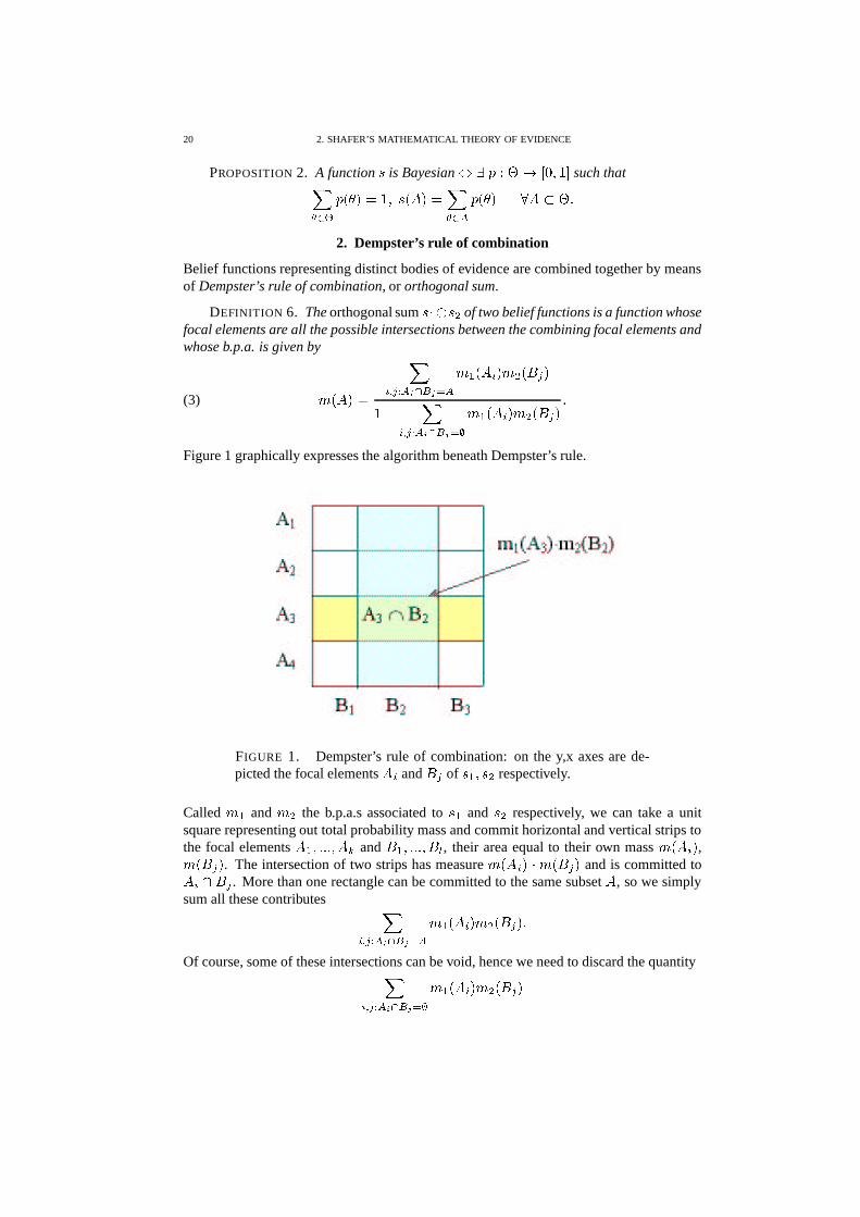
Figure 1 graphically expresses the algorithm beneath Dempster’s rule.
FIGURE 1. Dempster’s rule of combination: on the y,x axes are de-picted the focal elements �
�and
� �of � � � �$� respectively.
Called ' � and ' � the b.p.a.s associated to � � and �$� respectively, we can take a unitsquare representing out total probability mass and commit horizontal and vertical strips tothe focal elements � � ��� � � � ��� and
�� ��� � � � ��� , their area equal to their own mass ' � � � � ,' ��� � � . The intersection of two strips has measure ' � � � ��� ' ��� � � and is committed to
�� �� �
. More than one rectangle can be committed to the same subset � , so we simplysum all these contributes
�� / (� � � � 6 (
' �� ��� ' � ��� � ���
Of course, some of these intersections can be void, hence we need to discard the quantity
�� / (� � � � 6��
' �� ��� ' � ��� � �
2. DEMPSTER’S RULE OF COMBINATION 21
by normalizing the resulting basic probability assignment.It is important to note that two belief functions are combinable iff their cores are disjoint.
PROPOSITION 3. If � � � �$� are belief functions over the same frame � , then the fol-lowing conditions are equivalent:
# � � � �$� does not exists;# their cores are disjoint,+ , � +-, � � $
;# � � � � s.t. � �� �� � �$� ����� � � .
2.1. Combinability. The normalization constant in the above expression measuresthe level of conflict between belief functions for it represents the amount of probabilitythey attribute to contradictory (i.e. disjoint) subsets.
DEFINITION 7. We call level of conflict between�����
� and����� � the logarithm of the
normalizing constant in the Dempster’s rule� � ��� �
� � � � � / (� � � � 6�� ' �� ��� ' � ��� � �
It is interesting to note that weights of conflict combine additively:
PROPOSITION 4. Suppose � � ��� � � � �$��� � are belief functions over a frame � , and sup-pose � � � � � � � �$��� � exists. Then� � � � ��� � � � �$��� � � � � � � � ��� � � � �$� � � � � � � � � � � � �$� � �$��� � ���These concepts are easily extended to the general case of combining several belief func-tions, by simply iterating the algorithms explained above.
2.2. Conditioning belief functions. Dempster’s rule describes the way the assimila-tion of new evidence ��� changes our beliefs previously encoded into a function � , determin-ing new beliefs given by � � ��� � �� . This way a new body of evidence is not constrained tobe in the form of a single proposition known with certainty, still essential to the Bayesiantheory. Yet the assimilation of new certainties is permitted as a special case.In fact, this kind of evidence is represented by belief functions of the form
� � � �� ��� � ����� � � �
� ��� ���� �where
�is the certain proposition. Such a b.f. is combinable with � as long as � ���� ��� � ,
and the result has the form
� � � � � � �� � � � � � � �� �,+ �� ��� � �
� �� �� � � �
� �� �or, using the upper probabilities,
� �� � � � � �
� �� � �� ��
���� �(4)
an expression that is very similar to the Bayes’s rule of conditioning and Shafer calls Demp-ster’s rule of conditioning.
22 2. SHAFER’S MATHEMATICAL THEORY OF EVIDENCE
2.3. Combination vs conditioning. The way the new evidence is combined with apreviously existing belief function, by means of Dempster’s rule, is clearly symmetrical(due to the commutativity of set-theoretical intersection).In the Bayesian theory, instead, we are constrained to represent the new evidence as aprobability, and condition the Bayesian prior on that proposition. There is no obvioussymmetry, but far more important we must assume the impact of that new evidence is tosupport a single proposition with certainty!
3. Simple and separable support functions
A body of evidence usually supports a number of propositions of a frame of discernment,but the simplest situation is that where the evidence points to a single non-empty subset� � � . If � % � % � is the degree of support for � , the degree of support for a generic� ��� is given by
� ��� � ������������� ��� ���� �
� ��� � � �(� � �� �� ��� � � �
(5)
DEFINITION 8. The function � � ��� � � � � �"! defined by Equation (5) is called asimple support function focused on � ; its b.p.a is ' � �� � � , ' � � � � � ��� and ' ��� � �� for every other
�.
3.1. Heterogeneous and conflicting evidence. We often need to combine evidencepointing to different subsets, � and
�, of our frame of discernment. When � � �� $
this two propositions are compatible, and we say the related belief functions representheterogeneous evidence. In this case, if � � and �-� are the masses committed to � and
�by two simple support functions � � and �$� respectively, we get' � � � � � � � �-��� ' � �� � � �
� � � �-� � � ' ��� � � �-� � � � � � � � ' � � � � � � � � � � � � � �-� �so that
� ��� � �
�����������������������������������
� � �� � �
� � �-� � � � � � � �� �(� �
� �� � �(� � �� �
�-� � � � � � �� �� � � � � � � � � � � �-� � � � �(� � � � �� �� � � �
This means that the combined evidence supports � �with degree � � �-� , as our intuition
would suggest.Instead, when � � � $
we say the evidence being conflicting: in this situation thetwo bodies of evidence reduce the effect of the other. For example, the introduction of ���reduces the degree of support for � from � � to
� � �� � �$�� � � � �$� �
3. SIMPLE AND SEPARABLE SUPPORT FUNCTIONS 23
Example: the alibi. A criminal defendant has an alibi: a close friend swears thatthe defendant was visiting his house during at the time of the crime. This friend has agood reputation: suppose this commits a degree of support of
��� � � to the innocence of thedefendant ( � ). On the other side, there is a strong, actual body of evidence providing adegree of support of � � � � for his guilt ( � ).Formalizing, � � � � ����# , the friend provides a simple support function focused on
� ��#with ��� � � ��# � � ��� � � , while the other evidence corresponds to another simple supportfunction ��� focused on
� � # with �� � � � # � � � � � � . The orthogonal sum yields
� � � ��# � � ��� � � � � � � � # � �� ��� � � �the effect of the testimony has mildly eroded the force of the circumstantial evidence.
3.2. Separable support functions and decomposition. In general, belief functionscan support more than one proposition at a time: the next simplest class of b.f. is that ofseparable support functions.
DEFINITION 9. A separable support function is a belief function that is simple, or isequal to the orthogonal sum of two or more simple support functions, namely
� � � � � � � � � �$�where � � � , � � simple � i.
A separable support function can be decomposed in different ways; for example, given oneof this decompositions � � � � � � � �$� with foci � � ��� � � � �� and
+the core of � , all of the
following# � � � � � � � � � �$� � �$��� � where �$��� � is the vacuous b.f.;
# � � � � � � �$� � � � � � � �$� , if � �� �� ;
# � � ��� � � � � � � ���� , where ���� is the simple support function focused on � �� �� �� +
with ���� � � �� � , if �� + �� $
for all�;
are valid decompositions in terms of simple belief functions.On the other side
PROPOSITION 5. If � is a non-vacuous separable support function with core+3,
thenthere exists a unique collection � � ��� � � � �$� of non-vacuous simple support functions satisfy-ing the following conditions:
1. � � � ;2. � � � � if � ��� , and � � � � � � � � � �$� if � � � ;3.+-, � +-, ;
4.+-, �� +-, � if
� �� �.
This unique decomposition is called canonical decomposition.An intuitive idea of what a separable support function is, is given by the following result.
PROPOSITION 6. If � is a separable belief function, � and�
two of its focal elements,and � � �� $
, then � �is a focal element of � .
In other words, � is coherent in the sense that if it supports two proposition, then it mustsupport the proposition naturally implied by them, i.e. their intersection. That gives us asimple method to check if a given b.f. is a separable support function.

24 2. SHAFER’S MATHEMATICAL THEORY OF EVIDENCE
3.3. Internal conflict. Since a separable support function can support pairs of disjointsubsets, it indicates the existence of internal conflict.
DEFINITION 10. The weight of internal conflict �,
for a separable support function� is# 0 if � is a simple support function;#�� ��� � � � � ��� � � � �$� � for the various possible decompositions into simple support func-
tions � � � � � � � � � �$� if � is not simple.
It is easy to see (see [410] again) that �, � � � � � ��� � � � �$� � where � ��� � � � � �$� is its
canonical decomposition.
4. Families of compatible frames of discernment
4.1. Refinings. One of the amazing ideas in the D-S theory is the simple claim thatour knowledge of a given problem is inherently imprecise. New amount of evidence couldallow us to take decisions over more refined environments.One frame is certainly compatible with another if it can be obtained by introducing newdistinctions, i.e. by analyzing or splitting some of its possibilities into fine ones. Thisargument is embodied into the notion of refining.
DEFINITION 11. Given two frames � and � , a map � � ����� � � is a refining if itsatisfies the following conditions:
1. � � � � # � �� $ � � ) � ;2. � � � � # � � � � � ��# � � $ ��� � �� � � ;3. + ��� � � � � � # � � � .
The finer frame is called a refinement of the first one and we call � a coarsening of � . Boththe frames represents sets of possible answers to a given decision problem (see Chapter 3,too) but the finer one is a more detailed description, obtained by splitting each possibleanswer � ) � . � � �� will consists of all the possibilities in � that are obtained by splittingthe elements of � .Let us see some of the properties of refinings.
PROPOSITION 7. Suppose � ��� � � � � is a refining. Then# � is 1-1;# � �%$ � � $
;# � � � � � � ;# � � � + � � � � � �� +�� ��� � ;# � ����� � � � �� ;# � � � �� � � � � �� � ��� � ;# if �(� � � � then � � �� ��� ��� � iff � � �;# if �(� � � � then � � �� � ��� � � $
iff � �� � $.
A refining � � ��� � � � is not, in general, onto; in other words, there are subsets� � �
that are not images of subsets � of � . Nevertheless, there two different ways of associatingeach subset of the refinement to a subset of the coarsening.
DEFINITION 12. The inner reduction associated to a refining � is the map � � � � ���� given by
� � �� � � � ) � � � � � � # � � � #
4. FAMILIES OF COMPATIBLE FRAMES OF DISCERNMENT 25
DEFINITION 13. The outer reduction associated to a refining � is the map���� � � �
��� given by�� � �� � � � ) � � � � � � # � � �� $ #
Roughly speaking, � � �� is the largest subset of � that implies A while�� � �� is the smallest
subset of � that is implied by A. In fact,
PROPOSITION 8. Suppose � � ���,� � � is a refining, � ��� and� � � . Let
�� and� the outer and inner reduction for � . Then � ��� � � � iff� � � � �� , and � � � ��� � iff�� � �
.
4.2. Families of frames. Provided this basis tools the intuitive idea of different de-scriptions of a same phenomenon is encoded by the concept of family of compatible frames(see [410], pages 121-125).
DEFINITION 14. A non-empty collection of finite non-empty sets�
is a family ofcompatible frames of discernment with refinings � , where � is a non-empty collection ofrefinings between couples of frames in
�, if�
and � satisfy the following requirements:
1. composition of refinings: if � � � ��� � ����� � and ��� � ��� � � ����� are in � , then� ��� ��� is in � ;
2. identity of coarsenings: if � � � ��� � � � � and ��� � ��� � � � � are in � and��� �
) � � � �"� ) � � ����� � � � � � �� � � � # � � ��� � � �"�"# � then � �
� � � and� �� ��� ;
3. identity of refinings: if � � ����� � � � and ��� ����� � � � are in � , then � �� ��� ;
4. existence of coarsenings: if � )��and � � ��� � � � �� is a disjoint partition of � then
there is a coarsening in�
corresponding to this partition;5. existence of refinings: if � ) � )��
and � )��then there exists a refining
� ����� � � � in � and � )��such that � � � � # � has n elements;
6. existence of common refinements: every pair of elements in�
has a commonrefinement in
�.
The basic idea, here, is that two frames are compatible iff they concern proposition relatedone to the other, i.e. can be expressed as proposition in a common, and finer, frame.From property (6) a collection of compatible frames has many common refinements. Oneof these is particularly simple.
THEOREM 1. If � � ��� � � ��� � are elements of a family�
then there exists a unique ele-ment � )��
such that
1. � � � � � ����� � � � refining;2. � � ) � � � � ) � � � ��� � ��� ��� � � �!� ����� � � � �� � # � � �
� � � � # � � � � ��� � � �"� # ���(6)
This unique FOD is called the minimal refinement � ��� � � � � � � of the collection� � ��� � � ��� � . It is the simplest space in which you can compare propositions belonging todifferent compatible frames. In fact,
PROPOSITION 9. If � is a common refinement of � � ��� � � ��� � , then � ��� � � � � � � is acoarsening of � . Furthermore, � ��� � � � � � � is the only common refinement of � � ��� � � ��� �that is coarsening of every other common refinement.
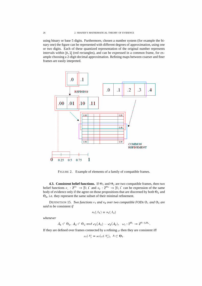
Example: number systems. Figure 2 illustrates a simple example of compatibleframes. A number between 0 and 1 can be expressed in several different basis, for instance
26 2. SHAFER’S MATHEMATICAL THEORY OF EVIDENCE
using binary or base 5 digits. Furthermore, chosen a number system (for example the bi-nary one) the figure can be represented with different degrees of approximation, using oneor two digits. Each of these quantized representation of the original number representsintervals within � � � �"! (red rectangles), and can be expressed in a common frame, for ex-ample choosing a 2-digit decimal approximation. Refining maps between coarser and finerframes are easily intepreted.
FIGURE 2. Example of elements of a family of compatible frames.
4.3. Consistent belief functions. If � � and � � are two compatible frames, then twobelief functions � � � ��� � � � � � �"! and �$��� ��� � � � � � �"! can be expression of the samebody of evidence only if the agree on those propositions that are discerned by both � � and� � , i.e. they represent the same subset of their minimal refinement.
DEFINITION 15. Two functions � � and �$� over two compatible FODs � � and � � aresaid to be consistent if
� �� � � � � �$� � �� �
whenever
� � ��� � �'�� ��� ������� � �� � � � � ��� � �� � � �
������ � ��� ��� � � �
If they are defined over frames connected by a refining � then they are consistent iff
� �� �� � �$� � � � �� � � � � � � �
5. SUPPORT FUNCTIONS 27
� � is called the restriction of � � to � � and you have' �� �� � ( 6��� 1 � 2
' � ��� ���(7)
4.4. Independent frames. Two compatible frames of discernment are independent ifno proposition discerned by one of them trivially implies a proposition discerned by theother. Obviously we need to refer to a common frame: for Proposition 9 it does not matterwhat common refinement we choose.
DEFINITION 16. Let � � ��� � � ��� � be compatible frames, and ��� ��� � ��� � ��� � � � � �
the corresponding refinings to their minimal refinement. They are said to be independent if
� �� � � � � � � ��� � �� � �� $
(8)
whenever$ �� �
�� � � for
� ��� ��� � � �!� .Equivalently, the above condition can be expressed as
# if ��� � � for
� � � ��� � � �!� and � �� � � � � � � ��� � �
� �� � � ��� ��� � �� � then�� � � � or one of the first � � � sets �
�is empty.
5. Support functions
Since Dempster’s rule of combination is applicable only to set functions satisfying theaxioms of belief functions (Definition 2), we are suggested to think that the class of belieffunctions is sufficiently large to describe the impact of a body of evidence on any frameof a family of compatible frames. Anyway, not all the belief functions are separable ones.Let us consider a body of evidence inducing a separable b.f. over a certain frame � of afamily
�: the impact of this evidence on a coarsening � of � is naturally described by the
restriction of � (Equation 7) to � .
DEFINITION 17. A belief function �(� ��� ��� � � �"! is a support function if there existssome refinement � of � and some separable support function � � � � ��� � � � �"! such that� � ��� � ��� .
As can be expected, not all the support functions are separable support functions. Thefollowing Proposition gives us a simple equivalent condition for this class of b.f.s.
PROPOSITION 10. Suppose � is a belief function, and+
its core. The following con-ditions are equivalent:
# � is a support function;# + has a positive basic probability number, ' � + � � � .
Since it is not necessary that ' � + � � � , Proposition 10 tells us that not all the belieffunctions are support ones.The impact of the evidence on a particular proposition � is adequately described by twovalues: the degree the evidence support � and its support to the negation
�� , or degree ofplausibility � � � �� ���� � � �����mathematically described by the upper probability (Equation (2))
�
. Hence, the plausibilityfunction
� �is another equivalent description of a support function, even if it is not in
general a belief function.�In its essay [410], Glenn Shafer distinguish between ”subjective” and ”evidential” vocabulary, keeping
distinct objects with the same mathematical description but different philosophical meaning.

28 2. SHAFER’S MATHEMATICAL THEORY OF EVIDENCE
5.1. Vacuous extension. There are occasions when the impact of a body of evidenceon a frame � is fully discerned by one of its coarsening � , i.e. no proposition discernedby � receive greater support than what is implied by propositions discerned by � .
DEFINITION 18. � � ��� � � � � �"! is the vacuous extension of � 7 � ��� � � � � �"! , where� is a coarsening of � , when
� � �� � ������ ) � �� 1 � 2 ) ( � 7��� � �
we say that � is carried by the coarsening � .
6. Impact of the evidence
6.1. Families of compatible support functions. We now know that a body of ev-idence
�simultaneously affects a whole family
�of compatible frames of discernment,
determining a support function over every element of�
. We say that�
determines a familyof compatible support functions
��� � # � �� . The complexity of this family depends on thefollowing property.
DEFINITION 19. The evidence�
affects�
sharply if there exists a frame � ) �that
carries� � for every � ) �
that is a refinement of � . Such a frame � is said to exhaustthe impact of
�on�
.
When � exhaust the impact of�
on�
,��� � # determines the whole family
��� � # � �� , forthe support function over any given frame � ) �
will be the restriction to � of��� � # ’s
vacuous extension to � � � . A typical example in which the evidence affects the familysharply is statistical evidence, where both frames and evidence are highly idealized. Onthe other side, it is difficult to put an a-priori limit on the specification of detail in theevidence.
6.2. Discerning the interaction of evidence. It is a commonplace that by selectingparticular inferences from a body of evidence and combining them with particular infer-ences from another body of evidence, one can derive almost arbitrary conclusions. In theevidential framework this remark is reflected by the fact that Dempster’s rule may produceinaccurate results when applied to inadequate frames of discernment. More precisely, letus consider a frame � , its coarsening � , and a pair of support functions � � � �$� on � deter-mined by two distinct bodies of evidence. By applying Dempster’s rule in � we obtain
� � � � �$� � � � � �while if we apply it in the coarser frame � the result is
� � �� � � � � � �$� � � � �
and in general will be different.
PROPOSITION 11. Suppose � � and �$� are support functions over a frame � ,�� ��� � �
��� an outer reduction, � � � �$� exists, and�� � � � � � �� � �� �� ��� �(9)
holds wherever � is a focal element of � � and�
is a focal element of � � . Then� � � � �$� � � � � � � � �
� � � � � � �$� � � � ���In this case � is said to discern the relevant interaction of � � and �$� . Of course if � � and�$� are carried by a coarsening then it discerns their relevant interaction.The above definition generalizes to entire bodies of evidence.
7. QUASI SUPPORT FUNCTIONS 29
DEFINITION 20. Suppose�
is a family of compatible frames,��� � � # � �� is the family
of support functions determined by a body of evidence�
� , and��� � � # � �� is the family of
support functions determined by the body of evidence� � . Then a particular frame � )��
is said to discern the relevant interaction of�
� and� � if
�� � � � � � �� � �� �� ��� �whenever � is a refinement of � ,
�� � � � � ��� is the outer reduction, � a focal element of� � � and�
a focal element of � �� .
7. Quasi support functions
Not every belief function is a support function, but we still do not know a precise de-scription of these “strange” objects. So, let us consider a finite power set � � : a sequence�
� � � � ��� � � of functions on ��� is said to tend to the limit�
if� � ������ � � � �� � � � �� � � ��� �it can be proved that
PROPOSITION 12. If a sequence of belief functions has a limit, then the limit is abelief function.
i.e. the class of belief functions is closed with respect to the convergence to a limit. Thisnew operation finally provides a solution to the nature of non-support functions.
PROPOSITION 13. If the belief function � is not a support function, then there existsa refinement � of � and a sequence � � � �$� ��� � � of separable support functions over � suchthat
� � � � � ������ � � � � � � �DEFINITION 21. We call these class quasi-support functions.
Remark. It can be noted that� � � ������ � � � � � � � � � ������ � � � � � � �
so we can also say that � is a limit of a sequence of support functions.
Let us try to understand the properties of quasi-support functions.
PROPOSITION 14. Suppose � is a belief function over � and � � � . If � � �� � � and� ����� � � , with � � �� � � ���� � ��� , then � is a quasi-support function.
It easily follows that most Bayesian b.f. are quasi-support functions. More precisely
PROPOSITION 15. A Bayesian belief function is a support function iff there exists � )� such that � � � � # � ��� .As Shafer remarks, people used to think to beliefs as chances can be disappointed
to see them relegated to a peripheral role, as beliefs that cannot arise from actual, finiteevidence. On the other side, statistical inference teaches us that chances can be evaluatedonly with infinite repetitions of independent random experiments. �
�Using its notion of weight of evidence Shafer gives a formal explanation of this intuitive observation by
showing that a Bayesian b.f. indicated an infinite amount of evidence in favor of each possibility in its core.
30 2. SHAFER’S MATHEMATICAL THEORY OF EVIDENCE
7.1. Bayes’ theorem. For it commits an infinite amount of evidence in favor of eachpossible answer, a Bayesian belief function obscures much of the evidence new belieffunctions carry with them.
DEFINITION 22. A function� � � � � � ���,� is said to express the relative plausibili-
ties of singletons under a support function � over � if� � ��� � � � � � � � # �for all � ) � , where
� �is the plausibility function for � and the constant does not depend
on � .PROPOSITION 16. (Bayes’ theorem) Suppose � 7 is a Bayesian belief function over� and � is a support function over � . Suppose
� ��� � � � ���,� expresses the relativeplausibilities of singletons under � . Suppose also � � � � � � 7 exists. Then ��� is Bayesian,and
� � � � � # � ��� �$� 7 � � � # � � � ��� � � ) �where
� � � ��� � �7 � � � # � � � ��� � � � �
That means that the combination of a Bayesian b.f. with a support function requires nothingmore than the relative plausibilities of singletons, not even
� � � �� for� � � � �
or theabsolute values. It is interesting to note that these functions behave multiplicatively undercombination.
PROPOSITION 17. If � � ��� � � � �$� are combinable support functions, and� �
representsthe relative plausibilities of singletons under � � for
� ��� ��� � � �!� , then�
� � � � � � � � � � � expressesthe relative plausibilities of singletons under � � � � � � � �$� .This way Proposition 16 may be used to combine any number of support functions with aBayesian function � 7 .
7.2. Incompatible priors. That could be useful if there was an established conven-tion about putting a Bayesian prior, avoiding us to make arbitrary choices that could affectthe final result. Unfortunately, the only natural convention to establish a Bayesian prior isstrongly dependent on the frame of discernment and is sensitive to refinement or coarsen-ing. More precisely, if we begin with a frame � with � elements, it is natural to adopt auniform priori as representation of our initial ignorance, assigning mass
��� � to every pos-sibility � ) � . The same convention applied to another compatible frame � of the familymay yield a prior that is incompatible with the first one: as a result, the combination ofevidence with one of these priors can yield almost any arbitrary result.
Example: Sirius’ planets. Some scientists ask themselves if there is life aroundSirius. Since they do not have evidence concerning this question, they adopt the vacuousbelief function as representation of their ignorance on the frame
� � � � � �!�"�"#where � � �!�"� are the answers “there is life” and “there is no life”. They can also considerthe question in the context of a more refined set of possibilities. For example, our scientistcan raise the question whether there even exist planets around Sirius. In this case the set ofpossibilities becomes
� � ��� � � � � � � � #
8. CONSONANT BELIEF FUNCTIONS 31
where�
� � � � � � � are respectively the possibility that there is life around Sirius, that thereare planets but no life, and there are no planets at all. Obviously our ignorance is stillrepresented by a vacuous b.f., that is exactly the vacuous extension of the previous one on� .From the Bayesian point of view, instead, it is difficult to pose consistent degrees of beliefover � and � symbolizing the lack of evidence. In fact, on � a uniform prior will yield� � � � � # � � � � � � � # � � ��� � , while on � the same choice will yield � � � ��� � # � � � � � ��� �"# � �� � � ��� � # � � ����� . But � and � are obviously compatible, and the extension of � onto �gives
� � ��� � # � � ����� � � � ��� � � � �"# � � � ���that is inconsistent with � � !
8. Consonant belief functions
At the opposite of quasi-support functions stand the so-called consonant belief functions.
DEFINITION 23. A belief function is said to be consonant if its focal elements arenested.
The following Proposition illustrates some of their properties.
PROPOSITION 18. If � is a belief function with upper probability function�
, thenthe following conditions are equivalent:
1. � is consonant;2. � � � �� � � � � � � � � �� � � ��� � � for every �(� � � � ;3.
� � �,+ � � � ����� ��� � �� � � ��� � � for every �(� � � � ;4.
� � �� � ����� ��� ( � � � � # � for all non-empty � � � ;5. there exists a positive integer � and simple support functions � � ��� � � � �$� such that� � � � � � � � � �$� and the focus of � � is contained in the focus of � � whenever
� � � .
Consonant b.f.s represents bodies of evidence pointing all towards the same direction;anyway, the evidence does not need to be completely nested, as the next Proposition states.
PROPOSITION 19. Suppose � � ��� � � � �$� are non-vacuous simple support functions withfoci+-, � ��� � � � +-, � respectively, and � � � � � � � � � �$� is consonant. If
+denotes the core of� , then the sets
+ , + are nested.
By condition 2 of Proposition 18 we have
� � � �%$ � � � � � ��� � ' � � � � � �� � � ���� � �i.e. either � � �� � � or � ����� � � for every ����� . This result and Proposition 14 explainwhy we said that consonant and quasi-support functions represent opposite sides of theclass of belief functions.


CHAPTER 3
Evidential reasoning’s state of the art
It the twenty years since its formulation the theory of evidence is obviously evolved,thanks to the work of several researchers, and now this denomination includes severaldifferent interpretations of the concept of generalized probability. A number of people haveproposed their own framework as the “correct” version of the evidential reasoning, partlyin response of deep critics sustained by important scientist of the field (see for instancePearl’s contribute in [356] and [357]). Several generalizations to continuous frames ofdiscernment have been attempt, even if none of them is still recognized as the definitiveanswer to the limitations of Shafer’s original formulation.In the last 10 years, the number of applications of the D-S theory to engineering and appliedsciences (mainly its fusion scheme based on the orthogonal sum) has started to increase,even if its diffusion is still limited compared to other more classical methods.A very good survey on the topic, from an original point of view, can be found in [256]; acomparative review about texts on evidence theory is presented in [372].
In this Chapter, we desire to give a flavor of the current state of development of thetheory of evidence, the various frameworks proposed during the years, the theoretical ad-vances achieved together with the algorithmic scheme (based mainly on propagation net-works) proposed to cope with the computational complexity of the rule of combination.The most popular evidential approaches to decision and inference are also reviewed, and abrief hint of the attempts of formulating a generalized theory valid for continuous sets ofpossibilities is given.Finally, the relation of Dempster-Shafer theory with other uncertainty theories and meth-ods is shortly depicted, and a sample of various applications to the most disparate fields isexposed, including a description of the few work has been done yet to propose evidentialsolutions to computer vision issues.
More references can be found in the bibliography, which is, with more 550 papers, thelargest collection of publications on the theory of evidence available at the moment.
1. The origins: Dempster’s upper and lower probabilities
The axiomatic set up that Shafer gave originally to his work could seem quite arbitrary at afirst glance. For example, to Dempster’s rule is not granted a convincing justification in hisseminal book [410], and it is natural to ask whether a different rule of combination couldbe chosen. This question has been faced by several authors ([529], [610], [420] among theothers): most of them has tried to give an axiomatic support to the choice of this mecha-nism for combining evidence.Perhaps, the right thing to do is going back to the origins, to the notion of upper and lowerprobabilities, introduced in [93], [99] and [100]. What Shafer in fact did, was reformulateDempster’s work by identifying his upper and lower probabilities with epistemic probabil-ities or degrees of belief, i.e. the quantitative measurement of one’s belief in a given fact orproposition.
33
34 3. EVIDENTIAL REASONING’S STATE OF THE ART
The following sketch of the nature of belief functions is abstracted from [423]: another de-bate on the relation between b.f.s and upper and lower probabilities is developed in [481].
1.1. Upper and lower probabilities and multi-valued mappings. Let us considera problem in which we have probabilities (coming from arbitrary sources, for instancesubjective judgement or objective measurements) for a question � � an we want to derive adegree of belief for a related question �8� . For example, � � could be the judgement on thereliability of a witness, and �8� the decision about the truth of the reported fact. In general,each question will have a number of possible answers, only one of them being correct. Letus call S and T the sets (frames) of possible answers of � � and � � respectively. So, givena probability
��� � � on S we want to derive a degree of belief����� � �� that � ��� contains
the correct response to �8� .If we call � � � � the subset of response to �8� compatible with � , each element � ) �
tellsus that the answer to �8� is somewhere in A whenever
� � � � � �8�The degree of belief
����� � �� is then the total probability for all answers � that satisfy theabove condition, namely
����� � �� � � � � � � � � � � � #��The map � is called a multivalued mapping from S to T; each mapping induces a belieffunction over T, together with the probability measure on S
��� ��� ���� ����� �Now let us consider two multivalued mappings � � ��� � inducing two belief functions overa same frame T,
�� and
� � their domains and�
� � � � the probability measures over�
� and� � respectively. We suppose the items of evidence generating
�� and
� � independent andwant to find the belief function representing the pooling of these evidence. In other wordswe need to find a new probability space
� � � � � and a multivalued map from S to T.The independence assumption allows the construction of the product space
������ � � � � ���
� � � : two outcomes � �) �
� and �$� ) � � tell us that the answer to �8� is somewhere in� �� � � � � � � �$� � . If this intersection is empty the two pieces of evidence are in contradic-
tion: this way we must condition the product measure�
�� � � over the set of non-emptyintersections. Finally we have
� � � � � � � �$� � ) ��� � � � � �
� � � � � � � �$� � �� $ #��� � �
��� � � � � � � � � � � �$� � � � �� � � � � � � �$� ���
It is easy to see that the relation among the new belief function�����
and the pair of functionbeing combined is exactly given by Dempster’s rule (3).
1.2. Compatibility relations. Obviously a multivalued mapping is equivalent to arelation, i.e. a subset C of
� � � . In fact, the compatibility relation associated to a mapping� is �� � � ��� � � � � ) � � � � #
and it describes the subset of answers in T compatible to a given s.As Shafer admits in [423], compatibility relations are only a new name for multivaluedmappings: nevertheless several authors among which Shafer ([421]), Shafer e Srivastava([431]), Lowrance ([317]) and Yager ([592]), have taken this approach to build the mathe-matics of belief functions.

2. PHILOSOPHICAL DISCUSSION 35
1.3. Shafer’s axiomatic approach. In his seminal monograph [410], Shafer gavean axiomatic foundation to his theory of probable reasoning calling these objects belieffunctions for their ability to represent a mathematical description of degrees of belief.
1.4. Random sets. Having a multivalued mapping � , a straightforward step is to con-sider the probability P(s) attached to the subset � � � � � � : what we obtain is a random setin T (see [177] and [329] for the most complete introductions to the matter). The degree ofbelief
����� � �� becomes the total probability that the random set is contained in A.This approach is been emphasized in particular by Hung T. Nguyen ([172], [346]) and re-sumed in [430]. In [345] he proves that belief functions can be seen as random sets.An analysis of the relations between the transferable belief model (see Paragraph 3.1) andthe theory of random sets is exposed in [462].
1.5. Inner measures. Finally, belief functions can be associated to the well-knownconcept of abstract probability theory called inner measure.
DEFINITION 24. Given a probability measure P defined over a � -field of subsets�
ofa finite set � , the inner probability of P is the function
� defined by� � �� � ����� � ����� � � � � �(� � )�� #(10)
for every subset A in � , not necessarily in�
.
It is the degree to which the probabilities of P suggest us to believe A. In our case � is thecompatibility relation C, while
� �� ��� � ��
where R is a subset of S. For the above reasons it is natural to define the probability measureQ over this � -field by � �
� ��� � �� � � ����� � . The relative inner probability becomes
� � �� � ����� � ����� � � � � � �� ��� � �� � � � #
for every subset A of C. Now is natural to define the degree of belief of � � � as the innerprobability of the subset of C that corresponds to U, namely
� �� � � � � � �
� ����� � ����� � � � � � �� ��� � �� �
� � � � � � #
� ����� � ����� � � � � � � � )���� � ��� � � )�� � ) �&#
� � � � � � ��� � � )�� � ) �&#
that coincide with the classical definition of belief functions.This connection between inner measures and belief functions has appeared in the literaturein the second half of the eighties ([386], [149]).
2. Philosophical discussion
A number of researchers have maintained “hot” the debate about nature and foundationsof the notion of belief function and its relation to other theories, in particular the standardprobability theory and the Bayesian approach to statistical inference. Let us cite some ofthe most valuable contributes.
In ([188]), Halpern and Fagin underline two different views of belief functions, asgeneralized probabilities (corresponding to the inner measure of Section 1.5) and as math-ematical representation of evidence (that we completely neglect in our brief exposition of

36 3. EVIDENTIAL REASONING’S STATE OF THE ART
Chapter 2). Their claim is that many problems about the use of belief functions can beexplained as a consequence of a confusion of these two interpretations. As an example,they cite Pearl and other’s remarks that the belief function approach leads to incorrect orcounterintuitive answers in a number of situations ([356], [357]).
Smets ([466]) gives an axiomatic justification of the use of belief functions to quantifypartial beliefs, while in [484] he tries to precise the concept of distinct evidence that iscombined by Demster’s rule.He also responds ([461]) to Pearl’s criticisms contained in [356], by accurately distinguish-ing the different epistemic interpretations of the theory of evidence (resounding Halpern etal. in [188]) and focusing in particular on his transferable belief model (Section 3.1).
In [531] P. Wakker shows the central role that the so-called “principle of completeignorance” plays in the evidential approach to decision problems.
3. Frameworks and approaches
3.1. Smets’ transferable belief model. In his 1990’s seminal work ([453]) PhilippeSmets introduced the transferable belief model (TBM) as a framework based on belieffunctions in which to quantify degrees of belief. In [493] and [469] (but also [476] and[494]) a wide explanation of the characteristics of the TBM model can be found.Within the TBM, positive basic probability values can be assigned to the empty set, origi-nating unnormalized belief functions. [460] analyzes the nature of the objects. In [459] hecompares the TBM with other interpretations of the Dempster-Shafer theory, i.e. the clas-sical probability model, the upper and lower probabilities model and the evidential modelamong the others. In [454] Smets derives axiomatically the pignistic probability function,used to make decision in any uncertain context.
Among the applications, Smets has proposed the use of the transferable belief modelfor diagnostic ([473]) and reliability problems ([463]). Recently, Dubois et al. used theTBM approach on an illustrative example: the assessment of the value of a candidate([122]).
3.2. Kramosil’s probabilistic interpretation of the Dempster-Shafer theory. Wehave seen that the theory of evidence can be developed in an axiomatic way quite indepen-dent of probability theory. These axioms come from a number of intuitive requirementsthe uncertainty calculus must meet. On the other side, D-S theory can be seen as a sophis-ticated application of probability theory in the random set context.Starting from this point of view, Ivan Kramosil published a number of papers in whichhe exploits measure theory to expand the theory of belief functions beyond its classicalscope. The fields of investigation vary from Boolean and non-standard valued belief func-tions ([278], [273]) with application to expert systems ([267]), to the extension of belieffunctions to countable sets ([277]) or the introduction of a strong law of large numbers forrandom sets ([281]).
A particular note is due to the notion of signed belief function ([268]), in which thedomain of classical b.f.s is replaced by a measurable space equipped by a signed measure,i.e. a � -additive set function which can take values also outside the unit interval, includ-ing the negative and infinite ones. An assertion analogous to the Jordan decompositiontheorem for signed measures is stated and proved ([275]), according to which each signedbelief function restricted to its finite values can be defined by a linear combination of twoclassical probabilistic belief functions, supposing that the basic set is finite. A probabilisticanalysis of Dempster’s rule is developed ([279]) and its version for signed belief functionsis formulated ([274]).

5. THEORETICAL ADVANCES 37
A complete analysis of the probabilistic approach is beyond the scope of this Chapter.A wide review of Kramosil’s work can be found in a couple of technical reports of theAcademy of Sciences of the Czech Republic ([269], [270]).
4. Dempster’ rule of computation, propagation networks and algorithms
The complexity of Dempster’s rule of computation is inherently exponential, due to thenecessity of considering all the possible subsets of a frame. In fact, Orponen ([348]) provedthat the problem of computing the orthogonal sum of a finite set of belief functions is
���-
complete. Anyway, when the evidence is ordered in a complete direct acyclic graph it ispossible to formulate algorithms with lower computational complexity ([27]).
4.1. Shenoy-Shafer architecture. In their 1987’s work ([430]), Shafer, Shenoy andMellouli faced the issue of avoiding the computational complexity of the rule of combi-nation, by posing the problem in the lattice of partitions of a fixed overall frame of dis-cernment. Different questions where represented as different partitions of this frame, andtheir relations are represented by relations of qualitative conditional independence or de-pendence among the partitions.They showed that efficient implementation of Dempster’s rule is possible if the questionsare arranged in a qualitative Markov tree, by propagating belief functions trough the tree.
It is worth to note the relation with the contents of Chapter 5, where we will discussthe algebraic structure of families of frames: in [430] the analysis was bounded to a latticeof partitions, instead of a complete family of frames.
Markov trees and clique trees are the alternative representations of valuation networksand belief networks that are used by local computation techniques for efficient reasoning([579]). Bissig, Kohlas and Lehmann propose an architecture called Fast-Division archi-tecture ([37]) for Dempster’s rule computation, that has the advantage, with respect to theShenoy-Shafer and the Lauritzen-Spiegelhalter architectures, of guaranteeing the interme-diate results to be belief functions. Each of them has a Markov tree as the underlyingcomputational structure.
5. Theoretical advances
Many new interesting results have been recently achieved, showing that the discipline isalive and is evolving towards its maturity. It is useful to briefly mention some remarkableresults concerning the major open problems of the fields, in order to appreciate the collo-cation of the work developed in Part II, too.The work of Roesmer ([382]) deserves a note for its original connection between nonstan-dard analysis and theory of evidence.
5.1. Canonical decomposition. The question of how to define an inverse operationto the Dempster combination rule for basic probability assignments and belief functionspossesses a natural motivation and an intuitive interpretation. If Dempster’s rule reflects amodification of one’s system of degrees of beliefs when the subject in question becomesfamiliar with the degrees of beliefs of another subject and accepts the arguments on whichthese degrees are based, the inverse operation would enable to erase the impact of thismodification, and to return back to one’s original degrees of beliefs, supposing that thereliability of the second subject is put into doubts.
Within the algebraic framework this inversion problem was solved by Ph. Smets in[483]. On the other side, Kramosil proposed a solution to the inversion problem within themeasure-theoretic approach ([280]).

38 3. EVIDENTIAL REASONING’S STATE OF THE ART
5.2. Conditional belief functions. Fagin and Halpern defined a new notion of con-ditional belief ([148]), different from Dempster’s definition, as the lower envelope of afamily of conditional probability functions, and provide a closed-form expression for it:this definition is related to the idea of inner measure (see Section 1.5).
On the other side, M. Spies ([500]) established a link between conditional events anddiscrete random sets. Conditional events were defined as sets of equivalent events underthe conditioning relation. By applying to them a multivalued mapping (see Section 1.1)he gave a new definition of conditional belief function. Finally, an updating rule (that isequivalent to the law of total probability is all beliefs are probabilities) was introduced.In [442] A. Slobodova described how conditional belief functions (defined as in Spies’approach) fit in the framework of valuation-based systems.
In the existing evidential networks, the relations among variables are represented asjoint belief functions on the product space of the involved variables. Xu and Smets ([581],[583]) showed how to use conditional belief functions to represent these relations, andpresented a propagation algorithm for such a network.
5.3. Conflict. The problem of conflicting measurements is central in the theory ofevidence: not every group of functions can be combined in order to make deductions. Therecent work of C. Murphy ([341]) considered another related problem, the failure to bal-ance multiple evidence. It illustrated the proposed solutions and described their limitations:the conclusion was averaging best solves the normalization problem.
5.4. Frequentist formulation. To our knowledge, only Walley has tried, in an inter-esting even if not very recent paper ([540]), to formulate a frequentist theory for upperand lower probability, considering models for independent repetitions of experiments de-scribed by interval probabilities and suggesting generalizations for the usual concepts ofindependence and asymptotic behavior.
5.5. Gaussian belief functions. The notion of Gaussian belief function is an attemptto extend Dempster-Shafer theory in representing mixed knowledge, some of which islogical and some uncertain. The notion of Gaussian b.f. was proposed by A. Dempster andformalized by L. Liu in ([309]).Technically, a Gaussian belief function is a Gaussian distribution over the members of theparallel partition of an hyperplane. By adapting Dempster’s rule to the continuous case,Liu derives a rule of combination and proves its equivalence to Dempster’s geometricaldescription ([96]).In [310], Liu proposed a join-tree computation scheme for expert systems using Gaussianbelief functions, for he proved their rule of combination satisfies the axioms of Shenoy andShafer ([435]).
5.6. Monte-Carlo methods. Resconi et al. achieved a speed-up of the Monte-Carlomethod by using a physical model of the belief measure as defined in the ToE.Conversely, in [276] Kramosil adapted the Monte-Carlo estimation method to belief func-tions.
5.7. Nonspecific evidence. In a series of papers ([397],[400],[401],[403]) J. Schu-bert established within the framework of the ToE a criterion function called metaconflictfunction. With this criterion, he is able to partition into subsets a set of several pieces ofevidence with propositions that are weakly specified, in the sense that it may be uncertainto which event a proposition is referring. Finally, each subset in the partition represents aseparate event.

7. DECISION AND CLASSIFICATION 39
For example, suppose there are several submarines and a number of intelligence reportsreferring to one of them: we want to analyze reports referring to different submarines sep-arately. We will use the conflict between the propositions of two intelligence reports as aprobability that this two document are related to distinct targets.In the general case, the metaconflict function comes from the plausibility that the partition-ing is correct when viewing the conflict in Dempster’s rule as meta-evidence.
6. Statistical inference and estimation
The realization of an evidential approach to statistical inference is clearly a major issue:nevertheless, after 25 years the problem is still open and is still not clear how to build abelief functions from the actual statistical data (see Chapter 8).In a very general exposition, Chateauneuf and Vergnaud ([63]) provided some foundationfor a belief revision process, in which both the initial knowledge and the new evidence is abelief function. Van den Acker ([103]) designed a method to represent statistical inferenceas belief functions, designed for application in an audit context.An original paper of Hummel and Landy ([206]) has given a new interpretation of Demp-ster’s rule of combination as statistics of opinions of experts, combining information in aBayesian fashion.In the late Eighties ([535]), Walley characterized the classes of belief and commonalityfunctions for which statistical independent observations can be combined by Dempster’srule, and those for which Dempster’s rule is consistent with Bayes’ rule.Liu et al. ([305]) described an algorithm for inducting implication networks from empiricaldata samples. The validity of the the method was tested by means of several Monte-Carlosimulations. The values in the implication networks were predicted by applying the beliefupdating scheme and then compared to Pearl’s stochastic simulation method, showing thatthe evidential-based inference has a much lower computational cost.Among the applications, Krantz and Miyamoto represent diagnostic data as belief func-tions, that usually depend on likelihood ratios or prior odds, leading to a single-parameterfamily of functions ([282]) relating belief strength to probability.
7. Decision and classification
The application of the D-S theory to decision and classification is naturally one of themost popular, since it is an intuitive formalization of subjective reasoning.A very recent work of Beynon et al. ([32]) explores the potentiality of the theory of evi-dence as an alternative approach to multicriteria decision modeling, while in [19], MathiasBauer reviews a number of approximation algorithms and describes and empirical study ofthe appropriateness of these procedures in decision-making situations.
A major problem in inference through belief function is the difficulty of finding an ob-jective criterion for assigning the basic probability values according to the data. Bryson etal. ([347], [52]) present an approach to the generation of quantitative belief functions thatinclude linguistic quantifiers to avoid the premature use of numeric measures. Similarly,Wong and Lingras ([572]) generates belief functions from symbolic information such asqualitative preferences of users in decision systems.The salient aspect of [35], instead, is the definition of an empirical learning strategy for theautomatic generation of Dempster-Shafer classification rules from a set of training data.
Elouedi, Smets et al. ([145], [144]) adapt the decision tree technique to the presenceof uncertainty about the class value, that is represented by a belief function. A decisionsystem based on the transferable belief model is developed ([589]) and applied to a waste

40 3. EVIDENTIAL REASONING’S STATE OF THE ART
disposal problem by Xu et al. Both Xu and Yang ([601]) propose a decision calculus inthe framework of valuation based systems ([586]) and show that decision problems can besolved using local computations.Fixsen et al. describe a modified rule of combination with foundations in the theory ofrandom sets and prove the relationship between this “modified Dempster-Shafer” ([156])approach and Smets’ pignistic probabilities. The MDS is applied to build a classificationalgorithm which uses an information-theoretic technique to limit the complexity.
Perhaps the first one who noted the lack in Shafer’s theory of belief functions of aformal procedure for making decision was Strat in his 1990 ([513]) work. In his paper heproposed a simple assumption that disambiguates decision problems represented as b.f.s,maintaining the separation between evidence carrying information about the decision prob-lem, and assumptions that has to be made to disambiguate the choices. He also showedhow to generalize the methodology for decision analysis employed in probabilistic rea-soning to the use of belief functions, allowing their use within the framework of decisiontrees.Schubert ([402]) studied the influence of the � parameter in Strat’s decision apparatus.Resting on his work on clustering of nonspecific evidence, Schubert developed a classi-fication method ([406]) based on the comparison with prototypes representing clusters,instead of making a full clustering of all the evidence. The resulting computational com-plexity is � ��� ��� � , where
�is the maximum number of subsets and � the number of
prototypes chosen for each subset.Finally, a recent discussion on the meaning of belief functions in the context of deci-
sion making can be found in [478].
7.1. Applications. Thierry Denoeux and Lalla Zouhal ([107]) proposed a k-nearestneighbor classifier based on the D-S theory, where each neighbor of a sample is consid-ered as an item of evidence supporting hypotheses about the class of membership of thesample itself. The evidence of the
�nearest neighbors is then pooled as usual by means of
Dempster’s rule. The problem of tuning the parameter of the classification rule is solvedby minimizing an error function ([614]).Le-Hegarat, Bloch et al. apply the theory to unsupervised classification in a multisourceremote sensing environment ([193]), for it permits to consider union of classes. Masses andfocal elements are chosen in an unsupervised way by comparing monosource classificationresults.
8. Generalizations and continuous formulations
Since the original formulation of the theory of evidence exposed in Chapter 2 was in-herently bond to finite frames of discernment, several efforts have been made with thecommon goal of extending the theory of belief functions to infinite sets of possibilities.None of them has been found to be the ultimate answer to this problem (see [256]), butthey all have posed interesting contributes.
8.1. Shafer’s allocation of probabilities. The first attempt (1979) is due to Shaferhimself, and goes under the name of allocation of probabilities ([413]). Shafer provedthat every belief function can be represented as an allocation of probability, i.e. a
-
homomorphism into a positive and completely additive probability algebra, deduced fromthe integral representation due to Choquet. The concepts of continuity and condensabilityare defined for belief functions, and it is shown how to extend such a function from analgebra of subsets to the corresponding power set.
9. RELATIONS WITH OTHER THEORIES 41
This approach has been recently reviewed by Jurg Kohlas ([250]), who conducted an al-gebraic study of argumentation systems ([251],[252]) as methods for defining numericaldegrees of support of hypotheses, by means of allocation of probability.
8.2. Theory of hints. This line of research has been deepen, and it eventually SFO-CIO’ into the so-called mathematical theory of hints (see [248] as introduction, and themonography [258] for a detailed exposition). Hints ([255]) are bodies of information in-herently imprecise and uncertain, that do not point to precise answers but are used to judgehypotheses, leading to support and plausibilities functions similar to that are introducedin Shafer’s formulation. The difference is that here the basis element of the theory is thenotion of hint. It allows a straightforward and logical derivation of Dempster’s rule, andorigins a theory valid for general, infinite frames of discernment.Among the applications, the theory of hints has been proposed as a natural and generalmethod for model-based diagnostic ([259]).
8.3. Choquet’s integrals. The Choquet’s integral of monotone set functions (like be-lief functions) is a generalization of the Lebesgue integral with respect to � -additive mea-sures. Wang and Klir ([547]) investigate the relations between Choquet integrals and beliefmeasures.
8.4. Monotone capacities. Monotone capacities have been also suggested as a gen-eral framework for the mathematical description of uncertainty.
DEFINITION 25. Let�
be a finite set, and � be the power set of�
. Then � ��� � � � � �"!is a capacity on
�if:
# � �%$ � � � ;# � � � � ��� ;# if ����� then � � � ��%�� � �(� , for ���� ) � (monotonicity).
Obviously,
PROPOSITION 20. Belief functions are totally monotone capacities.
Hendon et al. ([195]) examined the question of defining the product of two independentcapacities. In particular, for the product of two belief functions as totally monotone capac-ities, there is a unique minimal product belief function.
9. Relations with other theories
Nowadays several different uncertainty descriptions, going from the Bayesian theory topossibilities and fuzzy sets, compete for the adoption by a growing number of applica-tions. It seems that there no such a thing as the best mathematical description (see [223],[149], [437], [236] and [109]), but what is the most suitable tool highly depends from theactual problem (an extensive and up-to-date discussion about a possible unified theory ofimprecise probability is developed in [539]). Smets ([475], [468]) analyzed the differencebetween imprecision and uncertainty and compared the applicability of the various modelsof uncertainty. The major discrimination criterion resulted to be the presence of a probabil-ity measure, in what case the use of the Bayesian approach is suggested. If the probabilityvalues are unknown upper and lower probabilities should be preferred.Here we briefly highlight the connection of the theory of evidence with other uncertaintymeasures and logic models.
42 3. EVIDENTIAL REASONING’S STATE OF THE ART
9.1. Neural networks. Several woks have been written on the application of the the-ory of evidence to neural network classifiers (see for instance [112]). In ([315]) Looniset al. compare the multi-classifier neural network fusion scheme with the straightforwardapplication of Dempster’s rule in a pattern recognition context.
An original work has been conducted by Johan Schubert, who deeply studied the clus-tering problem ([404], [407], [408], [405]), in which � � � � pieces of evidence are clusteredinto � clusters by minimizing a metaconflict function. He found neural structures more ef-fective and much faster than optimization methods for larger problems.
9.2. Modal logic. Numerous attempts have been made in order to reduce the theoryof evidence to some formal logic model.In [25] and [24], Benferhat et al. define a semantics based on � -belief assignments wherevalues committed to focal elements are either close to 0 or close to 1. For example, Ander-sen and Hooker ([8]) proved probabilistic logic and Dempster-Shafer theory to be instancesof a certain type of linear programming model, with exponentially many variables.
Resconi, Harmanec et al. ([379], [190], [189], [377], [192]) proposed the semanticsof propositional modal logic as unifying framework for various uncertainty theories, suchas fuzzy set, possibility and evidential theory, and established an interpretation of beliefmeasures on infinite sets.In a series of papers ([524], [523]), Tsiporkova et al. the modal logic interpretation ofHarmanec et al. is further developed by building multivalued mappings inducing beliefmeasures. A modal logic interpretation of Dempster’s rule is also proposed.
Alessandro Saffiotti (IRIDIA) built a hybrid logic for representing uncertain logic,attaching belief values from the D-S theory (in particular degrees of belief and degreesof doubt) to the classical first-order logic, called belief function logic ([392]), giving newperspectives on the role of Dempster’s rule.
9.3. Fuzzy measures. The evidential reasoning and related theories are often con-fused with fuzzy theory (at least by non-expert people). In fact, there is a strict connectionbetween them: fuzzy measures are a further generalization of belief measures.
DEFINITION 26. Given a universal set�
and a non-empty family+
of subsets of�
, afuzzy measure � on � � � +�� is a function
� � + � � � � �"!
satisfying the following conditions:
1. � �%$ � � � ;2. if � � �
then � � ���%�� ��� � , for every �(� �*) +;
3. for any increasing sequence � � � �� � � � � of subsets in+
,
��� �.� 6 �
�� ) + � � � � � � � ������ � � � � � � � �
�.� 6 �
���
(continuity from below);4. for any decreasing sequence � ��� �� � � � � of subsets in
+,
��� ��� 6 �
�� ) + ������ � � � � ����� � � � � � � ������ � � � � � � � �
��� 6 �
���
(continuity from above).
It is easy to see from the above definition that
10. APPLICATIONS 43
PROPOSITION 21. The belief measure is a fuzzy measure.
Klir et al. published an excellent discussion ([238]) on the relations among fuzzyand belief measures and possibility theory, and examine different methods for constructingfuzzy measures in the context of expert systems. Other authors too, like Heilpern ([194]),Yager ([597]) and Romer ([381]) presented the connection between fuzzy numbers and theDempster-Shafer theory, while Palacharla and Nelson ([353]) focused the comparison todata fusion problems in transportation engineering. Lucas and Araabi in ([60]) proposetheir own generalization of the Dempster-Shafer theory to a fuzzy valued measure.
Fuzzy systems modeling is a technique that can be used to simplify the representationof complex nonlinear relationships, and is the basic technique used in the developmentof fuzzy logic controllers. Ronal Yager himself, the founder of fuzzy logic, proposed acombined fuzzy-evidential framework ([599]) for fuzzy modeling. In another work, Yagerinvestigated the issue of normalization (i.e. the assigning of non-zero values to empty setsas a consequence of the combination of evidence) in the fuzzy Dempster-Shafer theory ofevidence, proposing a technique called smooth normalization ([596]).
Among the operating research applications, jobshop scheduling is very important butunfortunately is
���-hard, so that approximate algorithms are necessary. Furthermore,
durations in manufacturing are often imprecise. Hence Fortemps ([157]) has exploited amixing of D-S and fuzzy theory to solve the related optimization problem.
9.4. Incidences. Incidence calculus ([55]) is a probabilistic logic for dealing withuncertainty in intelligent systems. Incidences are assigned to formulae: they are the logicconditions under which the formula is true. Probabilities are assigned to incidences, andthe probability of a formula is computed from the sets of incidences assigned to it. In [311]Liu, Bundy et al. propose a method for discovering incidences that can be used to calculatemass functions for belief functions.
9.5. Possibilities. The theory of possibility is one of the most appealing uncertaintydescriptions, with a pretty wide range of applications (for example, autonomous naviga-tion). The points of contact between the evidential formalism in the transferable beliefmodel implementation and possibility theory is briefly investigated in [455].
10. Applications
10.1. Computer vision and sensor fusion. Computer vision applications are stillrare, even if the latest years seem to show an increasing interest of vision scientists to theapproximate reasoning, in its various versions.Andre Ayoun and Philippe Smets ([10]) used the transferable belief model to quantify theconflict among sources of information in order to solve the data association problem (seeChapter 7 for our approach to the problem) and applied this method to the detection of sub-marines. F. Martinerie et al. ([328]) proposed a solution to target tracking from distributedsensors by modeling the evolution of a target as a Markovian process, and combiningthe hidden Markov model formalism with the evidential reasoning in the fusion phase: itallows them to avoid hypotheses on the number of targets.
To our knowledge only a few attempts have been made to apply the theory of evidenceto recognition problems. Ip and Chiu ([211]) adopted the Dempster-Shafer theory to dealwith uncertainties on the features used to interpret facial gestures. In an interesting workpublished on Computing ([45]), Borotschnig, Paletta et al. compared probabilistic, pos-sibilistic and evidential fusion schemes for active object recognition (in which, based ontentative object hypotheses, active steps are decided until the classification is sufficiently
44 3. EVIDENTIAL REASONING’S STATE OF THE ART
unambiguous), using parametric eigenspaces as representation. The probabilistic approachseemed to outperform the other, probably due to the reliability of the produced likelihoods.In another paper appeared on Pattern Recognition Letters ([363]) Printz, Borotschnig et al.perfected this active fusion framework for image interpretation.
In [165] Ng and Singh applied the data equalization technique to the output node ofindividual classifiers in a multi-classifier system for pattern recognition, combining outputsby using a particular kind of support function (see Definition 17).
A few work has been done in the segmentation field, too. In a recent work ([528]) ofVasseur, Pegard et al., a two-stage framework has been proposed to solve the segmentationtask on both indoor and outdoor scenes. In the second stage, in particular, the Dempster-Shafer fusion technique is used to detects object in the scene by forming groups of primitivesegments (perceptual organization). Similarly, B. Besserer et al. ([30]) exploited multiplesources of evidence from segmented images to discriminate among possible object classes,using Dempster’s rule to update belief in classes.
Among the applications to medical imaging, I. Bloch used some key feature of thetheory, like representation of ignorance and conflict computation, for classifying multi-modality medical images ([42]), while Chen et al. used multivariate belief functions toidentify anatomical structures from x-ray data ([67]).
10.2. Sensor fusion. Sensor fusion applications are more common, since Dempster’srule fits naturally into information integration schemes. An and Moon ([5]) implementedan evidential framework for representing and integrating geophysical and geological infor-mation from remote sensors. Filippidis ([151]) compared fuzzy and evidential reasoning insurveillance tasks (deriving actions from identity attribute, like “friend” or “foe”), showingthe advantage of the D-S methodology. Hong ([199]) designed a recursive algorithm forinformation fusion using belief functions.
Target tracking is a typical situation whose solution relies on a sensor fusion architec-ture. Buede ([54]) propose a comparison between Bayesian and evidential reasoning byimplementing the same target identification problem involving multiple levels of abstrac-tion (type, class and nature), concluding by their convergence times the superiority of theclassical approach. A similar comparison is deepened in [300] by using real-life as well assimulated radar data.
10.3. Robotics and autonomous navigation. Decision problems are very commonin autonomous navigation tasks ([557]), specially when they involve robots moving withinknown environments, like buildings. For example, localization techniques usually exploitdifferent sensor data to detect the current position of the robot on a map. The inverseproblem (called map building), where you want to infer the structure of the unknown envi-ronment from actual data, is often treated too.For instance, Pagac et al. ([349]) examined the problem of constructing and maintain-ing a map (a simple 2D occupancy grid) of an autonomous vehicle environment and usedDempster’s rule to fuse the sensor readings. In a similar work ([161]), Gambino et al.adopted the transferable belief model and compared the results to a straightforward appli-cation of Dempster’s rule. Murphy ([342]), instead, used the weight of conflict to measurethe amount of consensus among different sensors (compare our conflict graph technique inChapter 8) and exploited the enlargement of the frame of discernment in order to integrateabstract of logical information.
In the literature evidential solution to other problems, like route-planning ([171]), canbe found.

10. APPLICATIONS 45
10.4. Other applications. Another field of information technology which is seeingan increasing number of application of the theory of evidence is database management: inparticular, data mining ([28]) and concept oriented databases ([120]). Sally Mc Lean etal. have shown how to represent incomplete data frequently present in databases ([331])by means of mass functions and integrate distributed databases ([330]) using again theevidential sensor fusion scheme.
Since they both are suitable to solve classification problems, neural networks and be-lief functions are sometimes integrated to yield more robust systems ([542],[335]). On theother side, Giacinto et al. compare neural networks and belief-based approaches for pat-tern recognition in the context of earthquake risk evaluation ([167]).It is worth to cite the work of Webster et al. ([209]) on the use of an entropy criterion basedon the theory of evidence for the validation of expert systems performances, together with[584] in which some strategies for explanations for belief-based reasoning in the contextof expert systems are suggested.
Economics has always used a number of mathematical models in an attempt to de-scribe the incredibly complex economical system. Application of the evidential reasoningcan be found in the fields of project management ([438]), exchange rate forecasting ([212])and monetary unit sampling ([169]).


Part 2
Theoretical advances

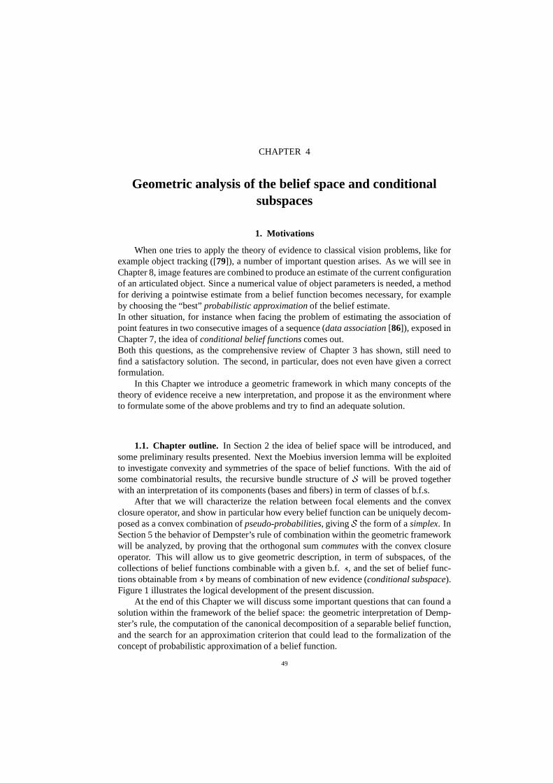
CHAPTER 4
Geometric analysis of the belief space and conditionalsubspaces
1. Motivations
When one tries to apply the theory of evidence to classical vision problems, like forexample object tracking ([79]), a number of important question arises. As we will see inChapter 8, image features are combined to produce an estimate of the current configurationof an articulated object. Since a numerical value of object parameters is needed, a methodfor deriving a pointwise estimate from a belief function becomes necessary, for exampleby choosing the “best” probabilistic approximation of the belief estimate.In other situation, for instance when facing the problem of estimating the association ofpoint features in two consecutive images of a sequence (data association [86]), exposed inChapter 7, the idea of conditional belief functions comes out.Both this questions, as the comprehensive review of Chapter 3 has shown, still need tofind a satisfactory solution. The second, in particular, does not even have given a correctformulation.
In this Chapter we introduce a geometric framework in which many concepts of thetheory of evidence receive a new interpretation, and propose it as the environment whereto formulate some of the above problems and try to find an adequate solution.
1.1. Chapter outline. In Section 2 the idea of belief space will be introduced, andsome preliminary results presented. Next the Moebius inversion lemma will be exploitedto investigate convexity and symmetries of the space of belief functions. With the aid ofsome combinatorial results, the recursive bundle structure of � will be proved togetherwith an interpretation of its components (bases and fibers) in term of classes of b.f.s.
After that we will characterize the relation between focal elements and the convexclosure operator, and show in particular how every belief function can be uniquely decom-posed as a convex combination of pseudo-probabilities, giving � the form of a simplex. InSection 5 the behavior of Dempster’s rule of combination within the geometric frameworkwill be analyzed, by proving that the orthogonal sum commutes with the convex closureoperator. This will allow us to give geometric description, in term of subspaces, of thecollections of belief functions combinable with a given b.f. � , and the set of belief func-tions obtainable from � by means of combination of new evidence (conditional subspace).Figure 1 illustrates the logical development of the present discussion.
At the end of this Chapter we will discuss some important questions that can found asolution within the framework of the belief space: the geometric interpretation of Demp-ster’s rule, the computation of the canonical decomposition of a separable belief function,and the search for an approximation criterion that could lead to the formalization of theconcept of probabilistic approximation of a belief function.
49

50 4. GEOMETRIC ANALYSIS OF THE BELIEF SPACE AND CONDITIONAL SUBSPACES
FIGURE 1. Scheme of the geometric analysis of the space of belief functions.
2. Belief space
Consider a frame of discernment � and introduce in the Euclidean space �� ����� an or-
thonormal reference frame��� � # � 6 � � � � � � � � in which, given an arbitrary ordering in ��� ,
each coordinate function� �
measures the value of belief associated to a the i-th subset of� .
DEFINITION 27. The belief space associated to � is the set of points � of �� ����� that
correspond to a belief function.
2.1. Limit simplex. The properties of Bayesian belief functions can be useful to havea first idea of the shape of the belief space.
LEMMA 1. If � is a Bayesian belief function over a frame � and� � � arbitrary,
(*) � � � �� � � � � � � � � � � � �PROOF. The sum can be rewritten as
��� � � � � � ���where
� � is the number of subsets of B containing � . But� � � � � � � � �
for each singleton,so that
(*) � � � �� � � � � � � � � ��� �� � ��� � � � � � � � �
As a consequence all the Bayesian functions are constrained to belong to a well-determinedregion of the belief space.
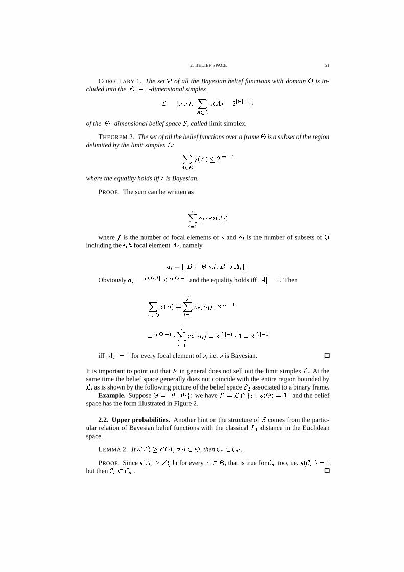
2. BELIEF SPACE 51
COROLLARY 1. The set�
of all the Bayesian belief functions with domain � is in-cluded into the
� � � � � -dimensional simplex
� � � ���� � � (*) �� � �� � � � � � � � #
of the� � � -dimensional belief space � , called limit simplex.
THEOREM 2. The set of all the belief functions over a frame � is a subset of the regiondelimited by the limit simplex
�:
(*) � �� �� %�� � � � � �
where the equality holds iff � is Bayesian.
PROOF. The sum can be written as
� � 6 �
��� ' � � � �
where�
is the number of focal elements of � and ��
is the number of subsets of �including the
��� � focal element ��, namely
�� � � � � � � ��� � � � � �
� # � �Obviously �
� � � � ��� ( � % � � � � � �
and the equality holds iff� � � ��� . Then
(*) �� � �� �
� � 6 �
' � � � � � � � � � � �
� � � � � � � �� � 6 �
' � � � � � � � � � � � � � � � � � � � �
iff� �� � ���
for every focal element of � , i.e. � is Bayesian.
It is important to point out that�
in general does not sell out the limit simplex�
. At thesame time the belief space generally does not coincide with the entire region bounded by�
, as is shown by the following picture of the belief space ��� associated to a binary frame.Example. Suppose � ��� � � �!�"�"# : we have
� � � � ��� � � � � � � # and the beliefspace has the form illustrated in Figure 2.
2.2. Upper probabilities. Another hint on the structure of � comes from the partic-ular relation of Bayesian belief functions with the classical � � distance in the Euclideanspace.
LEMMA 2. If � � �������� � �� � � � � , then+-, � +-,�� .
PROOF. Since � � �������� � �� for every ����� , that is true for+ ,��
too, i.e. � � +-,�� � ���but then
+-, � +-,�� .
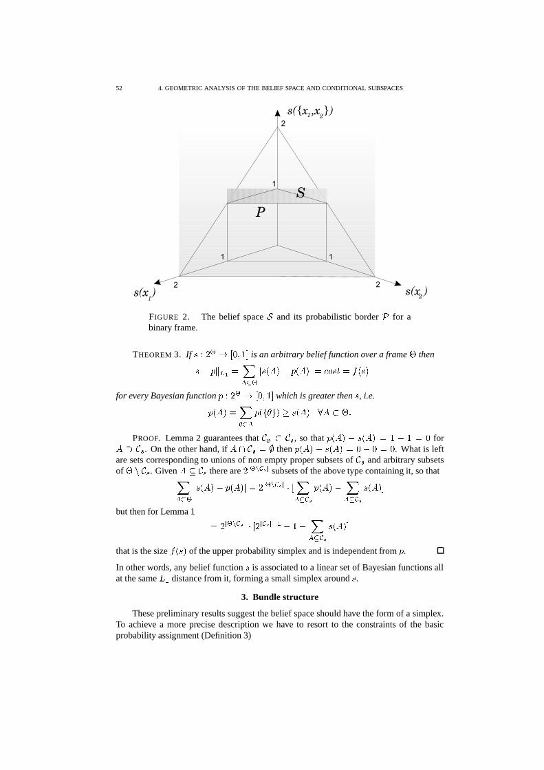
52 4. GEOMETRIC ANALYSIS OF THE BELIEF SPACE AND CONDITIONAL SUBSPACES
FIGURE 2. The belief space � and its probabilistic border�
for abinary frame.
THEOREM 3. If � ����� � � � � �"! is an arbitrary belief function over a frame � then� � ��� ��� � � (*) �� � � ������ � �� � � � � � � � � � �
for every Bayesian function � ����� � � � � �"! which is greater then � , i.e.
� � �� � ��� ( � � � � # � � � � �� � � ���&�PROOF. Lemma 2 guarantees that
+�� � +-, , so that � � ���� � � �� � � � � � � for� � +-, . On the other hand, if � + , � $
then � � ���� � � �� � � � � � � . What is leftare sets corresponding to unions of non empty proper subsets of
+3,and arbitrary subsets
of ��� +-, . Given � � +-, there are � � ����� � subsets of the above type containing it, so that
(*) �� � � �� ��� � �� � � �
� ����� � ��� (�� � �� ���� (�� � �
� �� !
but then for Lemma 1� � � ����� � ��� � � � � � � � � � (�� � �
� �� !
that is the size� � � � of the upper probability simplex and is independent from � .
In other words, any belief function � is associated to a linear set of Bayesian functions allat the same � � distance from it, forming a small simplex around � .
3. Bundle structure
These preliminary results suggest the belief space should have the form of a simplex.To achieve a more precise description we have to resort to the constraints of the basicprobability assignment (Definition 3)
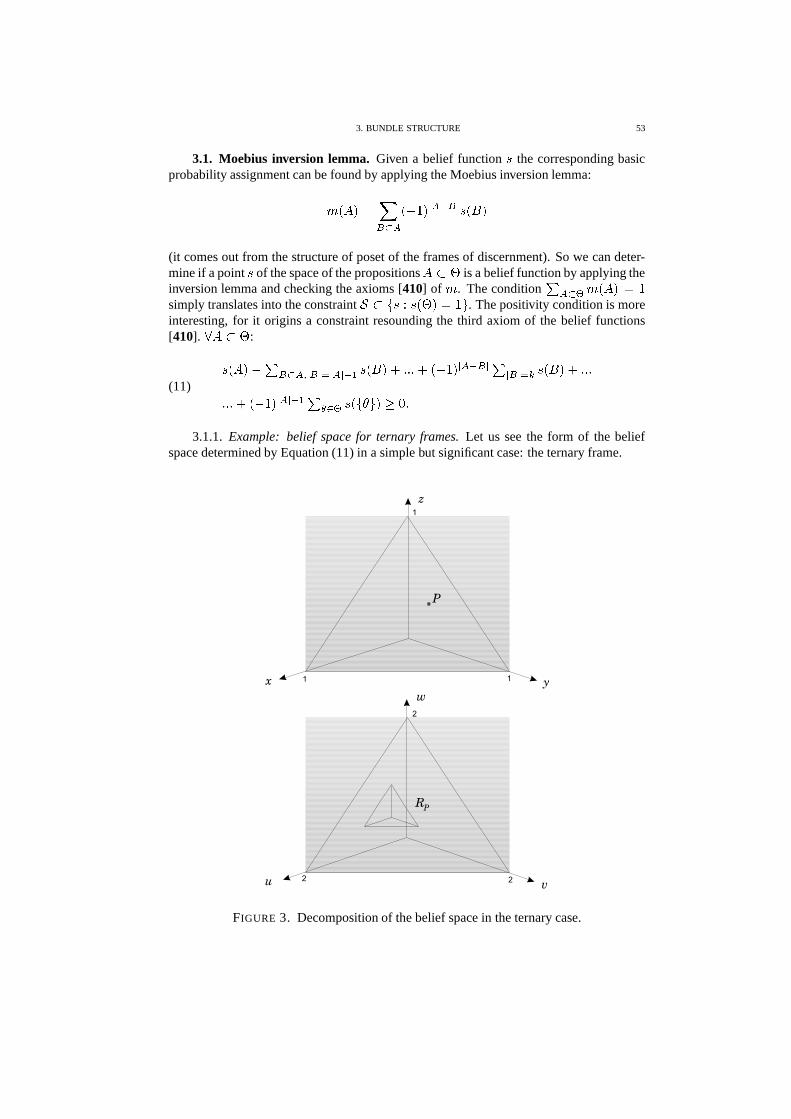
3. BUNDLE STRUCTURE 53
3.1. Moebius inversion lemma. Given a belief function � the corresponding basicprobability assignment can be found by applying the Moebius inversion lemma:
' � �� � � ) ( � � � �� (�� � � � ��� �
(it comes out from the structure of poset of the frames of discernment). So we can deter-mine if a point � of the space of the propositions � � � is a belief function by applying theinversion lemma and checking the axioms [410] of ' . The condition � (*) � ' � �� � �simply translates into the constraint � � � � ��� � � � ��� # . The positivity condition is moreinteresting, for it origins a constraint resounding the third axiom of the belief functions[410]. � � � � :
� � ���� � � ) ( � � � 6 � ( � � � � ��� � � � � � � � � � � � (�� � � � � � � 6 � � ��� � � � � �� � � � � � � � � ( � � � � ��� � � � � � # � � ���(11)
3.1.1. Example: belief space for ternary frames. Let us see the form of the beliefspace determined by Equation (11) in a simple but significant case: the ternary frame.
FIGURE 3. Decomposition of the belief space in the ternary case.

54 4. GEOMETRIC ANALYSIS OF THE BELIEF SPACE AND CONDITIONAL SUBSPACES
� �
�������������������
� � � � � � � � ��� �� � � � � � � � ��� �� � � ��� � � � ��� �� � � � � � � �� � � � ��� ��� � � �
(12)
Combining the last equation in (12) with the others we obtain
� % � ��� ��� % � � � % � � � � � % �and observe that, called
� � � ��� ���, necessary follows�� � � � % � � � � � % � � �
� � � � ��� � � � � � � ��� � ��� � � � ��� ���In other words, � reveals the structure of fiber bundle, in which the variables
� � � � � canmove freely in the unitary simplex, while the others are constrained to stay in a tetrahedron��
that depends on the sum� ��� ����� �
(see Figure 3).System (12) shows a natural symmetry that reflects the intuitive partition of the variables intwo sets, each associated to subsets of � with a same size, respectively
��� � � � � #� � � � ���and� � � � ��� # � � � � � .
It is easy to see that the group of symmetry of � is the permutation group� � � � , acting onto��� � � � � # � � � � � ��� # following the correspondence
��� ��� ��� � � ��� � �*�3.2. Convexity. Equation (11) shows that all the constraints defining � are of the
form
� � � � �� � � � � � �
�where � � and � � are two disjoint sets of variables (the above example confirms this, too).It follows immediately that
THEOREM 4. � is convex.
PROOF. Let us take two points� 7 � � �
) � and prove that all the points of the segment� 7 ��� ��� � � � 7 � �'� % � % � , belong to � .For
� 7 � � �) �
� � � � � 7� � � � � � � 7
� � � � � � ��� � � � � � �
��so that� � � � � ���� � � � � � � � � 7 � ��� � � �� � � 7 � � ! � � � � � � � 7 � ��� � � � � � � � �� � � 7 � � �
� � � � � � � � � � � � 7 � ��� � � � � � � �� � � � � � � � � � � � � 7 � ��� � � � � � � �� �� � � � � � � � 7 � ��� � � �� � � 7 � � ! � � � � � � ���� �
3. BUNDLE STRUCTURE 55
3.3. Symmetry. Let us establish for sake of simplicity the following notation:� � � � � � � � � ��� � � � � �!� � ��� � � �!����# � .
PROPOSITION 22. The general symmetry of the belief space is described by the fol-lowing logic expression�
��� � � � ���� 6 �
����
� ��� � � � � � � � # � � � ��� � � �!��# � ��� � � #� � � � � � � � � ����� � � � � � � � � � � � ����� �
PROOF. Let us rewrite the Moebius constraints, using the above notation:
� � � � � � � ��� � � � �
� 6 �
� � � � � � � � � � � � � � � ��� ) � � � � � � ���� � � � � � � � ��Looking at the right side of the inequality, it is clear that (due to its symmetry), an exchangeis possible only between variables associated to subsets of the same size.Given the triangular form of the set of constraints (the first group concerns variables ofsize 1, the second group variables of size 1 and 2, and so on), permutations among size�
variables are always induced by permutations of variables of smaller size. Hence thesymmetries of � are determined by permutations of singletons.Finally, we need to note that an exchange of singletons
� � � � �determines a series
of exchanges among the variables related to subsets containing � � and � � . The resultingsymmetry � for the
�-th group of constraints is
� � � � � � � � � � � � � � � � � � � � � � ����� � � � � � � � � � � � ����� � � �� ��� � ��� � � � � � � � # � � � ��� � � �!��# � ��� � � # �
Since � is contained into ��� � , and -� is always trivial (as a simple check confirms), theoverall symmetry is determined by � , and we have the thesis.
In other words, the symmetry of � is determined by the action of the permutationgroup
� � � � over the collection of the size 1 variables and the action of� � � � naturally
induced on the other variables
� ) � � � � � � � � � � � � � � � � � �� � � � � � � ��� �� � � � � � � �5� � ���where
� � � � � is the class of the size�
subsets of � . It is not difficult to recognize thesymmetry properties of a simplex, i.e. a collection � � � ��� � � � �-� ! of points in the Euclideanspace together with the sub-collections (faces) � �
� � ��� � � � � ��� ! of all the orders� % � .
3.4. Recursive bundle structure. One could ask if the decomposition property ob-served in the ternary case of the above example is a peculiar feature of a very simple frameor a hint of a general feature of the belief space.
LEMMA 3.
� � �
0 6 �� � � � 0 � ��� � � �' � ��� � � � � � � � � � �
� � � �� � � �� � �� � � � �&�

56 4. GEOMETRIC ANALYSIS OF THE BELIEF SPACE AND CONDITIONAL SUBSPACES
PROOF.
� � �
0 6 �
� � � � 0 � ��� � � �' � � � � � � � �� ��� � � � �
� � � � � � � � � � � � 1 � � � 2 � � � �� � �� � � � �
�� � � �� � � � � � � � � � � � � � � �� � � � � � � � � � � � � � � � 1 � � � 2 � � � � � ��� � ��� � � � � � ���� � � �� � � � � �
The first two terms of the numerator have a factor in common and can be rewritten as
� � � � �� � � � � � � � � � � � � � �this in turn has in common
� � � � � � � � � � �� � � � � � � � �with the third addendum giving� � � � � � � � � � � � ��� � � � �� � � � � � � � �
and so on. By iteration we get the thesis.
THEOREM 5.
� ( � 6 � �� ���% � � � � �
0 6 �
� � � � � � 0 � �� � � � ' � � �
� � ' � �� � � � 6 0� ��� ���(13)
PROOF. Let us suppose we have assigned an amount of mass to the subsets of sizesmaller than
�,� ' ��� � � � ��� � � # with � � � � � � ' ��� � � �
. The maximum value of� ( � � �� will correspond to giving the remaining mass� � � � ( � � � ' � �� to the subsets
of size�
. We obtain
� � � ( � � � '� �� �
��� � � � ( � � � � � ) ( � � � � � (�� � � � ��� � ��� � � � � �� ( � 6 0 6 � � 0 � � � 6 � 6 �� � � � 0 � � � ��� �
��� � � � �
� ( � 6 0 6 �
0 � � � 6 � 6 �
� � � � 0 � ��� � � �' � � � � � � � 6 � ���� �
for � � � �0 � � � is the number of subsets of size ' containing a fixed set� � � ��� � �
in a framewith n elements. This can be rewritten as
� � � � �
� � � 6 � 6 �
� � � � 6 � ���� � � �
� � �
0 6 �
� � � � 0 � ��� � � �' � ���that using Lemma 3 becomes
� � � � �
� � � 6 � 6 �
� � � � 6 � ���� � � � � � � � � � � � �
� � � �� � � �� � �� � � � �8�(14)
Now, if we write � � ( � 6 � � � �� �� � ( � 6 � � ) ( '
� �� �� � 6 �
� � � 6 � '��� � �
� � � �� � � � �
3. BUNDLE STRUCTURE 57
(since � � � �� � � � is the number of size�
subsets including size�
subsets)
� � � � 6 � '��� � �
� � �
� 6 �
� � � �� � � � � � � � � 6 � '
��� � �
� � � � 6 � '��� � �
� � �
� 6 �
� � � �� � � � ���
� 0 6 �
� � � � � � 0 � � � '� � ' � � � � 6 0� ��� � !
� � � � 6 � '��� � �
� � �
� 6 �
� � � � � � � � �� � � �� � � � � � � 6 � � ��� � �
by substituting to the first addendum Equation (14) we get
� � �� � �
� 6 �
� � � � � � � � � � � � � � 6 � ���� � � ���
� � � �� � � ��� � � � �� � � �
� � �� � � � � !and by developing the pair of binomials we have the thesis.
THEOREM 6. The belief space � has a recursive bundle structure, i.e. it can be de-composed into a sequence of domains
�� �� � � 1 � 2 � � 1 � 2 �� � � �
�� �
� ��� � � � � � � � ��� � 1 � 2 � �� � � 1 � 2 � � 1 � 2 �� � � �� � �
�� ����� � � � � � � �
� � � � � ��� � � �� � �
� 1 � � � 2 � �� �� � � 1 � � � 2 � � 1 � � � 2 �� � � �� � �
� �� � � � � � � � ��� � � � � � � � � � � � � � ��� � � � � � � � � �
where ��� � � � � � � � � � � is the section of the belief space with� � � � � � � � � � cost � � % � .� 1 � 2 is called the i-th basis of � and is defined by the following equations
��������������������������� ��������������������������
� ��� ��� � ����������������� �� ���! � �"�#�%$ & & & $ # �('�)) "�*
�%$�& & & $ * � '�,+ ������� �,+ -
�"�*�.$ & & & $ * � '/)) " � $ & & & $�0 '
� ����� � � �1 ��2�� ����3 � ������� �� ���! �54 0 �768�9�: �76
; �"�*�%$�& & & $ * �<'/)) " � $ & & & $=0 '
� ��� ��� � -
� ��� ��� � ��> ����,?@������� ?% ���! � �"�#�%$�& & & $ # �<'/)) "�*
�%$�& & & $ * ? '�,+ ����� � �,+ -
where� � � % � .� 1 � 2 is the i-th fiber of the belief space and �
�the projection map of the i-th bundle level.
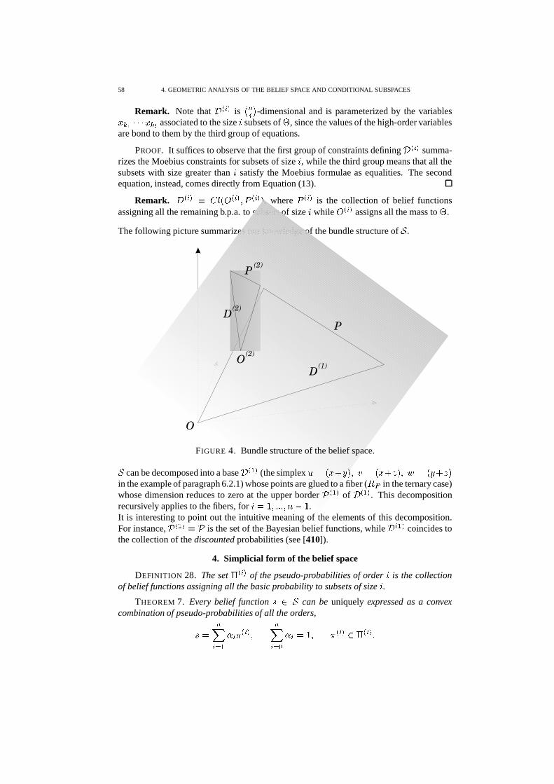
58 4. GEOMETRIC ANALYSIS OF THE BELIEF SPACE AND CONDITIONAL SUBSPACES
Remark. Note that� 1 � 2 is � � � � -dimensional and is parameterized by the variables� � � � � � � � associated to the size
�subsets of � , since the values of the high-order variables
are bond to them by the third group of equations.
PROOF. It suffices to observe that the first group of constraints defining� 1 � 2 summa-
rizes the Moebius constraints for subsets of size�, while the third group means that all the
subsets with size greater than�
satisfy the Moebius formulae as equalities. The secondequation, instead, comes directly from Equation (13).
Remark. � 1 � 2 �� � ��� 1 � 2 � � 1 � 2 � , where
� 1 � 2 is the collection of belief functionsassigning all the remaining b.p.a. to subsets of size
�while
� 1 � 2 assigns all the mass to � .
The following picture summarizes our knowledge of the bundle structure of � .
FIGURE 4. Bundle structure of the belief space.
� can be decomposed into a base� 1 � 2
(the simplex � � � � ��� � � � � � � � � � � � � � � � � �in the example of paragraph 6.2.1) whose points are glued to a fiber (
� �in the ternary case)
whose dimension reduces to zero at the upper border� 1 � 2
of� 1 � 2
. This decompositionrecursively applies to the fibers, for
� � � ��� � � �!� � � .It is interesting to point out the intuitive meaning of the elements of this decomposition.For instance,
� 1 � 2 � �is the set of the Bayesian belief functions, while
� 1 � 2coincides to
the collection of the discounted probabilities (see [410]).
4. Simplicial form of the belief space
DEFINITION 28. The set �81 � 2 of the pseudo-probabilities of order�
is the collectionof belief functions assigning all the basic probability to subsets of size
�.
THEOREM 7. Every belief function � ) � can be uniquely expressed as a convexcombination of pseudo-probabilities of all the orders,
� � � � 6 �
� ��� 1 � 2 � � � 637 �� ��� � � 1 � 2 ) � 1
� 2 �
4. SIMPLICIAL FORM OF THE BELIEF SPACE 59
PROOF.
� � � � ) ( ' ��� � �'����� � � � � 6 �
� � ) ( � � � 6 �' ��� � � � � � �
but then� 1 � 2 �� � � ) ( � � � 6 �
' ��� � �'����� �is an unnormalized belief function assigning all the mass to subsets of size
�.
If we define� 1 � 2 �� � 1 � 2� � 1 � 2 �
we can write
� � � � 6 �
� � 1 � 2 � � 1 � 2 � � � 6 �
� � � 1 � 2with � �� 6 �
� � � � �� 6 �
� � 1 � 2 � � � for the normalization constraint. Obviously� 1 � 2 )
� 1 � 2 .It is interesting to note that �81 � 2 � � 1 � 27 .This convex decomposition property can be easily generalized in the following way.
THEOREM 8. The set of all the belief functions with focal elements in a certain col-lection
�is closed and convex in � , namely� � ��� ) ��, � � ) � # �
� � � � � ( ��� ) � # �where
� ( is the pseudo-probability assigning all the mass to � , ' ���'� �� � � .PROOF. By definition
� � ��� ) �-, � � ) � # �� � � � � � ) ( � �
' ��� � � � ��, � � #but
� � � � ' ��� � � � � ( ��� � � � �
�� ( � � � � �� � �
but� � ( ��� � � � �
�� ( � � � � �� � � �� � � �
so that
� � � � ' ��� � � � � � ��� ' ��� � � �
by extending ' to the elements� ) � � � � as ' ��� � � � . Since ' is a basic probability
assignment, � � ��� ' ��� � � � and the thesis follows.
COROLLARY 2. � 1 � 2 �� � � � � � � � ��� � � # � .
COROLLARY 3. The belief space � coincides to the convex closure of all the pseudo-probabilities of every order,
� �� � � � � ��� � � � � � � � � � � �
� � ��� �
� ��� � � � � �� ��� � � � � � � �� � � ���(15)

60 4. GEOMETRIC ANALYSIS OF THE BELIEF SPACE AND CONDITIONAL SUBSPACES
The above result (that can be obtained directly from Theorem 8) confirms our conjec-ture about the nature of simplex of the belief space, rising from the symmetry analysis ofParagraph 3.3.
5. Commutativity
THEOREM 9.+
l and � commute, i.e. if � is combinable with � � � � � ��� ��� � � �!� then
� �� � � � � � #���� � � � � �$�-# � �
� � � � � � � � #���� � � � � � � �$� # � �in other words
� � -� � � � � � �� � � � � � � � � � -� � � ��� �
Remark. Note that � operates over ��� � � ��� � � � �$� as belief functions while Cl operatesover points of the belief space as a Euclidean space: this claim is meaningful only in thecontext of the belief space.
Remark. Being � convex, if � � ) � � � then � � � � � � ) � when � � � � � � .PROOF. Let us first compute the basic probability assignment associated to � � � � � � .
It suffices to use the Moebius inversion formula
' � �� � � ) ( � � � �� (�� � � � ��� ���
If by hypothesis � ��� � � � � � � � � ��� � then
'�� � , � �� � � � ) ( � � � � � (�� � � � � � � � � ��� � �� � � � � � � ) ( � � � � � (�� � � � � ��� � � � � � � ' � � ����
Now, being � � � � � � ) � for the above remark, we must check if it combinable with withs, obtaining � � � � � � � � . Called
��,the collection of focal elements of a belief function � ,
we have� � � , � .� / � 54637
��, �(16)
if� � �� � � � this reduces to
� � � , ��� ��, . This way if � is combinable with some � �(even only one of them) then it is combinable with � � � � � � .Let us call � � ��� � � � �� the focal elements of � � � � � � and
�� ��� � � � � 0 those of � . The focal
elements of � � � � � � � � are
. � ��,�� , for all the intersections are considered, but property 16 gives exactly the same result forthe f.e. of � � � � � � � � � � .Finally we have to check the corresponding basic probability assignments: for the latter
6. CONDITIONAL SUBSPACES 61
we have, denoting with� ����# the focal elements of � � ,'�� � ,�� , � �� �
� � ) ( � � � �� (�� � � �� � � � � � � � � ��� � � �� � � � ) ( � � � �
� (�� � � � � � � � � ��� �
� � � � � ' ,�� , � �� � � � � � �� � � � 6 ( ' , � ��� � ' , ��� � �
� � �� � � � 6�� ' , � ��� � ' , ��� � �
while for � � � � � � � �
6 ����� �� � � � � >�
��� � 3 6 � �� � � � ��6 � � ? �
� � ���� � 3�� 6 � �� � � � ��6 � � ? �
>�
��� � 3 � � � � � 6 � � � ��� � 6 � � ? �
� � ���� � 3�� � � � � � 6 � � � ��� � 6 � � ? �
>� � � � � �
��� � 3 6 � � � ��6 � � ? �� � � � � �
��� � 3�� � � � � � 6 � � � ��� � 6 � � ? �
>� � � � � �
��� � 3 6 � � � ��6 � � ? �� � � � � ����� ���� � 3�� 6 � � � ��6 � � ? ���
> � � � � � � ��� � 3 6 � � � ��6 � � ? �� � � ��� � 3�� 6 � � � ��6 � � ? �
&Since for ��� �) ��, the addenda vanish, we remain for each
�with the focal elements of� � :
�� � � � � �� � � � 6 ( ' , � ����� ' , ��� � �
� � � �� � � � 6�� ' , � ��� � ' , ��� � � � ��� ) ��, �
The fact that orthogonal sum and convex closure commute is a powerful tool, providing usa simple language for giving geometric interpretations to the notion of combinability andconditioning.
6. Conditional subspaces
DEFINITION 29. The conditional subspace � � � is the set of the belief functions condi-tioned by a given function � , namely
� � � �� � � � � � � ) � ��� � � � � � � #(17)
Since not every belief function is combinable with an arbitrary � , we need to investigatethe geometric structure of combinable functions.
DEFINITION 30. The non-combinable subspace ��� � � associated to a belief func-
tion � is the collection of all the b.f.s that are not combinable with � ,��� � � �� � � � � � ��� � � ��#��
62 4. GEOMETRIC ANALYSIS OF THE BELIEF SPACE AND CONDITIONAL SUBSPACES
PROPOSITION 23. ��� � � �
� � � � � ( ��� +-, � $ # � .PROOF. It suffices to point out that �
�� � � � � ��� � +-,�� � + , # � � ��� ����� + , � � )+ , � # . Hence we can apply Theorem 8 and the thesis follows.
The dimension of ��� � � is obviously � � ����� � � � .
Using the definition of non-combinable subspace we can write � � � � � � � � � ��� � � � �� � � ��� � +-,�� +-, �� $ # . Unfortunately, the last expression does not seem to satisfy Theorem
8: for a b.f. ��� to be compatible with � it suffices to have one focal element intersecting thecore+-,
, not all of them.
DEFINITION 31. The compatible subspace
�� � � associated to a belief function � is
the collection of all the b.f.s with focal elements included into the core of � :�� � � �� � ��� �+-,�� � +-, # .
From Theorem 8 it follows
COROLLARY 4.
�� � � �
� � � � � ( ��� � +-, # � .The compatible space
�� � � is only a proper subsets of the set of belief functions combin-
able with � , � � ��� � � : nevertheless, it contains all the relevant information.
THEOREM 10. � � � � � ��� � � .
PROOF. Let us denote with�-,�� � � � � # and
��, � � � � # the focal elements of ��� and �respectively. Obviously
� � �� � � � �
� +-, � � � �� �� +-, � so that defining a new
b.f. � � � with focal elements
� � �� �� +-,
and basic probability assignment
' � � � � � � � ' � � � � �we have � � ��� � � � � � � .Now we can find a geometric description of the conditional subspace. From Theorem 8and 10 it follows that
COROLLARY 5. � � � �� � � � � � � ( � � � +-, # � .
Note that � � �� � � and then � is always a vertex of � � � .
Of course � � � ��� � � , since the core is a monotone function on the poset
� � ��� � � . Fur-thermore
� � ' � � � � � � � � � � � �(18)
for the dimension of � � � is simply the cardinality of
�� � � (note that
$is not included)
minus 1.We can observe that
� � ' � � � � � � � � � � ' � � � � � �� � � ' � � ���
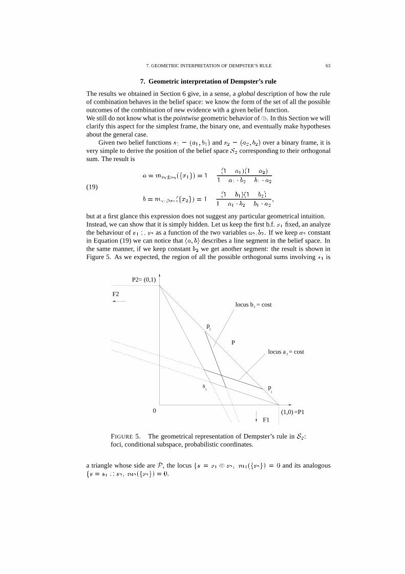
7. GEOMETRIC INTERPRETATION OF DEMPSTER’S RULE 63
7. Geometric interpretation of Dempster’s rule
The results we obtained in Section 6 give, in a sense, a global description of how the ruleof combination behaves in the belief space: we know the form of the set of all the possibleoutcomes of the combination of new evidence with a given belief function.We still do not know what is the pointwise geometric behavior of � . In this Section we willclarify this aspect for the simplest frame, the binary one, and eventually make hypothesesabout the general case.
Given two belief functions � �� � � � ��� � � and �$� � � � ������� � over a binary frame, it is
very simple to derive the position of the belief space ��� corresponding to their orthogonalsum. The result is
� � ' , � � , � � ��� � # � ��� � � � � � � � � � � � � �� � � � ��������� � ��� �
� � ' , � � , � � ��� �"# � ��� � � � ��� � � � � ����� �� � � � ��������� � � � � �
(19)
but at a first glance this expression does not suggest any particular geometrical intuition.Instead, we can show that it is simply hidden. Let us keep the first b.f. � � fixed, an analyzethe behaviour of � � � �$� as a function of the two variables � � ����� . If we keep � � constantin Equation (19) we can notice that
� � ���"� describes a line segment in the belief space. Inthe same manner, if we keep constant ��� we get another segment: the result is shown inFigure 5. As we expected, the region of all the possible orthogonal sums involving � � is
(0,1)
(1,0)0
F2
F1
P2=
=P1
s p
p2
11
P
locus b = cost
locus a = cost
2
2
FIGURE 5. The geometrical representation of Dempster’s rule in ��� :foci, conditional subspace, probabilistic coordinates.
a triangle whose side are�
, the locus� � � � � � �$��� ' �
� � �$�"# � � � and its analogous� � � � � � �$��� ' � � � �$�"# � � � .
64 4. GEOMETRIC ANALYSIS OF THE BELIEF SPACE AND CONDITIONAL SUBSPACES
In other words, the subset of belief functions obtainable from � � by combination of addi-tional evidence is
� � �� �
� � � � � � � � � � �� � � � � � �"# � �
� � � � � � � � � � ��� � � � � � � # �confirming the geometrical structure of the conditional subspace.
7.1. Foci of the conditional subspace. Subsets corresponding to sums � � � �$� with' �� � �$�"# � � � � � are intersections of lines all exiting from a point � � outside the belief
space with the above triangle. In a dual way, the sums � � � �$� with ' � � � �$�"# � � � � � lieeach on a different line passing through another point � � .We can get their coordinates by simply intersecting the line passing through
� � � � � and� � ���"� with the line� � �
:
� �� � � ��� ' , � � � �' , � � ��� � # � � �*� � � � ' , � � � �' , � � ��� �"# � � � ���(20)
We call them foci of the conditional subspace generated by �"� (see Figure 5 again). Obvi-ously from Equations (20)
PROPOSITION 24.� � � , � 7 � � � � .
while
PROPOSITION 25.� � � , � � � ��� � � � � �
.
In other words, simple probabilities can be seen as foci of the probabilistic conditionalsubspace
�.
7.2. Probabilistic coordinates of conditional belief functions. It is interesting tonote that each point of the conditional subspace is uniquely associated to a pair of proba-bilities, more precisely the intersections of the generator lines
��� � � � and
� � � �*� � withthe probability subspace
�:
� ��� �
� � � � �� � � � �(21)
DEFINITION 32. We call � � and � � probabilistic coordinates of the conditional belieffunction � � , � ) � � �
�.
In this simple 2-dimensional case, we can calculate their explicit form by exploiting thedefinition, obtaining for � �
� �� � 1 � ��� � ��� � 2 1 � ��� � 2 1 � ��� � 21 � ��� � 2 1 � ��� � ��� � � � 2 ��� � 1 � ��� � 2 1 � ��� � 2� �� ��� ��� �� � � � 1 � ��� � ��� � 2 1 � ��� � 21 � ��� � 2 1 � ��� � ��� � � � 2 ��� � 1 � ��� � 2 1 � ��� � 2 �
(22)
similar expressions can be derived for � � .Summarizing, given a belief function �"� ) � � the orthogonal sum � � � �$� for any b.f.� �� � �
� � � � � is the unique intersection of the pair of lines�
��� � � � � and
� � �� �*� � �� � � �$� � � �
� �where � �
� � �� �
� � and � � � � � � � � � .The probabilistic coordinates have some remarkable properties.
PROPOSITION 26. If � �) �
then � �� � � � � � � �$� ) �
(it suffices to look at Figure 5), and
PROPOSITION 27. � �� �
� � � � � � � � � � � .
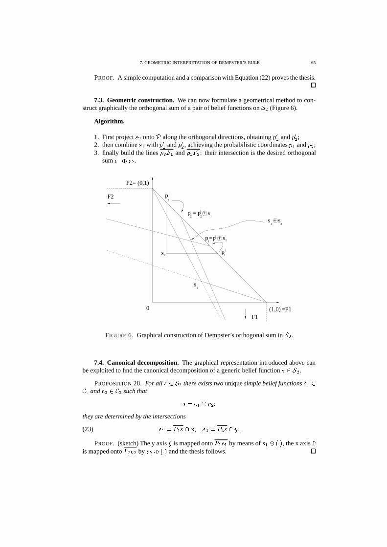
7. GEOMETRIC INTERPRETATION OF DEMPSTER’S RULE 65
PROOF. A simple computation and a comparison with Equation (22) proves the thesis.
7.3. Geometric construction. We can now formulate a geometrical method to con-struct graphically the orthogonal sum of a pair of belief functions on � � (Figure 6).
Algorithm.
1. First project � � onto�
along the orthogonal directions, obtaining � � � and � �� ;2. then combine � � with � � � and � �� , achieving the probabilistic coordinates � � and � � ;3. finally build the lines � � � � and � � �*� : their intersection is the desired orthogonal
sum � � � �$� .(0,1)
(1,0)0
F2
F1
P2=
=P1
s1
s2p
1
p2
|
|
1
1
2s + s
+ sp2
|p2=
1
+ sp|
1p= 1
FIGURE 6. Graphical construction of Dempster’s orthogonal sum in � � .
7.4. Canonical decomposition. The graphical representation introduced above canbe exploited to find the canonical decomposition of a generic belief function � ) � � .
PROPOSITION 28. For all � ) �*� there exists two unique simple belief functions�
�)+
� and� � ) + � such that
� � � � � � � �they are determined by the intersections�
�� �
� � ��� � � � � � � � ��� �(23)
PROOF. (sketch) The y axis��
is mapped onto�
��
� by means of � � � � � � , the x axis��
is mapped onto� � � � by �$� � � � � and the thesis follows.
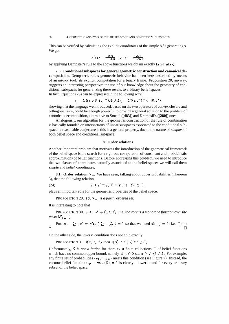
66 4. GEOMETRIC ANALYSIS OF THE BELIEF SPACE AND CONDITIONAL SUBSPACES
This can be verified by calculating the explicit coordinates of the simple b.f.s generating s.We get
� ��� � � � 1 , 2� � � 1 , 2 � �� � � � � 1 , 2� � � 1 , 2 �
by applying Dempster’s rule to the above functions we obtain exactly� � � � � � � � � � � .
7.5. Conditional subspaces for general geometric construction and canonical de-composition. Dempster’s rule’s geometric behavior has been here described by meansof an ad-hoc tool: its explicit computation for a binary frame. Proposition 28, anyway,suggests an interesting perspective: the use of our knowledge about the geometry of con-ditional subspaces for generalizing these results to arbitrary belief spaces.In fact, Equation (23) can be expressed in the following way:� � � � � � ��� � � � � �
� � � � � � � � � � � � ��� � � � � � � � � � � �showing that the language we introduced, based on the two operators of convex closure andorthogonal sum, could be enough powerful to provide a general solution to the problem ofcanonical decomposition, alternative to Smets’ ([483]) and Kramosil’s ([280]) ones.
Analogously, our algorithm for the geometric construction of the rule of combinationis basically founded on intersections of linear subspaces associated to the conditional sub-space: a reasonable conjecture is this is a general property, due to the nature of simplex ofboth belief space and conditional subspace.
8. Order relations
Another important problem that motivates the introduction of the geometrical frameworkof the belief space is the search for a rigorous computation of consonant and probabilisticapproximations of belief functions. Before addressing this problem, we need to introducethe two classes of coordinates naturally associated to the belief space: we will call themsimple and belief coordinates.
8.1. Order relation �� . We have seen, talking about upper probabilities (Theorem3), that the following relation
� ��� � � � � �� ��� � � �� � � ���&�(24)
plays an important role for the geometric properties of the belief space.
PROPOSITION 29.� � ����'� is a partly ordered set.
It is interesting to note that
PROPOSITION 30. � �� ��� � +-, � +-,�� , i.e. the core is a monotone function over theposet
� � ��� �'� .PROOF. � � � � � � � � +-, � � � � � � +-, � � � � so that we need � � + , � � � � , i.e.
+-, � �+-,.
On the other side, the inverse condition does not hold exactly:
PROPOSITION 31. if+ , � +-, � then � � �� ��� � � �� � � � +-, �
Unfortunately, � is not a lattice for there exist finite collections � of belief functionswhich have no common upper bound, namely
� � � ) � s.t. �� � � � ) � . For example,any finite set of probabilities
� � � ��� � � ��� ��# meets this condition (see Figure 7). Instead, thevacuous belief function � � � ' 7 � � � � � � is clearly a lower bound for every arbitrarysubset of the belief space.
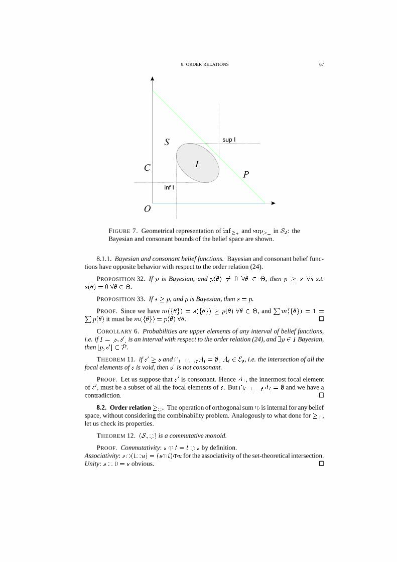
8. ORDER RELATIONS 67
FIGURE 7. Geometrical representation of � ������� and ����� ��� in � � : theBayesian and consonant bounds of the belief space are shown.
8.1.1. Bayesian and consonant belief functions. Bayesian and consonant belief func-tions have opposite behavior with respect to the order relation (24).
PROPOSITION 32. If � is Bayesian, and � � ��� �� � � � ) � , then � � � � � s.t.� � ��� � ��� � ) � .
PROPOSITION 33. If � � � , and � is Bayesian, then � � � .
PROOF. Since we have ' � � � # � � � � � � # � � � � ��� � � ) � , and � ' � � � # � � � �� � � ��� it must be ' � � � # � � � � ����� � .COROLLARY 6. Probabilities are upper elements of any interval of belief functions,
i.e. if � � � ��� � � ! is an interval with respect to the order relation (24), and � � ) � Bayesian,then � � � ��� ! � � .
THEOREM 11. if ���3��� and � 6 � � � � � �
� � $ �'�� ) ��,
, i.e. the intersection of all thefocal elements of � is void, then � � is not consonant.
PROOF. Let us suppose that ��� is consonant. Hence � � , the innermost focal elementof ��� , must be a subset of all the focal elements of � . But
� 6 � � � � � �� � $
and we have acontradiction.
8.2. Order relation � � . The operation of orthogonal sum � is internal for any beliefspace, without considering the combinability problem. Analogously to what done for � � ,let us check its properties.
THEOREM 12.� � � � � is a commutative monoid.
PROOF. Commutativity: � � � � � � � by definition.Associativity: � � � � � � � � � � � � � � � for the associativity of the set-theoretical intersection.Unity: � � �� � � obvious.
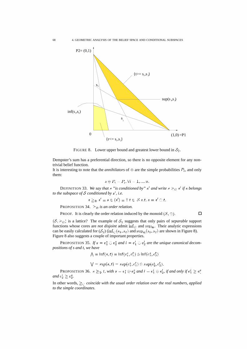
68 4. GEOMETRIC ANALYSIS OF THE BELIEF SPACE AND CONDITIONAL SUBSPACES
(0,1)
(1,0)0
P2=
=P1
s1
s2
inf(s ,s )
sup(s ,s )1 2
21
{t>= s ,s }1 2
{r<= s ,s }1 2
FIGURE 8. Lower upper bound and greatest lower bound in ��� .Dempster’s sum has a preferential direction, so there is no opposite element for any non-trivial belief function.It is interesting to note that the annihilators of � are the simple probabilities
� �, and only
them:
� � � � � � � � � � ��� ��� � � �!� �DEFINITION 33. We say that � ”is conditioned by” � � and write �8� � � � if � belongs
to the subspace of � conditioned by ��� , i.e.
� � � � � � � ) � � � � � � � ) � ��� � ��� � � � � � �PROPOSITION 34. � � is an order relation.
PROOF. It is clearly the order relation induced by the monoid� � � � � .
� � ��� � � is a lattice? The example of �*� suggests that only pairs of separable supportfunctions whose cores are not disjoint admit � ��� � and ����� � . Their analytic expressionscan be easily calculated for ( �*� ) ( � ��� � � � � � �$� � and ����� � � � � � �$� � are shown in Figure 8).Figure 8 also suggests a couple of important properties.
PROPOSITION 35. If � � � , � � � ,� and��� � �
� � � � � are the unique canonical decom-positions of s and t, we have
� � � ��� � ��� � � � � ��� �� , � � � � � � � � ��� �� ,� � � � � �� � ����� � ��� � � � ����� �� , � � � � � � � ����� �� ,� � � � � ���
PROPOSITION 36. �&� � � , with � � � , � � � ,� and��� � �
� � � � � , if and only if� �
� � � , �and
� � � � � ,� .In other words, � � coincide with the usual order relation over the real numbers, appliedto the simple coordinates.
9. PROBABILISTIC APPROXIMATIONS 69
8.2.1. Bayesian belief functions.
PROPOSITION 37. Probabilities are upper elements of any interval of belief functionswith respect to � � , i.e. if � � � ��� ��� ! is an interval with respect to the order relation � � ,and � ) � is a Bayesian belief function, then � � � � .
PROOF.
8.3. Simple and belief coordinates. Proposition 36 together with the trivially re-mark that �� � � � ( � � ( for all � � � establishes an elegant correlation betweenwhat we call belief and simple coordinates and � � , � � , respectively. This parallelism issummarized in the following table:
simple coordinates� ( Cartesian coordinates
� (� � � � � � ( � � � � � ( � � � ��� � � � � � � � � ( � � � � � ( � � � � � � �� ��� � � ��� � � � � � � ��� �� ( � � ( � � � �� � ��� � � ��� � � � � � � ��� � � ( � � ( � � � ��
9. Probabilistic approximations
As we mentioned at the beginning of this Chapter, one of the major drawbacks of the evi-dential formalism is the lack of the concept of momentum of a belief function, preventingthe foundation of an estimation framework based on conditional expectations as it exists inthe classical theory.In this final part, we investigate the possibility of exploiting the geometrical properties ofthe belief space in order to approximate, according to a criterion to be established, a givenbelief function with a finite probability (Bayesian b.f.).
9.1. Conditions. We first need to choose a suitable approximation criterion in thebelief space. It has to satisfy some intuitive conditions:
# the result ought not to depend on the choice of a particular distance function in thebelief space;# it has to produce a single pointwise approximation, and not a whole set of optimalpoints;# the criterion must be meaningful, i.e. it has to be a necessary consequence of thenature of the belief functions.
In the last Section we have learned that not every belief function has simple coordinates,and furthermore even choosing a separable support function all the probabilities � ) �
areequally distant from it. Hence, no distance function based on simple coordinates is suitableto compute the probabilistic approximation.
70 4. GEOMETRIC ANALYSIS OF THE BELIEF SPACE AND CONDITIONAL SUBSPACES
Once established the use of belief coordinates, we still have to choose a particulardistance function over them. For instance
� � ��� ��� � � (*) �� � � ��*��� � �� �
� � ��� ��� � ��� (*) � � � � ��*��� � �� � �� � ��� ����� � �����(*) �
� � � ������ � �� � �(25)
When we introduced the upper probabilities (Theorem 3) we have seen that each belieffunction � corresponds to a whole subset of Bayesian functions, which have the same(minimum) � � distance from � . This means that it cannot be used in an admissible approx-imation algorithm.
9.2. External behaviour and approximation criterion. On the other side, thereseems to be no justification for the choice of any the above distances.A brief consideration can help us. The reason of existence of the theory of evidence is therule of combination: a belief function is useful only when it is combined with others in anautomated reasoning process. That is to say, the important aspect is the external behaviorof the desired approximation: a good approximation, when combined with any other belieffunction, produces results similar to what obtained by combining the original function.Analytically,
�� � ����� � � �, � � �� � �� 1 , 2 � � � � � � � � � � � � � � � �(26)
where � � � � is one of the distance functions in Cartesian coordinates (25), and+
is the classof belief functions where the approximation must belong.
9.3. Probabilistic approximation in �*� . Let us see how this criterion works for thebinary frame.First of all, intuition suggests a slight simplification.
Conjecture. In order to compute a probabilistic approximation, it suffices to measurethe integral distance only for the probabilistic subset of
�� � � , �
�� � � , namely
�� � ����� � � �� ��� � � ��� � 1 , 2 � � � � � � � � ��� � � � � � �(27)
Of course for the binary frame the compatible subset coincides with the whole belief spacefor every belief function, so that
� �� � � � � � � ) �*� .
We get a very interesting result.
THEOREM 13. For every belief function � ) �*� , the probabilistic approximation in-duced by the cost function (27) is unique, and corresponds to the normalized plausibilityof singletons independently from the choice of the distance function � � � � .
9. PROBABILISTIC APPROXIMATIONS 71
PROOF. Using the analytic expression (19) of Dempster’s rule in ��� , given � �� � � � � � � and � � � � � � � �� , � � ��� � � � � � we get
� � � ��� � � �� � � � � �� ��� � �
� � � � � �� � � � � ��� � � � � � �� � � � � � � � � � � � � � � � � � ��� � � �
� � � � � ��� � � �� ��
� ��� �� � � � � �� � �
� �� � � � � �
� � � � � �*� � � � � � �� � � � � � � � � � � � � � � � �
since both � � � and � � � belong to�
, the line � �� � � � � , and then their difference is
proportional to� � ��� � � . By applying the cost function (27),
� �
7 � � � � ��� � � �� �� � �
� ��� � � � � � � �� � � � � ��� � � � � � � � � � � �
7 � � � � � � �� � � �� �"� � � � � � � � � � � � � � � � ! �
�� �
� ��� � � � � � � �� � � � � ��� � � � � � � � � ��� � � � � � � � � ��� � � ���
But then, � ��� �� � for every
�, since its argument is strictly positive for
� ) � � � � � .Instead, � �
�� goes to zeros for� � � � � �
� � � � � ��� � � � � � � � � �� � � � � �
� � � �� � � � �
that means
�� � � � � � �� � � �
� � � � � �� � � �
� � � �� � � � � ���
Looking at Equation (2) of Chapter 2, we can recognize the probability function�� � � �
obtained by assigning as basic probability values the normalized plausibilities of single-tons.
It is amazing to note that�� � � � � ����� � � �� ��� � � ��� � � �
i.e. the normalized plausibility�� � � � is also the unique probability that minimizes the
standard quadratic distance in the Euclidean space.
9.4. Interpretation of relative plausibilities. The following result gives us a hint ofthe meaning of the relative plausibilities of singletons.
THEOREM 14. The distance between a given generic b.f. s over a frame � and theunnormalized Bayesian belief function p obtained by choosing the plausibilities of thesingletons due to s as basic probability assignment for the elements in p' � � � � # � � � � , � � � # � ��� � � � ��� � � # �measures exactly the maximum deviation of � from the additivity rule over the singletons,namely � � � � � � �������� �
� � � � � ��� � � # �*� � � � � # � � �
72 4. GEOMETRIC ANALYSIS OF THE BELIEF SPACE AND CONDITIONAL SUBSPACES
PROOF. It suffices to prove that if � satisfies the hypothesis
������ ( 6 � � � � ���� � � �� � % ������ ( 6 � � �
� � � ���� � � �� �so that � � � � � � ������ ( 6 �
� � � ���� � � �� � � �������� �� � � � � # �*� � � � � # � � �
� �������� �� � � � � � # � � � � � � # � � � �������� �
� � � � � ��� � � # �*� � � � � # � � �If � � � � � � �'� � ��� � � � ��� � � �!����# we have
� � � ���� � � �� � � � � � � � 6 �
� � � � ��� � � ��� � � � ��� � � �!����# � �
� � � � 6 �
� � � � � � � # �*� � � � � �*� � � ��� � � � ��� � � �!����# � �
� � � � 6 �
� � ) ��� � � ' ��� � ��� � � � � �*�
� ) ��� � � � � � � � � ' ��� � �
� � � � 6 �
� � ) �' ��� ��� � ��� ' ��� � ��� � � � � � �
� ) �' ��� �*�
� ) ��� � � � � � � � � ' ��� � �
� � � ) �' ��� �*� � � 6 �
� ��� ' ��� �*� � ) �' ��� � �
� � � � � � � � � � 46�� ' ��� � �
� � � � � � � ��� � � � � � � � � ' ��� � � � � � ��� �
� � 6 �
� � ��� ��� � � � � 46 � � 54��� ' ��� � � � � �
� � � � � � � � � � � � ����� � 6 �
� � ��� ��� � � � � 46 � � � � � ����� � � � � � � � ��� � 4��� ' ��� �
so that
������ ( 6 � � � � � � ���� � � �� � �
� � � � � � � ��� � �� � � � � �� � ' ��� � � � � � ��� �
� � 6 �
�� � ��� ��� � � � � 46 � �� 54��� ' ��� � � � � �
� � � � � � � � � � � � ����� � 6 �
�� � ��� ��� � � � � 46 � � � � � ����� � �� � � � � �� ��� � 4��� ' ��� � %
10. COMMENTS 73
and defining� � �� �� � � � ��� ��� � � � � � ��� �
�� ����� �
% � � � � � � ��� ��� � � � � � � ' ��� � � � � � � ��� �
� � 6 �
� � ��� ��� � � � � 46 � � 54��� ' ��� � � � � �
� � � � � � � � � � � � ����� � 6 �
� � ��� ��� � � � � 46 � � � � � ����� � � � � � � � ��� � 4��� ' ��� � �
� ��� ���� � � � � � � � � ' ��� � �
� � 6 �
� � ��� ��� � � ��� �
� 46 � � 4��� '��� � � � � �
� � � � � � � � � � ��� 6 �
� � ��� ��� � � ��� �
� 46 � � � � � ��� � � � � � � � 4��� ' ��� � �
�� � ��� � �� � � � � � � � � ' ��� � � � � � � � � � ���
�
� 6 �
� � ��� ��� � � ��� �
� 46 � � 4��� '��� � � � � �
� � � � � � ��� �
� � � � � ��� 6 �
� � ��� ��� � � ��� �
� 46 � � � � � ��� � � � � � � � 4��� ' ��� � �
� � � � ���� � � �� � ( 6 ��� ��� � � � � � � � � � � � � ���� � � �� � ( 6 ��� � �� � � � � �� � � � � � %% ������ ( 6 � � 1 ��� � 2 � � � ���� � � �� � �
10. Comments
The reader will easily appreciate that, even if these results are not conclusive, they appearto confirm the goodness of our criteria. Some simple computations about consonant ap-proximations confirm the independence of the outcome from the chosen distance function,and its equality to what obtained by minimizing the standard quadratic distance.On the other side, the geometric description of conditional subspaces promises to be thesuitable tool for a definitive solution of problems like canonical decomposition and geo-metric construction of Dempster’s rule, perhaps providing also a quantitative measure ofthe distance from separability of an arbitrary b.f.

74 4. GEOMETRIC ANALYSIS OF THE BELIEF SPACE AND CONDITIONAL SUBSPACES
CHAPTER 5
Algebraic structure of the families of compatible frames
Together with the nature of belief functions as set-valued measures, that we analyzedin its geometrical implications in Chapter 4, the other major concept of theory of evidence,as we have learnt in Chapter 2, is the formalization of the idea of structured collection ofrepresentations of the external world encoded into the notion of family of frames.
As Equation 8 clearly shows, the concept of independence of frames resounds the ideaof independent vectors of a linear space:
� �� � � � � � � ��� � �� � �� $ � � � �
� � � � � ��� �� � � � �� ) �
We now want to demonstrate that this is more than a simple analogy: it is the symptom ofa deeper similarity of these structure at the algebraic level. Not much work has been donealong this path; in [430] can be found an analysis of the collections of partitions of a givenframe in the context of hierarchical representation of belief.
In this Chapter we will expose a complete analysis of general families of frames, notintended as partition of a common frame, but as objects obeying the small number of ruleswe have seen in Definition 14. We will distinguish among finite and general families andintroduce the new internal operation of maximal coarsening originating the structure ofsemimodular lattice.
In the next one, we will show the equivalence between internal independence offrames as Boolean sub-algebras and external independence of frames as elements of alocally finite Birkhoff lattice, and eventually propose a solution to the conflict problembased on a generalized Gram-Schmidt algorithm.
1. Motivations: measurement conflict
Belief functions carrying distinct pieces of evidence are combined by using the Dempster’srule to fuse their information and make decisions. Unfortunately, the following theoremshows that the combination is guaranteed only for trivially interacting feature spaces.
THEOREM 15. Let � � ��� � � ��� � a set of compatible FODs. Then the following condi-tions are equivalent:
1. all the possible collections of belief functions � � ��� � � � �$� defined respectively over� � ��� � � ��� � are combinable over their minimal refinement � ��� � � � � � � �2. � � ��� � � ��� � are independent;
3. � ��� � � � � � � � �� � � � � � � �4.
� � ��� � � � � � � � ��� �� 6 �� � � � �
PROOF.� � � . We know that if � � ��� � � � �$� are combinable then � � � � � must be com-
binable � � � ��� � ��� � � �!� . Hence �� � + � � � � � + � � �� $ � � � � where
+ �is the core of � � . Being
75
76 5. ALGEBRAIC STRUCTURE OF THE FAMILIES OF COMPATIBLE FRAMES
� � � � � arbitrary, their cores+ � � + � can be any pair of subsets of � � ��� � respectively, so that
the condition can be rewritten as
�� � � � � � � � � � � �� $ � �
���� � � � � ��� � �
� � �. It suffices to take �
� � + � � � � � ��� � � �!� .
� � �. We note that
� � � � � � �� � � � � � � � � �� � � � �� � � �� � � ��� ��� � � �!� �In fact, if � � s.t. � �� �� � �� then �
� � � � �� # � �� � � � � � �� # � for the properties of refinings: sincethey are disjoint, it must be �
��� � � � �� # � �� � � � � � � � �� # � .
Hence their number coincides with the number of the � -tuples of singletons� � �
� � � � � �� � � � , and being � � � � � � � � � a minimal refinement each of these subsets must correspondto a singleton.
� � � . For Proposition 1, each � ) � � � � � � � � � corresponds to a subset of the form���� � � � �� # � . Since the singletons are
� � �� � � � � � � � � � the above subsets are in the same
number, but then they all are non-empty, so that � � ��� � � ��� � are independent.
� ��� . Obvious.
� � �. � � � � � � � � � � � � � � � � � � � # � � � � ) � � # , so that if they are
� � �� � � � � � � � � �
they all must be non-empty and each of them can be labeled by� � � ��� � � �!�"� � .
Hence, any given set of belief functions is characterized by a level of conflict. In someworks of ours ([79], [80]) we represented a number of different features extracted from aview of an articulated object as b.f.s, and combined them in order to compute an estimateof the object parameters. A conflict graph among the measurement function were builtto detect the most coherent set of features, so that the discarding data were neglected andthe estimation robustness increased (we will see this problem in detail in Chapter 8). Thisapproach suffers a high computational cost when large groups of functions are compatible.Few other work has been done on the problem of conflict ([116]). Murphy ([341]), forinstance, presented another problem, the failure to balance multiple evidence, illustratedthe proposed solutions and described their limitations.
As we mentioned above, in these two Chapters, we are going to show how the prob-lem of conflicting measurements could find an elegant interpretation within the algebraicanalysis of the families of frames.
2. Axiom analysis
Let us recall, for sake of simplicity, the axioms defining a family of frames.
AXIOM 1. composition of refinings: if � � � ��� � � ��� � and ��� � ��� � � ����� are in� , then � � � ��� is in � .
AXIOM 2. identity of coarsenings: if � � � ��� � � � � and ����� ��� � � � � are in �and � � �
) � � �&�"� ) � � ����� � � � � � �� � � � # � � ��� � � �"�"# � then � �
� � � and � �� ��� .
AXIOM 3. identity of refinings: if � � � ��� ��� � and ��� � ������� � are in � , then� �� ��� .
2. AXIOM ANALYSIS 77
AXIOM 4. existence of coarsenings: if � ) �and � � ��� � � � �� is a disjoint partition
of � then there is a coarsening in�
corresponding to this partition.
AXIOM 5. existence of refinings: if � ) � )��and � ) �
then there exists arefining � ����� � � � in � and � )��
such that � � � � # � has n elements.
AXIOM 6. existence of common refinements: every pair of elements in�
has a com-mon refinement in
�.
Then consider an arbitrary finite set�
and check the result of the application of the axiomsof Definition 14. We must first apply Axiom � � , obtaining the collection of all the possiblepartitions of S and the refinings between each of them and the basis set. Applying � � againto the new sets all the refinings among them are achieved, while no other set is add to thecollection. Axioms 2 and 3 guarantee the uniqueness of the obtained maps and sets.Observe that rule � � in this situation is redundant, for it does not add any new refining.It is clear even at a first glance that rule ��� claims an existing condition but it is notconstructive, i.e. it does not allow to generate new sets from a given initial collection.Therefore let us introduce a new axiom
AXIOM 7. Existence of the minimal refinement: for every pair of elements in�
thereexists their minimal refinement in
�, i.e. a set satisfying the conditions in Proposition 1.
and build another set of axioms by replacing ��� with ��� . Let us call � � � � � and � � � � �� �these two formulations.
THEOREM 16. � � � � � and � � � � �� � are equivalent formulations of the notion of familyof frames.
PROOF. It is necessary and sufficient to prove that (i) ��� can be obtained by using theset of axioms � � ��� � � � ��� and (ii) that ��� can be obtained from � � ��� � � � ��� � ��� .(i). See [410] or Proposition 1 . (ii). Each refinement of a given pair of sets � � ��� � canbe obtained by arbitrarily refining � ��� � � by means of Axiom ��� . Anyway, the minimalrefinement is obviously a refinement so that ��� � ��� .
2.1. Family generated by a set. If we assume finite and static our knowledge of thephenomenon, the axiom ��� of the families of compatible frames (Definition 14) cannotbe used. According to the established notation let us call � � � � � � the set of axioms corre-sponding to finite knowledge.
DEFINITION 34. The family generated by a collection of sets � � ��� � � ��� � by means ofthe set of axioms
�is the new collection of frames � � � ��� � � ��� � � obtained by applying the
axioms of�
.
LEMMA 4. The minimal refinement of two coarsenings � � , � � of a FOD S is still acoarsening of S.
PROOF. From the hypothesis�
is a common refinement of � � and � � , and since theminimal refinement is coarsening of every other refinement the thesis follows.
THEOREM 17. The family of compatible frames generated by the application of therestricted set of rules � � � � � � to a basis set S is the collection of all the disjoint partitionsof S along with the appropriate refinings.
Note that this is not necessarily true when using Axiom ��� .
78 5. ALGEBRAIC STRUCTURE OF THE FAMILIES OF COMPATIBLE FRAMES
3. Monoidal structure
Let us introduce in a family of compatible frames the internal operation
� � � � � � � � � � � �
� � � ��� � � ��� � # �� � � � �(28)
associating to a collection of frames their minimal refinement. It is well defined, for Axiom��� ensures the existence of �
� � � .3.1. Finite families as commutative monoids. Let us first consider a finite subfamily
of frames� � �� � � � ( ��� � ��� � for some
� )��.
THEOREM 18. The internal operation � of minimal refinement satisfies the followingproperties:
1. associativity: � ��� � � � � � � � � � � ��� � � � � � � � � � � ��� � ��� � )�� � ;2. commutativity: � � � � � � � � � � � � � � � ��� � )�� � ;3. existence of unit: � � � � � � � � )�� � ;4. annihilator: � � � � � � � � )�� �
where�
is the unique frame of� � containing a single element. In other words, a finite
family of frames of discernment� � �%� � � is a finite commutative monoid with annihilator
with respect to the internal operation of minimal refinement.
PROOF. Associativity and commutativity. If we look at expression 6, associativity andcommutativity follow from the analogous property of set-theoretic intersection.Unit. Let us prove that there exists a unique frame in
� � with cardinality 1. Given � )� � due to Axiom � � (existence of coarsenings) there exists a coarsening
� � of � and arefining � � � � ��� � � � � � � . Then following rule � � there exists another refining
��) � �
such that�� ��� � � � � �
� �Now, considering a pair of elements of
� � , say � � � � � , following the above procedure weget two pairs set-refining
� � � � � � � with�� � � � � � �
�. But if we call
� � the uniqueelement of
� � �� � � � � # � � � � � ��� � �
so that for Axiom �� (identity of coarsenings) the uniqueness follows:�� � � � � � � � � � �� � � .
Annihilator. If � ) � � then obviously � is a coarsening of�
, therefore their minimalrefinement coincides with
�itself.
3.1.1. Isomorphism frames-refinings. A family of frames can be dually viewed as aset of refining maps with attached their domains and codomains (perhaps the most correctapproach for it takes account of sets automatically).Let us establish the following correspondence:
� � � � �� ��� � � �� �(29)
DEFINITION 35. Given � � �(� � � � ��
and ����� � � � � ��
their compositioninduced by the operation of minimal refinement is:
� ��� ��� ��� � � � � � � �� �
3. MONOIDAL STRUCTURE 79
THEOREM 19. The subcollection of the refinings of a finite family of frames � � � ( ��� � ��� �with codomain S
� � � �� � �
�( ��� � ��� � �� � � �� � � ) � � � ( ��� � ��� � #is a finite commutative monoid with annihilator with respect to the above operation.
PROOF. Associativity and commutativity comes from the analogous property of theminimal refinement operator. The unit element is
�� ��� � � � �
�, in fact
� � ' � � � � � � � � � � � � ' � � � � � � ' � � � � �� � � � �
for Axiom �� . On the other side if we consider � � � ��� �
�the unique refining from S
onto itself (that exists from Axiom ��� with � � � ) we have
� � ' � � � � � � � � � � � ' � � � � �
so that � � is an annihilator for � � � �� � �
�( ��� � ��� � .From the above proof it easily follows that
PROPOSITION 38. Given a finite family of compatible frames, the map (29) is an iso-morphism between commutative monoids.
It is interesting to note that both the existence of unit element and annihilator in a finitefamily of frames are consequences of the following Proposition:
PROPOSITION 39.� � �� � � �� � � � �� � � �� ������ .
PROOF. Cod( � �� � � �� ) = S so the operation � can be applied. By noting that� � ' � � �� � � �� � � � is a coarsening of � � ' � � �� � � � we get
� � ' � � � �� � � �� � � � �� � � � � ' � � �� � � �� � � � � ' � � �� � � � � ' � � �� � � �and from Axiom � �
the thesis follows.
In fact, when � � � � then � �� � � �� � � �� � � � �� � � � and we get�� � � �� � � �� . On
the other side, when � � �then � �� � � �� � � � and we have the annihilation property
� �� � � � � � � .3.1.2. Generators.
THEOREM 20. The set of generators of the finite family � � � ( ��� � ��� � seen as finite com-mutative monoid with respect to the internal operation � (minimal refinement) is the col-
lections of all the binary frames. The set of generators of the finite family � � � �� � �
�( ��� � ��� � is thecollection of refinings from all the binary partitions of S to S itself:
� � � ( ��� � ��� � � � � � � � ��� � � � �� � � � � � � � � � �
� � � � � # � � �PROOF. We need to prove that all the possible partitions of S can be obtained as
minimal refinement of a number of binary partitions.Let us consider a generic partition � � ��� � ��� � � � � � # and define
� �� ��� � � � � + � � � + � � # �� � � � � � � #
�� � ��� � + � � � � � + � � � + � � # �� � �� � � ��#� � ��� � �
� ��� � + � � � + � � � � � � � # �� � �� � � � � � � � #��
80 5. ALGEBRAIC STRUCTURE OF THE FAMILIES OF COMPATIBLE FRAMES
It is not difficult to see that every arbitrary intersection of elements of � � ��� � � � �� � � is anelement of the n-ary partition � , in fact
�� �� � � $ � � � � �
� ��� � ��� � � � � � �� � � � � � � � �
so that � � � � � � �� � � �
� � � � � � � � �� � � �
If both As and Bs are present the resulting intersection is$
whenever there exist a pair��� �'� 0 with� � ' . Hence the only non-empty mixed intersections in the class� �
� � � � � � #
must necessarily be of the following kind�
� ��� � � � � � � ����� � ��� � � � �� � �
and we have �� � � � �� � ����� �
� � � �� � ��
� � � ��� � + � � � + � � � � � � + � � � + � ��� � � � � ��� �
where� � �
goes from 2 to �� � . That satisfies the fundamental condition for � to bethe minimal refinement of � � ��� � � � �� � � (note that the choice of the binary frames is notunique).
The second part of the theorem, concerning the refining maps, comes directly fromthe existence of the isomorphism (29).
3.2. General families as commutative monoids. We can ask whether a general fam-ily of frames maintain the algebraic structure of monoid. The answer is positive.
THEOREM 21.�
is an infinite commutative monoid without annihilator.
PROOF. The proof of Theorem 18 holds for the first two points.Existence of unit. Suppose there exist two frames
� � � � # and� � � � � � # with size 1.
For Axiom ��� they have a common refinement � , with � � � � � � ��� and � �� ��� �
�� ���
refinings. But then � �� � � # � � � � � �
� � � � ��# � , and by Axiom �� � � � � . Now, for everyframe � ) �
Axiom � � ensures that there exists a partition of � with only one element,�
� . For the above argument,�
�� �
: in conclusion there is only one monic frame in�
,and since it is refinement of every other frame, it is the unit element with respect to � .
About the fourth one, supposing a frame � � exists such that � � � � � � � for each �we would have, given a refinement � of � � (built by means of Axiom ��� )
� � � � � �that is a contradiction.
In a complete family whatever basis set S you choose there are refinings with codomaindistinct from S. At a first glance it becomes impossible to write down a correspondenceamong frames and maps.Nevertheless, if we note that given two maps � � and ��� their codomains � � � ��� alwayshave a common refinement � , we can write
� � � � ��� � �� � � ��(30)
where, calling � � ( � � ) the refining map between � � ( ��� ) and � ,
� �� � � � � � � � � �� � � � � ���
3. MONOIDAL STRUCTURE 81
and � on the right side of equation 30 stands for the composition of refinings in the finitefamily �%� � ( ��� � ��� � generated by � . That way the operation � is again well-defined.The above definition of composition of refinings can be resembled in a more comfortableway, showing us its validity even for general families.
DEFINITION 36. Given two maps � � � ��� ) � , � � � ��� � � ��� � � and ��� � ��� � � �� � � we define
� ��� ��� ��� � � � � � � � � � � � � � �(31)
It is well-defined for the correspondence� � � ' � � � � � � � � � � � � � �(32)
(guaranteed by Axiom � �) is a bijection.
THEOREM 22. The set of refinings � of a complete generated family of frames is acommutative monoid with respect to the internal operation (31).
PROOF. Obviously � is commutative and associative for the commutativity and asso-ciativity of the operation of minimal refinement among frames.To find the unit element it suffices to note that
��� � � � �&� such that
� � � �� � � � � �
)�� � � � � � � � �)��
but that means � � � � �so that
�� � ��� � ��� and
�� turns out to be only the identity
map on�.
COROLLARY 7. The map� � ��� is an isomorphism between commutative monoids.
More precisely, � is isomorphic to the product monoid� � � � � � � � � � �
PROOF. We have seen that��� � � � � � . The rest is an obvious consequence of the
correspondence (32) and of (31).
3.3. Monoidal structure of the family. Let us complete the picture of the algebraicstructures including in a family of frames, by specifying the missing relations among them.Clearly,
� � � � � ( ��� � ��� � � � � (where � � � � ( ��� � ��� � is the collection of all the refinings of a finitefamily) is a monoid, too, and
PROPOSITION 40.� � � � �
� � �( ��� � ��� � � � � is a submonoid of� � � � � ( ��� � ��� � � � � .
PROOF. Obviously � � � �� � �( ��� � ��� � � � � � � ( ��� � ��� � in a set-theoretic sense. We only have to
prove that the internal operation of the first set is inherited from the second one.If � � ����� � � �
�and ��� ����� � � �
�then
� � � � �and
� ����� ����� ��� � � � ��� � � � ����� ��
� � ��� � ��� � � � � ���PROPOSITION 41.
� � � � � ( ��� � ��� � � � � is a submonoid of� � � � � .
PROOF. It suffices to prove that � � � � ( ��� � ��� � is closed with respect to composition oper-ator (31). But then, given two maps � � � ��� whose domains and codomains are both coars-ening of S � � ' � � � � ��� � � � � ' � � � � � � � ' � � � � and
� � � � � � � ��� � �� � � � � � � �� � � � � � � are still coarsenings of S.
PROPOSITION 42.� � � � �( ��� � ��� � � � � is a submonoid of
� � � � � .
82 5. ALGEBRAIC STRUCTURE OF THE FAMILIES OF COMPATIBLE FRAMES
PROOF. Obvious, for the finite family is strictly included into the complete one and� � � �( ��� � ��� � is closed with respect to � , i.e. if � � and � � are coarsenings of S then theirminimal refinement is still a coarsening of S.
The following diagram summarize the relations among the monoidal structures associatedto a family of compatible frames
� � � ��� .
� �������� � � ��� � ��� � $�� � ) � ����� � ��� � ��� � $�� � ) � $�� �
� ������� ��� � ��� � $�� � ) � ����� � ��� � ��� � $�� �
� ������� ��� � ��� � $�� �
>� ������� ��� � ��� � $�� � ) � � $�� � ) � � $�� �
� � $�� �4. Lattice structure
It is well-known (see [216], page 456) that the internal operation of a monoid � inducesan order relation among the elements of � , namely
� � � � � ��� � � � � � � "�In our case this becomes
� � � � � � � � � ��� � � � � � � � � � �(33)� � � � � � � � � , i.e. � � is a refinement of � � .Since both finite and general families of frames are monoids,
PROPOSITION 43. � � � ( ��� � ��� � and�
are partly ordered set (POS) with respect to theorder relation
� � � � .Remark. It is interesting to note that Proposition (39) can be expressed in term of the orderrelation
��� ��� � � � ��� ��� � �����Again, since � � ��� � � ��� � � � � � � for some � � , it can rewritten as
� ��� � � � � � � � � � � ��� � � � � � � � � ��� � � �(34)
This means that � � � � � (idempotence) is a sufficient condition.
4.1. Minimal refinement as lower upper bound. In a poset the dual notions oflower upper bound and greatest lower bound of a pair of elements can be introduced.
DEFINITION 37. Given two elements� � � ) �
of a poset X their lower upper bound����� � � � � � � is the smallest element of X that is bigger than both x and y, i.e. ����� � � � � � ���� � � and ��� � � ��� � � � % ������
� � � � � � � � � � � � ��� ������� � � � ���
4. LATTICE STRUCTURE 83
DEFINITION 38. Given two elements� � � ) �
of a poset X their greatest lower bound� ��� � � � � � � is the biggest element of X that is smaller than both x and y, i.e. � ��� � � � � � �%� � � and ��� � � ��� � � � � � ���� � � � � � � � % � � � � ��� � ����
� � � � ���The standard notation is � ��� � � � � � � � � �
and ����� � � � � � � �����. By induction sup and
inf can be defined for arbitrary finite collections too.It must be pointed out that not any pair of elements of a poset admits � ��� and/or ����� ingeneral.
DEFINITION 39. A lattice is a poset in which any pair of elements admit both � ��� and����� .
DEFINITION 40. An infinite lattice L is said complete if any arbitrary collection (evennot finite) of points in L admits both ����� and � ��� .
In this case there exist � � � � � � � � � called respectively final and initial element ofL.
THEOREM 23. In a family of frames�
seen as a poset the sup of a finite collection offrames coincide with the minimal refinement,
������ � � ��� � � ��� � � � � ��� � � � � � � �
PROOF. Of course � � � � � � � � � � � � � � � � ��� � � �!� for there exists a refiningbetween each � � and the minimal refinement. Now, if exists another frame � greater thaneach � � then � is a common refinement for � � ��� � � ��� � , hence it is a refinement of theminimal refinement, i.e. � � � ��� � � � � � � according to the order relation (33).
At a first glance is not clear what � ��� � � � ��� � � ��� � # should represent.
4.2. Common coarsening. Let us introduce a new operation over finite collectionsof frames.
DEFINITION 41. A common coarsening of two frames � � ��� � is a set � such that� � � ��� � � ��� � and ��� ��� � � ��� � refinings, i.e. is a coarsening of both the frames.
THEOREM 24. If � � ��� � )�� are elements of a family of compatible frames then theyhave a common coarsening.
PROOF. From the proof of Theorem 21 they have at least�
as a common coarsening.
4.3. Maximal coarsening.
THEOREM 25. Given a collection � � ��� � � ��� � of elements of a family of compatibleframes
�there exists a unique element � )��
such that:
1. � � there exists a refining ����� � � ��� �
2. � � ) � � � � � � � �� � � # � ��� � � � �� � ��� � � � # � s.t. � �
� � � � � � � � � ��� � �� �where �
������ � ��� � ��� � � � � � .
We first need a simple intermediate result.
84 5. ALGEBRAIC STRUCTURE OF THE FAMILIES OF COMPATIBLE FRAMES
LEMMA 5. Suppose � � � � � � � � � is the minimal refinement of � � ��� � � ��� � , withrefinings �
�� ��� � ��� � ��� � � � � � , and there exist
�� � � � ��� � � � � ��� � � with � �
���� � �
� � � � ��� ��� � � such that� � � � � �
� ��� � � � �� � � � s.t. � �� � � � � � � � � ��� � �� � . Then
for every common coarsening � of � � ��� � � ��� � , with refinings ��� ��� � ��� , there exists� ) � such that
�� ���
� � � � # � .PROOF. Let us suppose there not exists such an element � , but �
�is covered by a
subset� � � ��� � � �!����#(� � . If we consider one of these elements
�� we have
�� � � � � �� � � � � � � � � � � ���� � � � ��� � �
but then � �� � �
� �� � � � � � � � ��� � ��� � ���� � by definition of common coarsening, and � ����
� � �� � � � ��� ��� � � for hypothesis, so that
� �� � �
� �� � �� � � � � � � ��� � ��� � �� � � � �
with �� �� � � � ���� � � � � � � � ��� ��� � � �!� that is a contradiction.
Now we can afford the proof of Theorem 25.
PROOF. Existence. The proof is constructive. Let us take an arbitrary coarsening�
of � � ��� � � ��� � (existing for Theorem 24) and check for every� ) �
whether there exists acollection of subsets
� � � � � � � � � # � � � � � ��� � � �!��# such that � �� � � � � � � � � ��� � �� � . If
the answer is negative we have the desired frame. Otherwise we can build a new commoncoarsening
� � of � � ��� � � ��� � by simply splitting� � # into a pair
� �� � � �"# where
� �� � � � � # � � ��� � � � �� � � � �"# � � � �
having called� � � � � � � � # � � � � . This can be done for if �
� � � � # � �'� � �� $for some
�then
it is not void � � .This procedure can be iterated until there are not subsets satisfying condition 2. It termi-nates for the number of possible bijections of the images �
� � � � # � is finite. More precisely,the maximum number of steps is
� � � � � ������ ��� � � �� 6 � � � � � � �� � � � # � � � �
Uniqueness. Suppose � � is another common coarsening satisfying condition 2, with re-finings � �� � � � � � ��� , distinct from � . If we define
� � �� �� � � � # � �� ) � , for
Lemma 5 there exists � � ) � � such that �� � � � # � ��� �� � � � � # � . But then condition 2 implies
�� � � � # � � � �� � � � ��# � for every pair � �!� � so that � � � � .
DEFINITION 42. This unique frame is denoted � � � � � � � � � and is called maximalcoarsening of � � ��� � � ��� � .
4.4. Maximal coarsening as greatest lower bound.
THEOREM 26. If � is a common coarsening of a finite set of compatible frames� � ��� � � ��� � then � is coarsening of their maximal coarsening too, i.e.
� � ��� � � � � � � � � � � � �refining.
PROOF. Let us consider another common coarsening � � of � � ��� � � ��� � , with� � �
� ��� ��� . If it satisfies condition 2 of Theorem 25 then for the uniqueness of � ���
� � � � � � it coincides with the maximal coarsening. Otherwise the procedure of the aboveproof can be used to produce such a frame. Again, uniqueness guarantees this is the maxi-mal coarsening and by construction it is a refinement of � � .
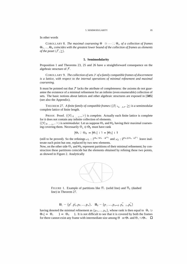
5. SEMIMODULARITY 85
In other words
COROLLARY 8. The maximal coarsening � � � � � � � � � of a collection of frames� � ��� � � ��� � coincides with the greatest lower bound of the collection of frames as elementsof the poset
� � ��� � .5. Semimodularity
Proposition 1 and Theorems 23, 25 and 26 have a straightforward consequence on thealgebraic structure of
�.
COROLLARY 9. The collection of sets�
of a family compatible frames of discernmentis a lattice, with respect to the internal operations of minimal refinement and maximalcoarsening.
It must be pointed out that�
lacks the attribute of completeness: the axioms do not guar-antee the existence of a minimal refinement for an infinite (even enumerable) collection ofsets. The basic notions about lattices and other algebraic structures are exposed in [505](see also the Appendix).
THEOREM 27. A finite family of compatible frames� � � � ( ��� � � � ��� � ��� � is a semimodular
complete lattice of finite length.
PROOF. Proof.� � � � ( ��� � � � ��� � ��� � is complete. Actually each finite lattice is complete
for it does not contain any infinite collection of elements.� � � � ( ��� � � � ��� � ��� � is semimodular. Let us suppose � � and � � having their maximal coarsen-ing covering them. Necessarily � � � � � must have rank
� � � � � � � � � � �� � � � � � � � � �
(still to be proved). So the refinings � � � ��� � � � � � ��� � and ����� ��� � � � � � ��� � leave inal-terate each point but one, replaced by two new elements.Now, on the other side � � and � � represent partitions of their minimal refinement; by con-struction these partitions coincide but the elements obtained by refining these two points,as showed in Figure 2. Analytically
FIGURE 1. Example of partitions like � � (solid line) and � � (dashedline) in Theorem 27.
� �� � � � � ��� �� ��� � ��� � � ��� � #�� �� � � � � ��� � � ��� � � � ��� � �� � � ���
� �� #having denoted the minimal refinement as
� � � ��� � � ��� � # , whose rank is then equal to� � � �� � � � � � �
� � � � � � � � � � . It is not difficult to see that it is covered by both the framesfor there cannot exist any frame with intermediate size among � � or � � and � �� � � .
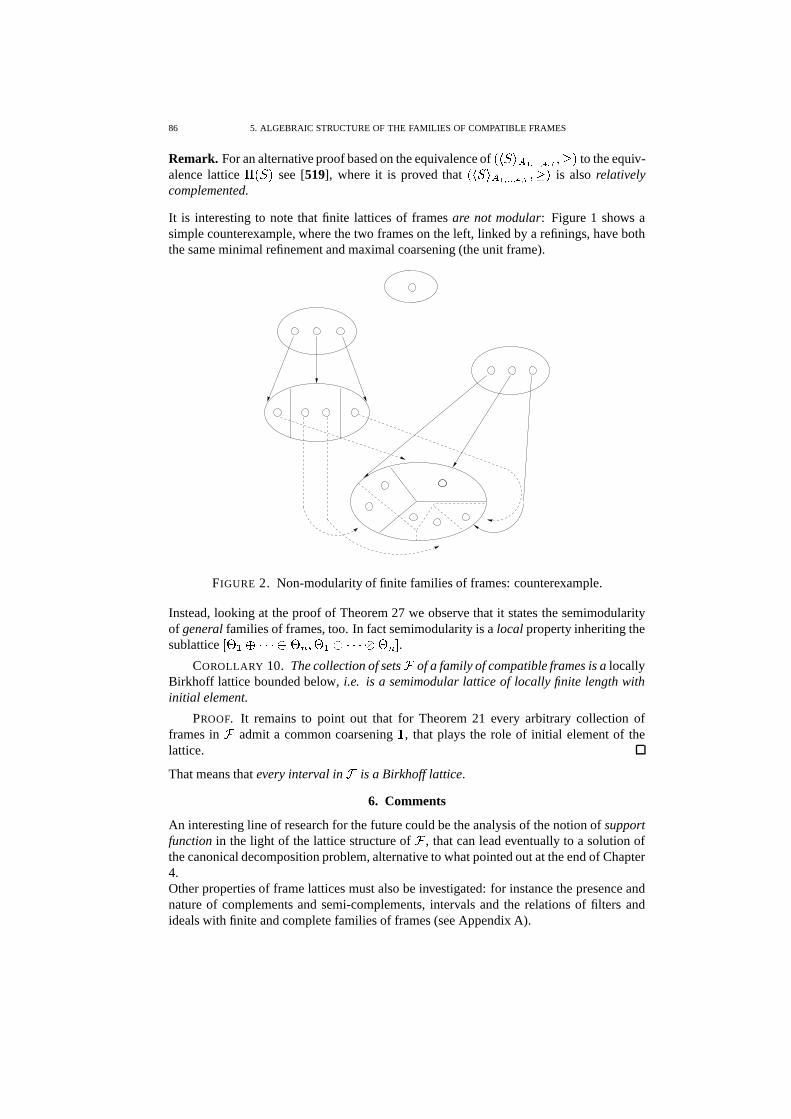
86 5. ALGEBRAIC STRUCTURE OF THE FAMILIES OF COMPATIBLE FRAMES
Remark. For an alternative proof based on the equivalence of� � � � ( ��� � � � ��� � ��� � to the equiv-
alence lattice � � � � see [519], where it is proved that� � � � ( ��� � � � ��� � ��� � is also relatively
complemented.
It is interesting to note that finite lattices of frames are not modular: Figure 1 shows asimple counterexample, where the two frames on the left, linked by a refinings, have boththe same minimal refinement and maximal coarsening (the unit frame).
FIGURE 2. Non-modularity of finite families of frames: counterexample.
Instead, looking at the proof of Theorem 27 we observe that it states the semimodularityof general families of frames, too. In fact semimodularity is a local property inheriting thesublattice � � � � � � � � � � ��� ��� � � � � � � ! .
COROLLARY 10. The collection of sets�
of a family of compatible frames is a locallyBirkhoff lattice bounded below, i.e. is a semimodular lattice of locally finite length withinitial element.
PROOF. It remains to point out that for Theorem 21 every arbitrary collection offrames in
�admit a common coarsening
�, that plays the role of initial element of the
lattice.
That means that every interval in�
is a Birkhoff lattice.
6. Comments
An interesting line of research for the future could be the analysis of the notion of supportfunction in the light of the lattice structure of
�, that can lead eventually to a solution of
the canonical decomposition problem, alternative to what pointed out at the end of Chapter4.Other properties of frame lattices must also be investigated: for instance the presence andnature of complements and semi-complements, intervals and the relations of filters andideals with finite and complete families of frames (see Appendix A).

CHAPTER 6
Independence and conflict
1. Subspace and frame lattices
We are now able to precise the analogy between the familiar notion of vector spaceand the evidential notion of frame of discernment. It is well known, in fact, that the setof the subspaces of a finite-dimensional vector space V is a lattice, too: a modular [216]lattice in particular, where � is the order relation,
the smaller upper bound, while � � ���
is the greatest lower bound.
FIGURE 1. The subspace lattice.
These similarities are summarized in the following table.
� � � �
initial element 1� $ # �
smaller upper bound � � � � � ��� � '����� � � �
greatest lower bound � � � � � � �
order relation � � � � � � � refining s.t. � ����� � � �
rank � � � � � � ' � � � � �87
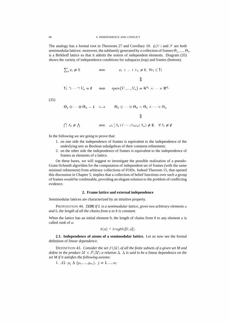
88 6. INDEPENDENCE AND CONFLICT
The analogy has a formal root in Theorems 27 and Corollary 10. � � � and�
are bothsemimodular lattices: moreover, the subfamily generated by a collection of frames � � ��� � � ��� �is a Birkhoff lattice so that it admits the notion of independent elements. Diagram (35)shows the variety of independence conditions for subspaces (top) and frames (bottom).
� � � � �� � � � � �� � � � � ��� �� � � � �
� ) ���
� � � � -� � $ � � � � ��� � � ��� � � �� -� # ����� � � � � � � ��� �
� � � � � � � � � � � � � � � � � � � � � � �� ��� � � � � � ���
� � � �� � � � � �� � � � � � � ��� � �� � �� $ � � �
� �� $
(35)
In the following we are going to prove that:
1. on one side the independence of frames is equivalent to the independence of theunderlying sets as Boolean subalgebras of their common refinement;
2. on the other side the independence of frames is equivalent to the independence offrames as elements of a lattice.
On these bases, we will suggest to investigate the possible realization of a pseudo-Gram-Schmidt algorithm for the computation of independent set of frames (with the sameminimal refinement) from arbitrary collections of FODs. Indeed Theorem 15, that openedthis discussion in Chapter 5, implies that a collection of belief functions over such a groupof frames would be combinable, providing an elegant solution to the problem of conflictingevidence.
2. Frame lattice and external independence
Semimodular lattices are characterized by an intuitive property.
PROPOSITION 44. [519] If L is a semimodular lattice, given two arbitrary elements �and � , the length of all the chains from a to b is constant.
When the lattice has an initial element 0, the length of chains from 0 to any element � iscalled rank of � :
� � � � �� �� � � � � � � � � ! ���2.1. Independence of atoms of a semimodular lattice. Let us now see the formal
definition of linear dependence.
DEFINITION 43. Consider the set� ��� � of all the finite subsets of a given set M and
define in the product� � � ��� � a relation � . � is said to be a linear dependence on the
set M if it satisfies the following axioms:
1. � � : ��� � � � ��� � � ��� 0 #�� � ��� ��� � � �!� �
2. FRAME LATTICE AND EXTERNAL INDEPENDENCE 89
2. �� : if � � � � � ��� � � ��� 0 # and � � � ��� � � � ��� � � � � � # then � � � � � ��� � � � � � # �
3. � �: if � � � � � ��� � � ��� 0 � � # but � � � � � � ��� � � ��� 0 # then � � � � � ��� � � ��� 0 ��� #��
If L is a semimodular lattice a linear dependence relation� �
can be introduced over theset � of its atoms (elements ”covering” 0) [519], see Appendix A.
DEFINITION 44. � � � � � � ��� � � � � 0 #���� � � � ��� � � � � 0 ) � if
� % � �� � � � � � 0 �(36)
It is well-known that (see [519] again)
PROPOSITION 45. If L is a semimodular lattice bounded below then (36) is a lineardependence relation, i.e. it satisfies the axioms of Definition 43.
It is easy to see that� �
generalizes the notion of independence of vectors of a linear space,for they are exactly the atoms of the lattice L(V).A finite set of atoms
� � � � � ��� � � ��� 0 # is said to be linearly independent (L.I.) if
�(����� � � � � � � #��
PROPOSITION 46. For all nonempty set of atoms of a semimodular lattice L it is pos-sible to select a maximal set of L.I. atoms and every set of L.I. atoms can be extended to amaximal one.
PROPOSITION 47. A finite set� � � ��� � � ��� 0 # of atoms is L.I. iff
� � �� � � � � � � � � � � � � � �
for� � � ��� � � �!� .
In the case of finite length we can claim that
PROPOSITION 48. If� � � ��� � � ��� 0 # are atoms of a Birkhoff lattice then
� � � �� � � � � � � ��% �
where � � � � is the rank of�
and the equality holds iff they are linearly independent.
2.2. Independence of generic elements of a semimodular lattice. The linear de-pendence relation is easily extended to generic subspaces of a vector space . Again, theindependence condition for the elements of a family of compatible frames does not regardonly the binary partitions of a finite family (which play the role of atoms in the corre-sponding lattice). If we want to establish a lattice-theoretical interpretation of the idea ofindependent frames we need to extend the above relation to generic elements of a semi-modular lattice.Let us define three different relations among generic elements of a lattice.
DEFINITION 45.� � � ��� � � ��� � # are
���� independent if
�� �% �� 46 � � � � � � � �
� � �� 46 � � � �� ��� � ���
DEFINITION 46.� � � ��� � � ��� � # are
��� � independent if
� � � � � �� � � � � � � � � � � � � � � � ��� � � �!� �
DEFINITION 47.� � � ��� � � ��� � # are
���� independent if
� � � �� � � � � � � � � � � � � � � � � � � � � � � ���
90 6. INDEPENDENCE AND CONFLICT
In [519] we can find the proof that
PROPOSITION 49. The restrictions of the above relations to the set of the atoms A ofa lattice are equivalent, namely� � � ��� � � � � � # ��� � � � � � ��� � � � � � # ��� � � � � � ��� � � � � � # ��� �when �
� ) � � � .For instance, linear independence among vectors in a vector space can be expressed in oneof the following equivalent formulations:
� � �� � � ��� � � � ��� � � � �� � ��� � � � ��� � � � �� � � � ��� � � � ��� � � � �� � ��� � � � ��� � � $ �
� � ' � � � ��� � � � ��� � � � ��� � � � �It is natural to ask what is the meaning of the above relations for arbitrary elements of alattice.
2.3. Modularity assumption and independence relations. First, let us check if re-lations
���� ,��� � and
���� are correlated and under what conditions. It is a good rule to
follow an intuition when reasoning over abstract concepts. In our case it is useful to focusover the familiar idea of vector subspace.
2.3.1. Vector subspaces and equivalence relations. It is easy to check that
THEOREM 28. In the subspace lattice��� � � ���
� .
PROOF. By hypothesis if we consider a number of subspaces � ��� � � �� -� -� �� $ � � � � ��� � � �� -� � � $ � � � � �� -� � � ��� � � ��� � � �� -� � � � � $ �
Now let us suppose that exists a subspace �� such that � ��� � ��� � � ��� � � �� � � � � � � �� ��� � ��� � � �� -� ���By hypothesis � � � ��� � � ��� � � �� � � � � � $
so that � � � � ��� � ��� � ��� � � �� -� � � � � �� $for� ) � � � � � � ��� � � �!� ! . But on the other side � � � ��� � � ��� � � �� � � � � � $ � � � � $
since� � � and we have a contradiction.
Looking at the proof of Theorem 70, page 152 in [519], rewritten as follows
PROPOSITION 50. If a finite set of atoms of a semimodular lattice bounded below is��� � then it is���
� .
we can note that it is based on the assumption that���
� is a linear independence relationamong atoms, in particular that
� ��� ���
� satisfies Axiom A3.
THEOREM 29. In the subspace lattice� �
� does not meet Axiom A3.
PROOF. If � � � ��� � � ��� � � �� 0 � �(� but �� � � ��� � � ��� � � �� 0 � then V can be de-composed as � � � ��� � � � ��� � � � ��� � � � � ��� � � � ��� � � ��� � �where � denotes the standard orthogonal decomposition and
�� ) � � ��� � � ��� � � �� 0 �
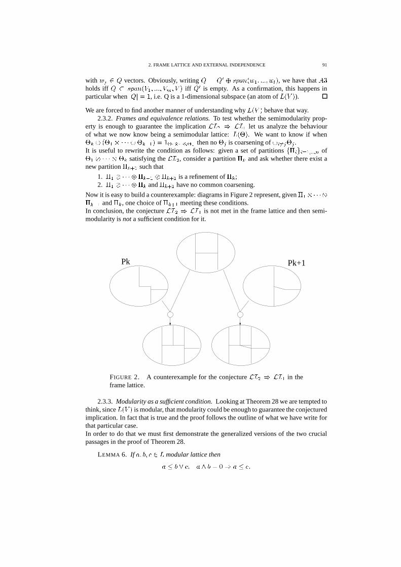
2. FRAME LATTICE AND EXTERNAL INDEPENDENCE 91
with �� ) � vectors. Obviously, writing � � � � � � � ��� � � � ��� � � ��� � � , we have that � �
holds iff � � � � ��� � � ��� � � �� 0 �� (� iff � � is empty. As a confirmation, this happens inparticular when
� � � ��� , i.e. Q is a 1-dimensional subspace (an atom of � � � ).We are forced to find another manner of understanding why � � � behave that way.
2.3.2. Frames and equivalence relations. To test whether the semimodularity prop-erty is enough to guarantee the implication
��� � � ���� let us analyze the behaviour
of what we now know being a semimodular lattice: � � � � . We want to know if when� � � � � � � � � � � � � � � � ��� � � ��� � � � � � then no � � is coarsening of �� 46 � � � .
It is useful to rewrite the condition as follows: given a set of partitions� � � # � 6 � � � � of� � � � � � � � � satisfying the
��� � , consider a partition � � and ask whether there exist anew partition ����� � such that
1. � � � � � � � ��� � � � ����� � is a refinement of � � ;2. � � � � � � � ��� and ����� � have no common coarsening.
Now it is easy to build a counterexample: diagrams in Figure 2 represent, given � � � � � � ���� � � and ��� , one choice of � ��� � meeting these conditions.In conclusion, the conjecture
��� � � ���� is not met in the frame lattice and then semi-
modularity is not a sufficient condition for it.
Pk Pk+1
FIGURE 2. A counterexample for the conjecture��� � � ���
� in theframe lattice.
2.3.3. Modularity as a sufficient condition. Looking at Theorem 28 we are tempted tothink, since � � (� is modular, that modularity could be enough to guarantee the conjecturedimplication. In fact that is true and the proof follows the outline of what we have write forthat particular case.In order to do that we must first demonstrate the generalized versions of the two crucialpassages in the proof of Theorem 28.
LEMMA 6. If � ��� � ) � modular lattice then
� % � � � � � � � � � � % "�
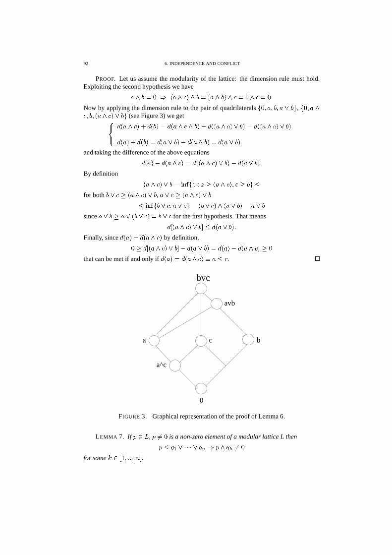
92 6. INDEPENDENCE AND CONFLICT
PROOF. Let us assume the modularity of the lattice: the dimension rule must hold.Exploiting the second hypothesis we have
� � � � � � � � � � � � � � � � �"� � � � � � ���Now by applying the dimension rule to the pair of quadrilaterals
� � � � ��� � � � �$# , � � � � � ��� � � � � � � �$# (see Figure 3) we get�� � � � � � � � � � �"� � � � � � � �"� � � � � � � � � �"� � � � � � � � � �"�
� � � � � � � �"� � � � � � �"� � � � � � �"� � � � � � �"�and taking the difference of the above equations
� � � ����� � � � � � � � � � � � � �"�*��� � � � �"���By definition � � � � � � � � ��� � � � � � � � � � � � � �$# %for both � � � � � � � � � , � � � � � � � � �
% � ��� � � � � � � # � � � � � � � � � �"� � � � �since � � �� � � � � � � � � � for the first hypothesis. That means
� � � � � � � � ! % � � � � �"���Finally, since � � � ��� � � � � � by definition,
� � � � � � � � � � ! ��� � � � �"� � � � � ����� � � � � � �that can be met if and only if � � � � � � � � � � � � % .
a c
bvc
avb
b
a^c
0
FIGURE 3. Graphical representation of the proof of Lemma 6.
LEMMA 7. If � ) � , � �� � is a non-zero element of a modular lattice L then
� % � �� � � � � � � � � � � � �� �
for some� ) � � ��� � � �!� ! .
2. FRAME LATTICE AND EXTERNAL INDEPENDENCE 93
PROOF. If the thesis was false by Lemma 6 we would have���������������� % � � � � � � � � �� % � �
� � � � � � � � � �� � �� % � �
� � � � � � � � �
with � � �� �� � � � , so that the hypothesis of Lemma 6 still holds. It is easy to see that by
applying it iteratively we would finally get
� % � � � � � � � �� � � �� ��� �
that is a clear absurdum.
Now we can easily give the general proof.
THEOREM 30. If L is a modular lattice bounded below then��� � � ���
� .
PROOF. Let assume that �������������������
� � � � �� �
� � �� � � � � �
� � � � � � � � � � � �
� � �� � � � � �
� � � � � � � � � � � �but � � � � �&% � �
� � � � � � � � �� � � � � � � � � � .
If we call
� � � �� � � � � � � � � � � � � ��� �
� � � � � � �we obtain
� �&% � � � ����� � � � � � ���By means of Lemma 6 we get
� �&% � � � ��� �� � � � � � � �
Lemma 7 now implies ��� � � � �� � for some� ) � � � � �!� ! .
On the other side it is well know that in a lattice
� � � � �� � � � � � 0 � � � � � � �
� � � � � ��� ��� � � � 'so that by negation we have
� � � � � �� � � � � � � � � � �� �
contradicting the hypothesis.
94 6. INDEPENDENCE AND CONFLICT
2.4. A new equivalent condition for modularity of Birkhoff lattices.
THEOREM 31. If L is a Birkhoff lattice then���� � ��� � .
PROOF. For L is Birkhoff (see Appendix A),
� � � � � � � �"� � � � � � �"� � � � � � �"�but � � � � �"� � � � � � � � � �"� for hypothesis so that � � � � � and the equality holds.Then
� � � �� � � � � � � � � � � � �
� � � � � � � � � � � � � � � � �� � � � � �
� � � � � � � � � � � � � ! � � � � � �� � � � � � � � � � � � � !
so that � � � � �� � � � � � � � � � � � � ! from what
� � �� � � � � � � � � � � � � � � .
We can inductively reproduce the above reasoning for� � �� � � � � � � � � � � � ��� � � �!� � � so
the thesis easily follows.
THEOREM 32. If L is a modular Birkhoff lattice then��� � � ���
� .
PROOF. By hypothesis, for all�
�� � �� 46 � � � � �
so that � � �� � � � 46 � � � � � � and being L modular, for all
�
� � � �� � � � � � � � � � � � � � � � � �� 46 � � � �
and in particular
� � � �� � � � � � � � � � � � � � � � � � � � � � � � � � � �
� � � � � � � � � � � � � � � � � � � � � � � � ��� � � � � � � � � � � � � � � � � !but by hypothesis � � � � � 46 � � � � � so that
� � � � � � � � � � � � � � � � � � � � � � � � � � � � � � � � � ! � � �
� � � �� � � � � � � � � � � � � � � � � � � � � � � � � � � � � � � � ���
By iteration the thesis follows.
As a straightforward consequence,
COROLLARY 11. if L is a modular Birkhoff lattice, then relations��� � and
���� coin-
cide.
A strongest result can be established, but we first need to prove an interesting property ofsemimodular lattices.
LEMMA 8. If L is a Birkhoff lattice, i.e. it has finite length and is semimodular, then� � � �"� � � � � � � � �
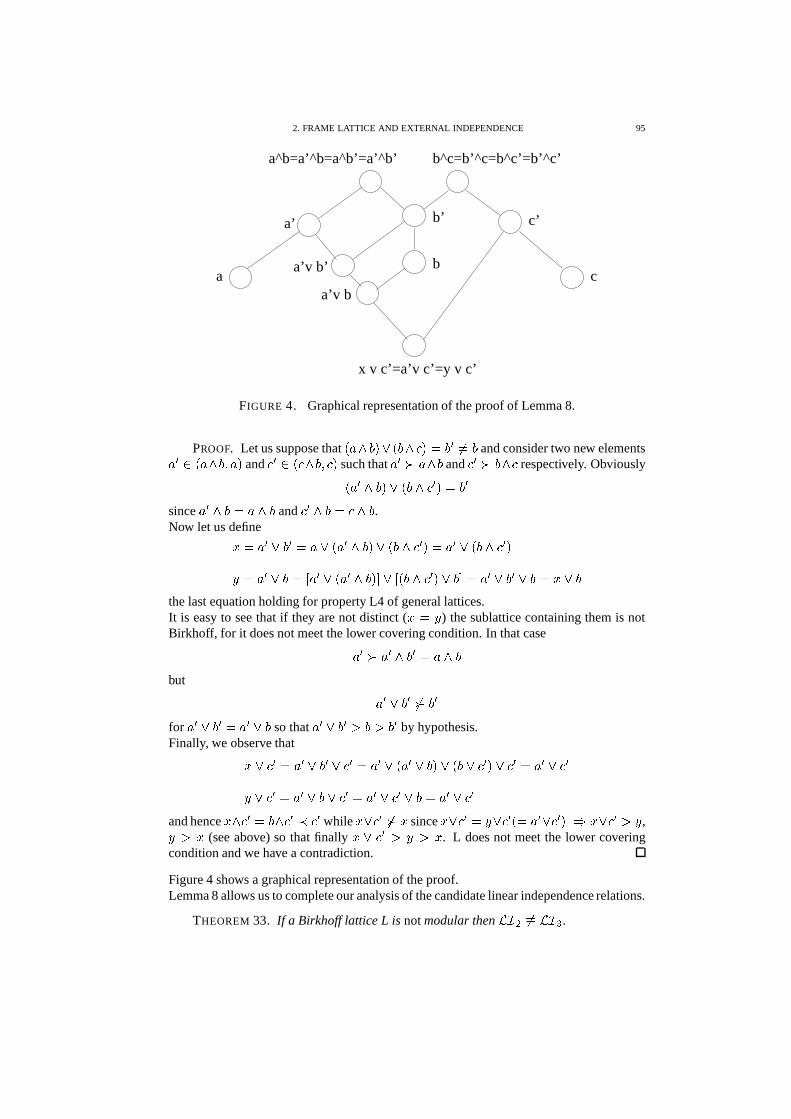
2. FRAME LATTICE AND EXTERNAL INDEPENDENCE 95
c’a’
b^c=b’^c=b^c’=b’^c’a^b=a’^b=a^b’=a’^b’
b’
ba’v b’
a’v b
x v c’=a’v c’=y v c’
ca
FIGURE 4. Graphical representation of the proof of Lemma 8.
PROOF. Let us suppose that� � � �"� � � � � � � � � �� � and consider two new elements
� � ) � � � � � � � and � ) � � � � � such that � ��� � � � and ��� � � respectively. Obviously� � � � �"� � � � � � � � � �
since � � � � � � � � and � � � � � � .Now let us define
� � � � � � � � � � � � � � �"� � � � � � � � � � � � � � � �� � � � � � � � � � � � � � � �"� ! � � � � � � � � � ! � � � � � � � � � � � �
the last equation holding for property L4 of general lattices.It is easy to see that if they are not distinct (
� � �) the sublattice containing them is not
Birkhoff, for it does not meet the lower covering condition. In that case
� � � � � � � � � � � �but
� � � � � �� � �for � � � � � � � � � � so that � � � � � � � � � � by hypothesis.Finally, we observe that
� � � � � � � � � � � � � � � � � � � �"� � � � � � � � � � � � � �� � � � � � � � � � � � � � � � � � � � � �
and hence� � � � � � ��� � while
� � � �� �since
� � � � � � � � � � � � � � � � � � � � ,� � �(see above) so that finally
� � � � � � �. L does not meet the lower covering
condition and we have a contradiction.
Figure 4 shows a graphical representation of the proof.Lemma 8 allows us to complete our analysis of the candidate linear independence relations.
THEOREM 33. If a Birkhoff lattice L is not modular then��� � �� ���
� .

96 6. INDEPENDENCE AND CONFLICT
LI1
LI2
LI3 LI2=LI3
LI1
FIGURE 5. General picture of the relations among���
� ,��� � and
����
for semimodular and modular lattices respectively.
PROOF. Since L is not modular there exist � ��� s.t. � � � � � � � �"� � � � � � �"� � � � � � �"� .Given an arbitrary element � ) � we can add � � � � to both members obtaining
� � � � � � � � � � � � �"� � � � � � �"� � � � � � �"� � � � � � �
� � � � � � � � � � � � � � �"� � � � � � �"� � � � � ��� � � �"���(37)
Now if we choose a semicomplement of � that is not a semicomplement of �� � � � � � � � � � �� �
we have
� � � � �"� � � � � � � � � � � �"� � � � � �"� � � � � � � � � � � � � � � � � �"� � � � � � �� � � � � � � � � � � � � � �"� � � � � � �� � � � � � �"� � � � � � � �"� � � � � � � � � � � � �"� � � � � � � �"� � � � � � �� � � ��� � � � � � � �"� � � � � � � � � � � � � �"� � � � � � �
so that if we call � � � � � � �"� � � � � � � � � � �"� � � we obtain � � � � �"� � � � � ��� � � � � � .Now, since � � � � for Lemma 8,
� � �"� % � � � � �"� � � � � � � � � � �"� ��� � � � � �"�*� � � � �and by substituting the last expression in Equation (37) we get
� � � � � � � � � � � � � � �"� � � � � � �"� � � � � ��� � � � � �"��� � � � � � � � � � �"���In the hypothesis that � � � �
� � � � � � � � � � �"� � � � � � ! � � � � � � �"� � � � � � �for � � � � � �"� � � (lattice property � � ). Finally � � � � � � � �"� � � � � � � � , with � � � � � .
COROLLARY 12. A Birkhoff lattice L is modular iff��� � � ���
� .
Corollary 12 states that for Birkhoff lattices��� � � ���
� is a condition equivalent tomodularity and can be used to prove it without resorting to the definition. Figure 2.4 showsa summary of the inclusion relations above proved.
2. FRAME LATTICE AND EXTERNAL INDEPENDENCE 97
2.5. A general independence relation for Birkhoff lattices. The above discussionsuggests that
���� could be the general form of the linear independence relation for semi-
modular lattices, since the structures L(V) and�
share this property.The following result confirms our conjecture.
THEOREM 34. If L is a Birkhoff lattice the equivalence relation� � � � � � � � �
defined as
� � � � � � ��� � � ��� � # � � � � � � �� � � � � � � � � � � � �
� � � � � � � � � � � � �(38)
where � ��� � ��� � � ��� � ) � and h is the rank of the elements of the lattice, is a linear depen-dence relation.
PROOF. Axiom � � : �� � � � � � ��� � � ��� � # .
� � �� � � �
� � � � � � � � � � � � �� � � � � � � � � � � � �
� � � � � � � � � � � � � �if � � �
�� �� � , i.e. �
� �� � .
Axiom � �: if � � � � � � ��� � � ��� 0 � � # but � ��� � � � ��� � � ��� 0 # then
� � � � � � ��� � � ��� 0 ��� # . If
� � � � � �� � � � � � 0 � � � � � � � �
� � � � � � 0 � � � � � � � �and
� � � � � �� � � � � � 0 � � � � � �
� � � � � � 0 � � � � � �then for the second hypothesis
� � � �� � � � � � 0 � � � � � � � � � � � � �
� � � � � � 0 � � � � � � � � � � ���for � � � � � � � �"� � � � � � �"� � � � � � �"� � � � � � �"� since L is Birkhoff,
� � � � �� � � � � � 0 � � � � � � � � �
for the first hypothesis� � � � � � �
� � � � � � 0 � � ���Axiom �� : if � � � � � � ��� � � ��� 0 # and �
� � � � � � ��� � � � � � # � � then � � � � � � ��� � � � � � # .Exploiting the first hypothesis we get, denoting
� �� � �� � � � � � � ,
� � � � � � � � � � � � � � � � � � � � � � �� � � � � � � � � � � � � � � � � � � � � � � � � � � � � � � � � � � � � � � � � � � �
so that
� � � � � � � � � � � �� ����� � � � � � � �
� � � � ���On the other side
� � � � � � � � � � � � � � � � ��� � � � � � � � � � � � � � � � � � � � � � � � � � �� � � � � � � � � � � � � � � � ��� � � � � � � � � � � � � � � � � � � � � � � � � � �
therefore by comparison one inequality must be a strict one for each line, namely
� � � � � � �� ����� � � � � �
� � � � � ��� � � � � � � � � � � � � � � � � � � � � � � �������

98 6. INDEPENDENCE AND CONFLICT
3. Equivalence of internal and external independence
At this point it is not surprising to see that��� � � �
generalizes both the linear indepen-dence of vector subspaces and the independence of frames.
PROPOSITION 51. The elements of a collection � � ��� � � ��� � of compatible frames areindependent iff the corresponding Boolean sub-algebras of their minimal refinement areindependent.
PROOF. See [439]
Remark. Independence is a local property of collections of frames.
THEOREM 35. � � ��� � � ��� � are independent as compatible frames iff they are linearindependent as elements of a Birkhoff lattice.
PROOF. Condition 4 of Theorem 15 is equivalent to � � � � � � � � � � � � � � � � � � �� � � � � � � � � where � � � � � � � � � is the rank of � as element of the lattice�
.When we note that
� � � � � � ��� � � ��� � # �
� � � � � � �� � � � � � � � � � � � �
� � � � � � � � � � � � � � � � � � � � � � � � � � � � � � � � � �and, for the lattice
�
� � � � � � ��the thesis immediately follows.
4. Conflicting evidence and pseudo Gram-Schmidt algorithm
In conclusion, we now know that:# vector subspaces of a finite-dimensional vector space and compatible families of
frames share the structure of complemented semimodular lattice ( � � (� in particu-lar is a modular lattice);# the elements of these lattices (subspaces and frames) are commutative monoids.
A vector space, indeed, is a group with respect to the operation ”+” and a frame is a Booleanalgebra, i.e. a complete distributive lattice, hence they are both commutative monoids.These remarks suggest a possible method to solve the conflict among measurement belieffunctions without resorting to the conflict graph. The well-known Gram-Schmidt orhonor-malization procedure is used to select a new set of independent vectors from an arbitraryone, resting on the independence condition and the projection of vectors onto other sub-spaces.Analogously, a pseudo Gram-Schmidt method, starting from a set of belief functions de-fined over a finite collection of frames, would detect another subset of independent framesof the same family
� � ��� � � ��� � )�� � � � � � ��� � � ��� �0 )��
� � ��� � � � �$� � � ��� � ��� � � � ���0(39)
with ' �� � in general. Once projected the � � ��� � � � �$� onto the new set of frames we wouldachieve a set of combinable belief functions � � � ��� � � � ���0 .
CHAPTER 7
Conditional belief functions and total belief theorem
1. Introduction
1.1. Data association. The data association problem is one of the more intensivelystudied computer vision applications for its importance in the implementation of automateddefense systems, and its connections to the classical field of structure from motion, whereyou want to reconstruct a rigid scene from a sequence of images.A number of feature points moving in the 3D space are followed by one or more camerasand appear in a sequence of images as unlabeled points (i.e. we do not know what are thecorrespondence between points of two consecutive frames). A common example concernsa set of markers set at fixed positions on a moving articulated body. In order to reconstructthe trajectory of the cloud of ”targets” (or of the underlying body) we need to associatefeature points belonging to pairs of consecutive images, � � and � ��� � .
The most famous approach to the data association problem (the joint probabilisticdata association filter, [14]) rests on the implementation of a number of Kalman filterseach associated to a feature point whose aim is to predict the future position of the feature,in order to produce the most probable labeling of the cloud of points in the next image.Unfortunately this method suffers a number of drawbacks: for example, when severalfeatures converge to a small region (coalescence, [43]) the algorithm cannot distinguishbetween them. Several techniques have been proposed to overcome problems like this likethe condensation algorithm [213] due to Michael Isard and Andrew Blake.
In the first part of this Chapter we prospect a solution of the model-based data asso-ciation task, where feature points represent fixed positions on an articulated body whosetopological model is known, based on the evidential reasoning. The logical informationcarried by the topological model can be expressed in term of belief functions defined overa suitable discrete space, and combined with the probabilistic information carried by thefilters usually associated to the targets in the standard JPDA approach.A tracking process resembling a filtering procedure can be set up, where the past knowl-edge represented by the current belief estimate of the model-feature associations is contin-uously refined by means of the new evidence.
1.2. Conditional functions and total belief. Unfortunately, the rigid motion con-straint derived from the topological model of the body can be expressed in a conditionalway only: in fact, to test the rigidity of the motion of two measured points at time
�, we
need to know the correct association between points of the model and measured ones attime
� � �Hence, the task of combining conditional belief functions emerges: unfortunately, as
we have seen in Chapter 2, the theory does not provide any description which could playthe role of the total probability theorem in classical Bayesian theory.In the second part of the Chapter we will give a formal description of the problem of
99
100 7. CONDITIONAL BELIEF FUNCTIONS AND TOTAL BELIEF THEOREM
combining belief functions defined over restricted subsets of a frame of discernment, con-strained to meet an a-priori condition represented by a belief function over a coarsening ofthe considered frame. The minimum-size solution is required.This problem is shown to be equivalent to building a linear system with positive solution,whose columns are associated to focal elements of the candidate total belief function. Wewill introduce a class of linear transformations on the columns of this systems and showthat the candidate solutions form the nodes of a graph whose edges are transformations ofthe above class. We will show that there is always at least one path (called optimal path)driving to a valid function whenever you choose a starting point in the graph.
2. The data association problem
The data association problem consists on, given a sequence of images� � � � � # each con-
taining a number of feature points� � � � � � # associated to points of the real space, finding the
correspondences between feature points of two consecutive images that are manifestationsof the same material point,
� � � � � � � � � � � ���The task is complicated by the fact that sometimes one or more material points are oc-cluded, so that they do not compare in the image. In other situations, false features aregenerated by defects of the vision system: eventually, the number of feature points at eachtime instant is in general different, and not all of them are images of real material points.
2.1. Joint probabilistic data association. The basis principle of the most diffusedapproach to the data association problem, the joint probabilistic data association (a widerexposition can be found in [14]) is the implementation of a number of Kalman filters. Eachof them is associated to a feature point, and produces a prediction of the future position ofthe feature in order to estimate the most probable labeling of the cloud of points in the nextimage.
Let us assume that each measurement� � � � � � at time
� � �, conditioned by the past� � � � �(� � � ! � 6 � � � � (where
�(� � � � � � � � � � # � 6 � � � 0 � is the set of measurements at time�),
has a normal distribution with mean�� � � � � � � � and variance
� � � � � � .We call validation region
� ��� ���� � � � � � � � � �� � � � � � ��� � � � � �� ��% � # the zone
out of which it is improbabile to find measurements associated to the target�
. Of courseit will be an ellipse centered in the prediction
�� � � � � �� � . If the classical linear model forthe measurements is adopted�
� � � � � � � � � � � � � � � � � � � �� � � � ��� � � � � � � � � � � � �(40)
we can distinguish among a number of different filtering approaches:# nearest neighbor: the measurement closest to the prediction in the validation region
is used to update the filter;# splitting: a number of multiple hypothesis is formulated by considering all themeasurement in the validation region;# PDA filter: for each measurement at the current time the probability of being thecorrect association is computed;# optimal Bayesian filter: the same probability is calculated for entire sequences ofmeasurements.
The basis assumption of the PDA filter is that the state of system (40) also is normallydistributed around the current prediction
�� � � � � � � � with variance��� � � � � � � .
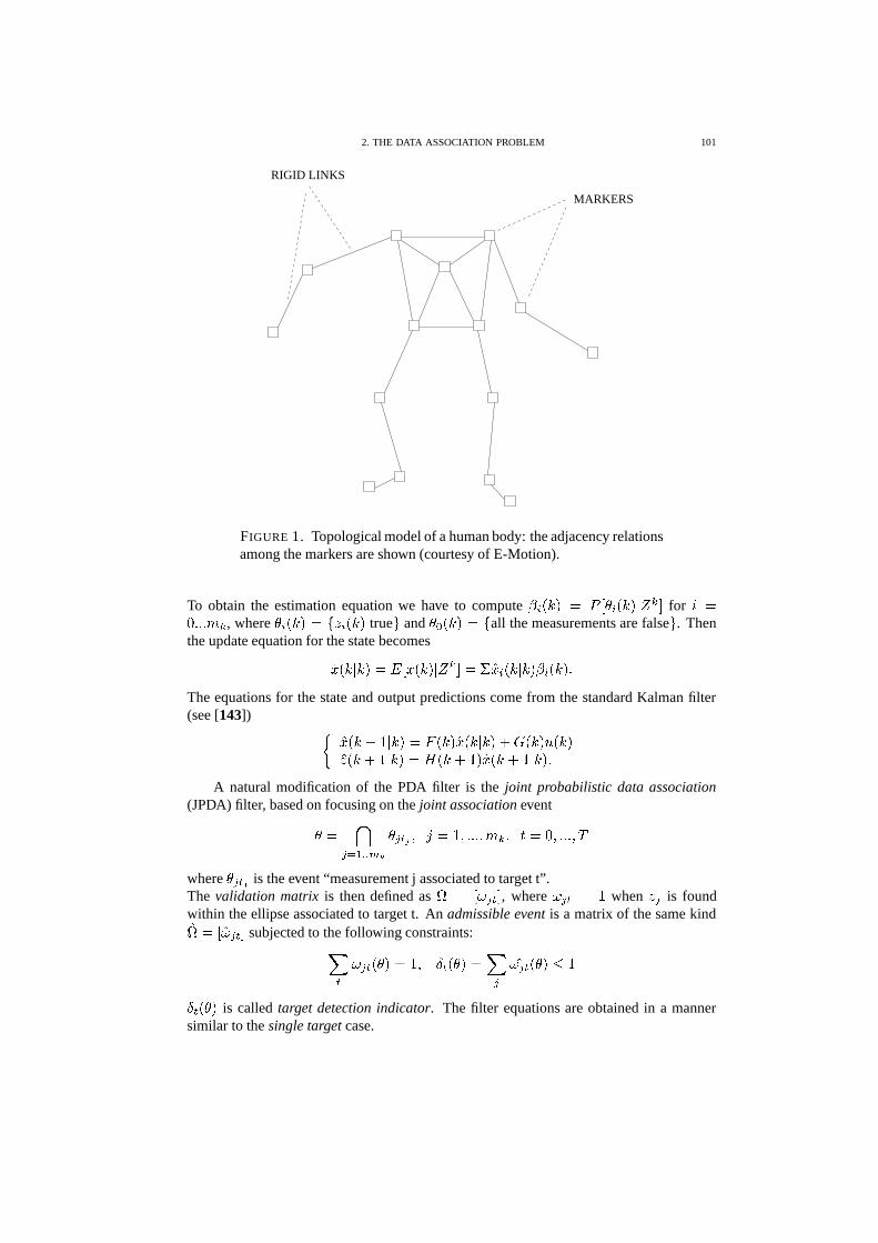
2. THE DATA ASSOCIATION PROBLEM 101
MARKERS
RIGID LINKS
FIGURE 1. Topological model of a human body: the adjacency relationsamong the markers are shown (courtesy of E-Motion).
To obtain the estimation equation we have to compute �� � � � � � � � � � � � � � � ! for
� ���� � � ' � , where � � � � � � � � � � � � true # and � 7 � � � � � all the measurements are false # . Thenthe update equation for the state becomes
�� � � � � � � � � � � � � � � � ! ��� �� � � � � � ��� � � � ���The equations for the state and output predictions come from the standard Kalman filter(see [143]) �
�� � � � � � � � � � � � � �� � � � � � � � � � � � � � ��� � � � � � � � ��� � � � � � �� � � � � � � ���
A natural modification of the PDA filter is the joint probabilistic data association(JPDA) filter, based on focusing on the joint association event
�� � �� 6 � � � 0 � �� � � � � ��� ��� � � � ' ��� � � � ��� � � � �
where � � � � is the event “measurement j associated to target t”.The validation matrix is then defined as � � � �
� � !, where �
� � � �when
� �is found
within the ellipse associated to target t. An admissible event is a matrix of the same kind�
� � � ��� � !
subjected to the following constraints:
� � � � � ��� ��� � � � � ��� � � ��� � � ����% �
� � � ��� is called target detection indicator. The filter equations are obtained in a mannersimilar to the single target case.
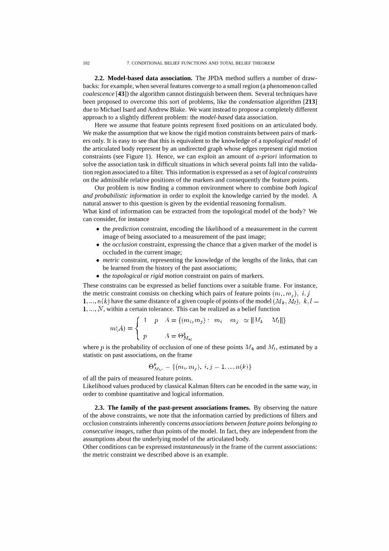
102 7. CONDITIONAL BELIEF FUNCTIONS AND TOTAL BELIEF THEOREM
2.2. Model-based data association. The JPDA method suffers a number of draw-backs: for example, when several features converge to a small region (a phenomenon calledcoalescence [43]) the algorithm cannot distinguish between them. Several techniques havebeen proposed to overcome this sort of problems, like the condensation algorithm [213]due to Michael Isard and Andrew Blake. We want instead to propose a completely differentapproach to a slightly different problem: the model-based data association.
Here we assume that feature points represent fixed positions on an articulated body.We make the assumption that we know the rigid motion constraints between pairs of mark-ers only. It is easy to see that this is equivalent to the knowledge of a topological model ofthe articulated body represent by an undirected graph whose edges represent rigid motionconstraints (see Figure 1). Hence, we can exploit an amount of a-priori information tosolve the association task in difficult situations in which several points fall into the valida-tion region associated to a filter. This information is expressed as a set of logical constraintson the admissible relative positions of the markers and consequently the feature points.
Our problem is now finding a common environment where to combine both logicaland probabilistic information in order to exploit the knowledge carried by the model. Anatural answer to this question is given by the evidential reasoning formalism.What kind of information can be extracted from the topological model of the body? Wecan consider, for instance
# the prediction constraint, encoding the likelihood of a measurement in the currentimage of being associated to a measurement of the past image;# the occlusion constraint, expressing the chance that a given marker of the model isoccluded in the current image;# metric constraint, representing the knowledge of the lengths of the links, that canbe learned from the history of the past associations;# the topological or rigid motion constraint on pairs of markers.
These constrains can be expressed as belief functions over a suitable frame. For instance,the metric constraint consists on checking which pairs of feature points
� ' � � ' � � � � � � �� ��� � � �!� � � � have the same distance of a given couple of points of the model
��� � � � � � � � � � �� ��� � � � � , within a certain tolerance. This can be realized as a belief function
' � �� ��� � � ��� � � � � ' � � ' � � � � ' � � ' � ��� � � � � � � � #� � � � �� � �
where � is the probability of occlusion of one of these points� � and
� �, estimated by a
statistic on past associations, on the frame
� �� � � � � � ' � � ' � � � � � � ��� ��� � � �!� � � � #of all the pairs of measured feature points.Likelihood values produced by classical Kalman filters can be encoded in the same way, inorder to combine quantitative and logical information.
2.3. The family of the past-present associations frames. By observing the natureof the above constraints, we note that the information carried by predictions of filters andocclusion constraints inherently concerns associations between feature points belonging toconsecutive images, rather than points of the model. In fact, they are independent from theassumptions about the underlying model of the articulated body.Other conditions can be expressed instantaneously in the frame of the current associations:the metric constraint we described above is an example.
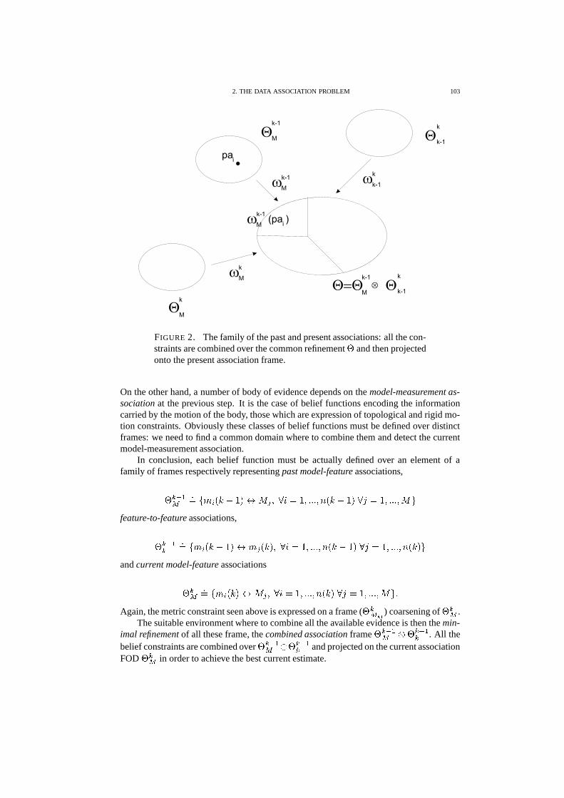
2. THE DATA ASSOCIATION PROBLEM 103
FIGURE 2. The family of the past and present associations: all the con-straints are combined over the common refinement � and then projectedonto the present association frame.
On the other hand, a number of body of evidence depends on the model-measurement as-sociation at the previous step. It is the case of belief functions encoding the informationcarried by the motion of the body, those which are expression of topological and rigid mo-tion constraints. Obviously these classes of belief functions must be defined over distinctframes: we need to find a common domain where to combine them and detect the currentmodel-measurement association.
In conclusion, each belief function must be actually defined over an element of afamily of frames respectively representing past model-feature associations,
� � � �� �� � ' � � � � � � � � � � � � � � ��� � � �!� � � � � � � ����� ��� � � � � #
feature-to-feature associations,
� � � �
� �� � ' � � � � � � � ' � � � � � � � � � ��� � � �!� � � � � � � ����� ��� � � �!� � � � #and current model-feature associations
� �� �� � ' � � � � � � � � � � ��� ��� � � �!� � � ��� � � � ��� � � � � #��Again, the metric constraint seen above is expressed on a frame ( � �� � �
) coarsening of � �� .The suitable environment where to combine all the available evidence is then the min-
imal refinement of all these frame, the combined association frame � � � �� � � � � �
� . All thebelief constraints are combined over � � � �
� � � � � �
� and projected on the current associationFOD � �� in order to achieve the best current estimate.
104 7. CONDITIONAL BELIEF FUNCTIONS AND TOTAL BELIEF THEOREM
Constraints of the third class can be expressed in a conditional way only: hence, thecomputation of a belief estimate of the current model-measurement associations impliesthe necessity of combining conditional belief functions defined over the combined associ-ation frame.In other words, the rigid motion constraint will generate an entire set of belief functions� � ��� �
��� �� 1 � � � 2 � � � � �"! over the domains
� �� �� � � � � � # � �
elements of a partition � � � � � � induced on � � � �� � � � � �
� by its coarsening � � � �� (see
Figure 2). Here � ��
is the i-th possible association at time� � � .
In order to produce a belief estimate, these family of conditional functions must bereduced to a single total belief function, that will be pooled with the other constraints.
3. Combining conditional functions
Let us now abstract from the data association problem, and state the conditions the overallfunction must obey, given a set of conditional functions � � � � � � � � � �"! over � of theelements �
�of a partition � � � � � ��� � � � � � � � # of a frame � induced by a coarsening � .
1. a-priori constraint: the restriction of the candidate total function � must be coincideto an a-priori b.f. � 7 defined on a coarsening � of the frame � ;
in the data association problem the a-priori constraint is the belief function representingthe estimate of the past association
� � ' � � � � � , defined over � � � �
� (see Figure 2again). It means that the total function must be compatible with the last available estimate.
2. Conditional constraint: the restriction � � � � of the total function � to each sub-domain must coincide with the corresponding conditional belief function � �
� � � � � � � � � ��� ��� � � � � �where
' � � �� ��� � � � � �
�� � �� �
�Exploiting the a-priori constraint we can state the following conditions over the focal ele-ments of � :
LEMMA 9. The inner reduction�� �� 1 � 2 � of every focal element of the candidate total
belief function � must be a focal element of � 7 . In other words, there must exist a focalelement ��� ) ��,
� of the a-priori function such that� 1 � 2 is a subset of � � ��� � and all the
projections � � � � , � ) ��� , have non-empty intersection with� 1 � 2 :
� � 1 � 2 ) ��, � ��� ) ��,� ��� � � � 1 � 2 ��� � � � � � � 1 � 2 � � � � �� $ ��� ) ��� �
The proof can be found in [410]. On the other hand, the conditional constraint gives thestructure the candidate f.e. must respect. If we denote with
� � 1 � 2 any candidate f.e. includedin � � ��� � ,
4. THE TOTAL BELIEF THEOREM 105
LEMMA 10. Every focal element� � 1 � 2 of the candidate total belief function � is the
union of exactly one focal element of each conditional function whose domain ��
is in-cluded in � � ��� � , where ��� is the smallest focal elements of � 7 s.t.
� � 1 � 2 ��� � ��� � i.e.� � 1 � 2 � .� ) � 1 � � 2 �
�� where
� �� ) ��, � � �PROOF. Since � � � � � � � , with ' � � �
�� ��� , for the nature of Dempster’s rule we
have necessarily � � 1 � 2 �� � � ��
for some focal element� �� of � � . Furthermore
� � 1 � 2 ��
must be non-empty, for if there
exists� � 1 � 2 � � � $
for some � � then�� �� � 1 � 2 � � ���
that is a contradiction.
This result has a fundamental consequence.
LEMMA 11. The minimum number of focal elements of the total function � belongingto � � ��� � is
� � � 6 � � � � � �� � � � � � � � � �
where � � � � +-, � and
PROOF. Called �� �
the�-th focal element of � � , the focal elements of � must satisfy for
each � � the � � � � constraints
� �
�� � �� � � ' , �� � 1 � 2 � � � '
, � �� � �' , � � �� � � � � � � � �
� � � ' , �� � 1 � 2 � �Adding the normalization constraint we have the thesis.
4. The total belief theorem
We can now formulate the analogous of the total probability theorem in the theory ofevidence.
THEOREM 36. Suppose � and � are two frames of discernment, and � � � � � ��� arefining. Let � 7 be a belief function defined over � and � � ��� � � � ��� the elements of the core+-,
� of � 7 , and there exists a collection of n belief functions � � defined over � whose cores+ �are included respectively into �
� � � � � � � # � , where � � � � � ��� � � � � � � � # is the partitionof � induced by the coarsening � .Then there exists a belief function over � ����� � � � � �"! such that:
1. � 7 is the restriction of � to � , � 7 � � � � (see Equation 7, Chapter 2);
2. the belief function obtained by combining � with
� � � ' � � � � � � � ' � �� � � � ��� � �� ��
coincide with � � for all�: � � � � � � � � � ��� ��� � � � �
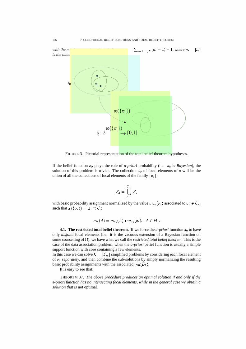
106 7. CONDITIONAL BELIEF FUNCTIONS AND TOTAL BELIEF THEOREM
with the minimum number of focal elements � � � � 6 � � � � �� � � � � � � � , where � � � � � � �
is the number of focal elements of � � .
FIGURE 3. Pictorial representation of the total belief theorem hypotheses.
If the belief function � 7 plays the role of a-priori probability (i.e. � 7 is Bayesian), thesolution of this problem is trivial. The collection
� ,of focal elements of � will be the
union of all the collections of focal elements of the family� � � # ,
��, � � � ��.� 6 �
� �with basic probability assignment normalized by the value ' , �
� ��� associated to �
� ) +-,�
such that � � � � � # � � �� � + � :' , � �� � ' , � ���� ' , �
� ��� � � ��� � �
4.1. The restricted total belief theorem. If we force the a-priori function � 7 to haveonly disjoint focal elements (i.e. it is the vacuous extension of a Bayesian function onsome coarsening of � ), we have what we call the restricted total belief theorem. This is thecase of the data association problem, when the a-priori belief function is usually a simplesupport function with core containing a few elements.In this case we can solve
� � � �-,��simplified problems by considering each focal element
of � 7 separately, and then combine the sub-solutions by simply normalizing the resultingbasic probability assignments with the associated ' 7 � ����� .
It is easy to see that:
THEOREM 37. The above procedure produces an optimal solution if and only if thea-priori function has no intersecting focal elements, while in the general case we obtain asolution that is not optimal.
5. SOLUTION SYSTEMS AND TRANSFORMABLE COLUMNS 107
PROOF. The number of constraints of the general problem (see Figure 4) is
��� � � 6 � � � � �� � � � � � � � �
on the other side, by combining the�
subproblems related to each � � ) ��,� we have
��� ��
� 6 �
�
� � 6 �
� � � � � � � � � � � 6 �
�� � � � � � � � �
where �� � � is the multiplicity of �
�, i.e. the number of focal elements ��� of � 7 such that
�� ) ��� .
Hence ��� � ��� and
��� � ��� � �� ��� � � ��� ��� � � � �
i.e the focal elements ��� are disjoint.
5. Solution systems and transformable columns
The task of finding a suitable candidate for Theorem 36 transforms into a linear algebraproblem.
5.1. Solution systems. Let � be the number of elements of a given focal element �of � 7 . The proof of Lemma 11 teaches us that a solution of the problem corresponds to alinear system with n equations and n variables
� � � � � �(41)
where each column ��
of A represents a focal element� �
of the candidate total belieffunction,
� � � ' , �� � ��� � � ' , �� � � ! and � is the number of constrains given by the N belieffunction to combine. The first � � � equations of the system have the following form
� � � � �� � � ' , �� 1 � 2 � � � '
, � �� � �' , � � �� � � � � � � �
� � � ' , �� 1 � 2 � �(where �
� �is again the
�-th focal element of � � ) or alternatively' , � � �� � � � � � �� � � ' , �� 1 � 2 ��� ' , � �
� � � � � � � �� � � ' , �� 1 � 2 � � � �(42)
while the last one is the normalization constraint
� � � �
' , �� 1 � 2 � ��� �The problem can then be reformulated in the following way: we have to choose � focalelements in the collection
� � 1 � 2 ��.� 6 �
�� � � � ) � � ��� � � �!� � ! #(43)
to form a matrix � of the linear systems 41 such that the unique solution of the system hasall positive components. For simplicity, these focal elements can be denoted by a formalvector of their components: � 1 � 2 � � �
� �� �� �� � � � � � �� ! � �
108 7. CONDITIONAL BELIEF FUNCTIONS AND TOTAL BELIEF THEOREM
5.2. Solution space and transformable columns. If we fix the instance of the prob-lem each candidate solution system is associated to a vector
��� ) � � , the solution of thecorresponding linear system:
�� � � � � � � � �� �� ��� � � � �� � �� � � �
we call�
solution space.Now, let us consider an arbitrary solution system, obtained by choosing � random
elements in the collection (43). The kind of columns that can be associated to negativecomponents of the solution is easily detectable: since the columns of the system must havepositive sum for every focal element �
� �of � � (from the constraints (42) expressed by the
rows of the system), a critical column� � must have at least one companion for every
�, i.e.
� � � � ��� � � � � � � � ��� � � � � � � � � � � � � ���In other words, a companion coincides to
� � over ��.
To this types of columns, that we call transformable, we can apply the followingtransformation:
DEFINITION 48. The class � of transformations acts on a transformable column�
ofa solution system by means of the formal sum� �� � � � � � � � � �
� � � � ��� � �(44)
where+
is an covering set of companions of�
(i.e. at least one of them cover everycomponent of
�,� + � � � ) and the selection columns � ,
� � � � � + � ��� , are used to eliminate� + � � � addenda from the formal sum and yield an admissible formal column.We call the elements of � column substitutions.
5.2.1. Effect of a transformation on a point of the solution space. A sequence of tran-sitions can then be seen as a discrete path in the solution space: the values of the solutioncomponents associated to each column vary, and in a predictable way. In fact, called � � �the solution component of the old column
�,
1. the new column� � has solution component �� � � ;
2. each companion column receives as new value � � � � � � , where � is the old one;
3. each selection column has as new value � � � � � � , where � is the old one;
4. the other columns maintain the old value for their solution components.
If we choose the column with the most negative solution component, the total effect isthat the most negative component is changed into a positive one, components associatedto selection columns are increased, while even if one or more companion columns canreceive a negative solution component, they will have an absolute value smaller then
� � �,
since � � � . Hence
PROPOSITION 52. Column transformations of the class � reduce the absolute valueof the most negative solution component, i.e. if
�is transformed into
� � by the substitution����� �� � ������ � , then� � ���� � � � ����� � �
6. SOLUTION GRAPHS 109
The length of a transition in the solution space can be easily computed from the aboveremarks, getting
���� � � 6 �
� � � � � � � � ��� � � � � � � � � � � � ��� � � ��� � � � � � ��� � � � � �
��� � � � � � � � � � � � � � ��� ��� � � � � � � � � � � � �Remark. Simple counterexamples show that the shortest path is not necessarily com-
posed by longest (greedy) steps. This means that an algorithm based on a greedy choice,or on dynamic programming cannot work, for the problem does not have the optimal sub-structure property.
The length of the longest path in the solution space, corresponding to choosing the mostnegative variable
�, and all selection columns positive, can be computed in the same way,
getting
� , � ��� , � � 6 �
��� � � � � � � � � � � � �
�� � � � � � � �&% �
�� % � �
5.3. Hint of an existence proof. Now we are able to formulate the sketch of an exis-tence proof for the restricted total belief theorem, thanks to the effects of transformationsof type � on the solution components. In fact,
1. at each transformation� � 0 � � � decreases;
2. by transforming the most negative variable we always obtain different systems, foreach transformed column receive a positive solution component, that cannot bechanged back to a negative one;
3. the number of solution systems is obviously finite, hence the procedure must ter-minate.
Now, if every column with companions on every focal element of � � could be transformableby means of a � -class transformation, the procedure could not terminate at a system withnegative variables, for they have one or more positive companions at each point.Unfortunately, there are “transformable” columns that do not admit a transformation of theclass (44), for even if they have companions on every �
�there not exists a collection of
selection columns
6. Solution graphs
If we define an adjacency relation between solution systems as� � � �
if� �
can beobtained from
� �by substituting a column by means of transformation (44) (and vice-
versa), we can rearrange the solution systems related to a problem of a given size� � � � � �
� ��� � � � � # in a solution graph.
6.1. Significant examples of solution graphs. Let us see some significant examples,and analyze their properties.
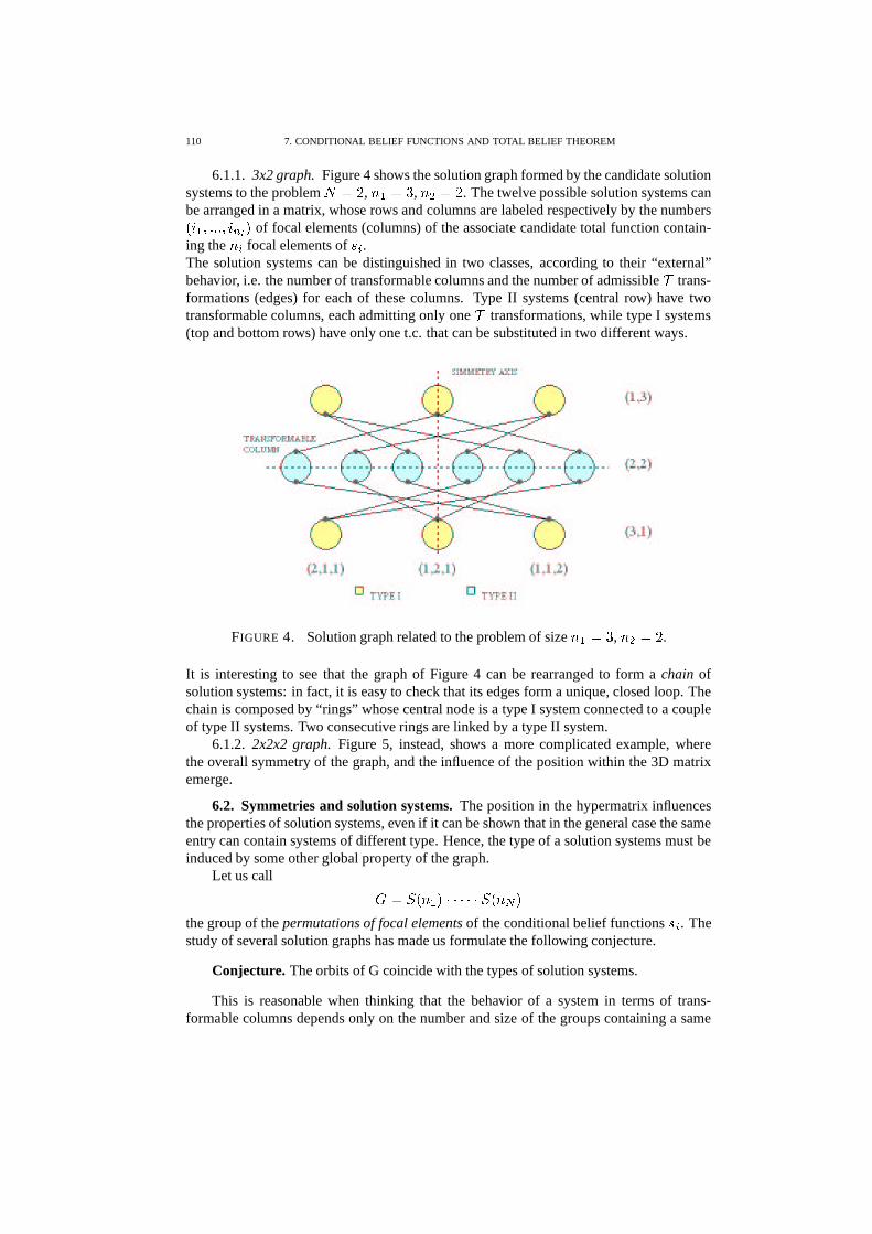
110 7. CONDITIONAL BELIEF FUNCTIONS AND TOTAL BELIEF THEOREM
6.1.1. 3x2 graph. Figure 4 shows the solution graph formed by the candidate solutionsystems to the problem � � � , � �
� �, � � � � . The twelve possible solution systems can
be arranged in a matrix, whose rows and columns are labeled respectively by the numbers� �� ��� � � � � � � of focal elements (columns) of the associate candidate total function contain-
ing the � � focal elements of � � .The solution systems can be distinguished in two classes, according to their “external”behavior, i.e. the number of transformable columns and the number of admissible � trans-formations (edges) for each of these columns. Type II systems (central row) have twotransformable columns, each admitting only one � transformations, while type I systems(top and bottom rows) have only one t.c. that can be substituted in two different ways.
FIGURE 4. Solution graph related to the problem of size � �� �
, � � � � .
It is interesting to see that the graph of Figure 4 can be rearranged to form a chain ofsolution systems: in fact, it is easy to check that its edges form a unique, closed loop. Thechain is composed by “rings” whose central node is a type I system connected to a coupleof type II systems. Two consecutive rings are linked by a type II system.
6.1.2. 2x2x2 graph. Figure 5, instead, shows a more complicated example, wherethe overall symmetry of the graph, and the influence of the position within the 3D matrixemerge.
6.2. Symmetries and solution systems. The position in the hypermatrix influencesthe properties of solution systems, even if it can be shown that in the general case the sameentry can contain systems of different type. Hence, the type of a solution systems must beinduced by some other global property of the graph.
Let us call
� � � � � � � � � � ��� � � � ��the group of the permutations of focal elements of the conditional belief functions � � . Thestudy of several solution graphs has made us formulate the following conjecture.
Conjecture. The orbits of G coincide with the types of solution systems.
This is reasonable when thinking that the behavior of a system in terms of trans-formable columns depends only on the number and size of the groups containing a same
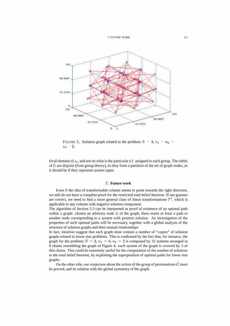
7. FUTURE WORK 111
FIGURE 5. Solution graph related to the problem � � �, � �
� � � �� � � � .
focal element of � � , and not on what is the particular e.f. assigned to each group. The orbitsof G are disjoint (from group theory), so they form a partition of the set of graph nodes, asit should be if they represent system types.
7. Future work
Even if the idea of transformable column seems to point towards the right direction,we still do not have a complete proof for the restricted total belief theorem. If our guessesare correct, we need to find a more general class of linear transformations � � , which isapplicable to any column with negative solution component.The algorithm of Section 5.3 can be interpreted as proof of existence of an optimal pathwithin a graph: chosen an arbitrary node
�of the graph, there exists at least a path to
another node corresponding to a system with positive solution. An investigation of theproperties of such optimal paths will be necessary, together with a global analysis of thestructure of solution graphs and their mutual relationships.In fact, intuition suggest that each graph must contain a number of “copies” of solutiongraphs related to lower size problems. This is confirmed by the fact that, for instance, thegraph for the problem � � � , � �
� � , � � � � is composed by 32 systems arranged in8 chains resembling the graph of Figure 4: each system of the graph is covered by 3 ofthis chains. This could be extremely useful for the computation of the number of solutionsto the total belief theorem, by exploiting the superposition of optimal paths for lower sizegraphs.
On the other side, our conjecture about the action of the group of permutations � mustbe proved, and its relation with the global symmetry of the graph.

112 7. CONDITIONAL BELIEF FUNCTIONS AND TOTAL BELIEF THEOREM
Our opinion is that the results obtained for the restricted total belief problem could beuseful to infer a line of investigation for the solution of the general issue.

Part 3
Computer vision applications

CHAPTER 8
Articulated object tracking
In this Chapter we will see another application of the evidential reasoning to a well-known computer vision problem, called articulated object tracking. We have seen that theD-S theory is a popular tool used in sensor fusion task, where data coming from severaldifferent devices must be combined in order to make decisions, or compute estimations.In a vision context, the only input device is a camera (or more then one, in stereo appli-cations). However, an image is too complex and redundant to be used directly as input toan algorithm: for each problem a number of salient information, or features is chosen andextracted from the image to be elaborated.Hence, the need of integrating the information carried by different features easily arises,specially when the observed phenomenon is particularly complex. It must be pointed outthat it is often impossible to write analytic relations between different features for they canconcern completely unrelated aspects of the images.
Object tracking is an interesting application, consisting on the reconstruction of theactual pose a moving object by processing the sequence of images taken during the move-ment. Several different approaches to this task have been developed: model-based trackingalgorithms [375] exploit optimization techniques in order to minimize a residual betweenpredicted and real measurements and achieve the set of parameters that better fits the newimage evidences. They often suffer the problematic convergence of numerical minimiza-tion algorithms and generally need to be manually initialized. Other techniques[44] aim togive qualitative descriptions of motions, in order to receive messages or recognize mean-ings; gesture recognition[498] is a typical example.All these methods are generally based on a single kind of feature which can produce misun-derstanding under particular conditions (rapid movements, for instance). Besides, model-based feature extraction can hardly carry independent evidence about the image for it isdriven by current parameter estimates.
In the following a fusion scheme based on the theory of evidence is exposed, based onthe discretization of both the parameter space � of the articulated object and the involvedfeature spaces. The properties of this evidential model are analyzed: in particular, greatattention is posed on the choice of the sample trajectory as a means for generating thediscrete version of � . Several theoretical problems we mentioned in the first part of thethesis emerge in this framework: for instance, the extraction of a pointwise estimate of thepose will be done through probabilistic approximation. The lack of a definitive algebraicsolution to the problem of conflicting measurements will force us to find an alternativemethod.
1. Evidential model
Several key ideas of the Dempster-Shafer theory are very attractive in this perspective. Itprovides a formal environment for concepts like the contemporary presence of differentkinds of representation of phenomena or different levels of precision among homogeneous
115
116 8. ARTICULATED OBJECT TRACKING
descriptions, relationships among distinct feature spaces and a measure of consistencyof the acquired data. Unfortunately, since the theory is restricted to the case of finitesets of possibilities, we are constrained to find a discrete framework in which combinatecontinuous measurements.This involves several tasks:
1. building a discrete frame of discernment approximating a continuous feature space;2. transforming the acquired feature data into belief functions over the appropriate
FOD;3. measuring their consistency level, and rejecting the discarding features;4. combining these functions in a common environment;5. extracting from the resulting b.f. an estimate of the configuration of the object.
The choice of a method for discretizing features is of course critical: naive approacheslike, for example, the regular partitioning of the measured feature range are clearly inad-equate for they introduce arbitrary subdivisions of the feature range and lose most of theinformation carried by the measurements.
1.1. Sample trajectory. In particular we need to approximate the parameter space �of the object, whose points represent internal configurations of the body. For example amanipulator with � degrees of freedom � will have in general a domain of � � as con-figuration space. Excluding pathological situations we can assume the compactness (theparameter space has no unreachable limit poses) and the connectness of � (every shapecan be assumed by an articulated object starting from any initial pose). The domain willnot be in general linearly connected: it can have cuts or holes due to position constraintsconcerning two or more parts of the object. Even a kinematic model of the object is notpowerful enough to fully describe the configuration space, for these constraints are hard toformulate and depend on the size of body.
We can overcome these obstacles by describing a sample trajectory in the parameterspace of the tracked object, i.e. collecting a significant set of configuration points
�
� �� � � � � � � � � � � ��� � � � � #for example by sampling a continuous curve
� � � .�
� must satisfy two conditions:
1. it has to be dense in � :
� � ) � � � ��� � � � � � � � � � � � ��� �2. each feature function
� �cannot have sharp variations in the � -neighborhood of a
sample point.
The first condition simply guarantees that if we choose the object estimated position in�
�we have an error smaller than � . Condition (2) ensures that each sample is a good represen-tative of its neighbors, for its feature value is similar to the others in the � -neighborhood.The following classical result demonstrates that such a trajectory exists, at least for non-pathological situations:
THEOREM 38. (Small oscillations theorem) If a function� � � � � is continuous
over a compact subset � � � � then � � � � there exists a partition � of � such that' � � � � � � ��� � � � � � � � � � ������ ��� � � � � � �
� � �� ' ��� � � ��� ) �8�
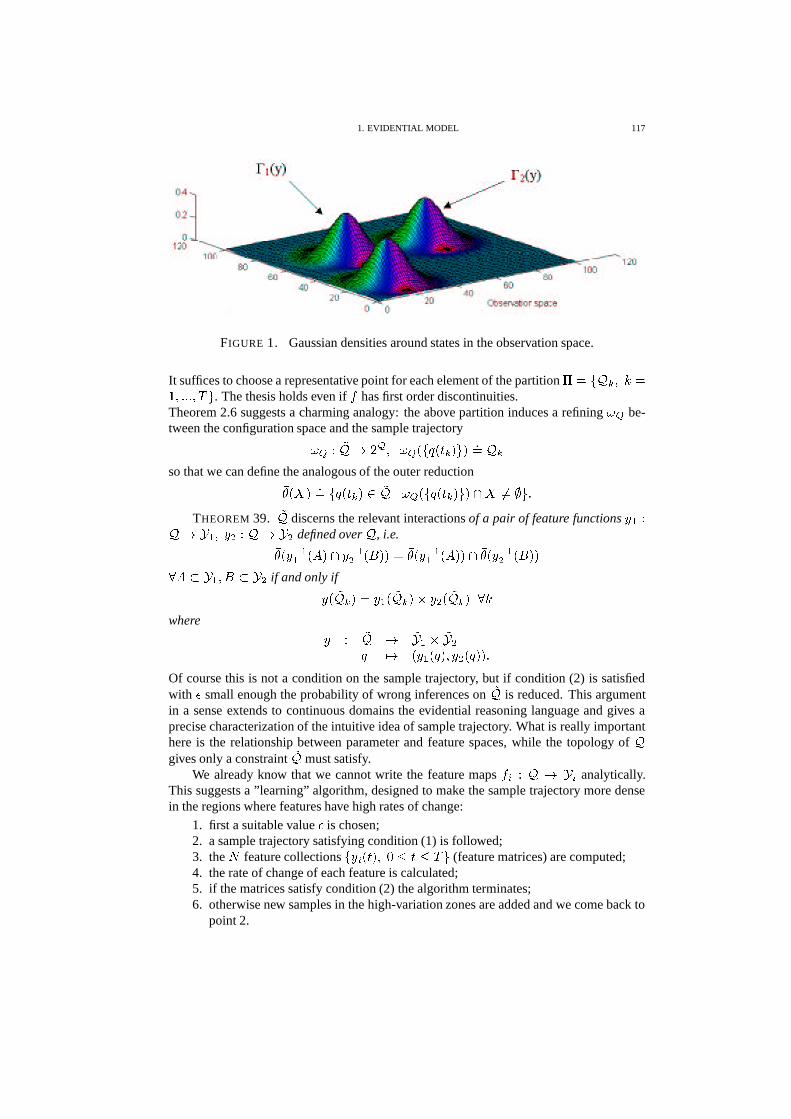
1. EVIDENTIAL MODEL 117
FIGURE 1. Gaussian densities around states in the observation space.
It suffices to choose a representative point for each element of the partition � � � � ��� � �� ��� � � � � # . The thesis holds even if
�has first order discontinuities.
Theorem 2.6 suggests a charming analogy: the above partition induces a refining ��� be-tween the configuration space and the sample trajectory
��� � �
��� � � � ��� � � � � � � � # � �� ���so that we can define the analogous of the outer reduction
�� ��� � �� � � � � � � ) �
� � ��� � � � � � � � # � � �� $ #��THEOREM 39.
�
� discerns the relevant interactions of a pair of feature functions�
� �� � �
� � � � � ��� � � defined over � , i.e.�� � � � �
�� �� � � �� ��� � � � �� � � � �
�� �� � �� � � � �� ��� � �
� � � �� � � � � � if and only if
� � �
��� � � � �� �
��� � � � � � �
��� � � �where
� � �
� � ����� �� �
� �� � ��� � � � � � � � � ���
Of course this is not a condition on the sample trajectory, but if condition (2) is satisfiedwith � small enough the probability of wrong inferences on
�
� is reduced. This argumentin a sense extends to continuous domains the evidential reasoning language and gives aprecise characterization of the intuitive idea of sample trajectory. What is really importanthere is the relationship between parameter and feature spaces, while the topology of �gives only a constraint
�
� must satisfy.We already know that we cannot write the feature maps
� � � � � � �analytically.
This suggests a ”learning” algorithm, designed to make the sample trajectory more densein the regions where features have high rates of change:
1. first a suitable value � is chosen;2. a sample trajectory satisfying condition (1) is followed;3. the � feature collections
� � � � � � � � % � % � # (feature matrices) are computed;4. the rate of change of each feature is calculated;5. if the matrices satisfy condition (2) the algorithm terminates;6. otherwise new samples in the high-variation zones are added and we come back to
point 2.
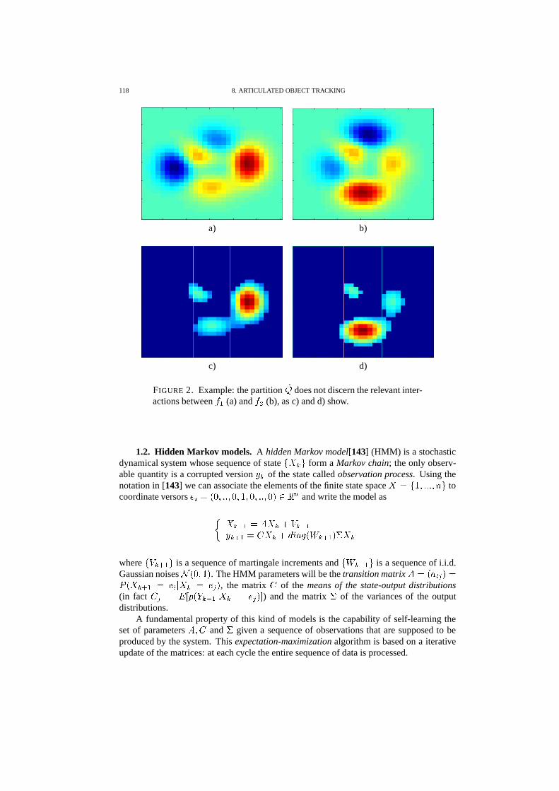
118 8. ARTICULATED OBJECT TRACKING
a) b)
c) d)
FIGURE 2. Example: the partition�
� does not discern the relevant inter-actions between
�� (a) and
� � (b), as c) and d) show.
1.2. Hidden Markov models. A hidden Markov model[143] (HMM) is a stochasticdynamical system whose sequence of state
� � ��# form a Markov chain; the only observ-able quantity is a corrupted version
� � of the state called observation process. Using thenotation in [143] we can associate the elements of the finite state space
� � � � ��� � � �!��# tocoordinate versors
� � � � � ��� � � � � � � � ��� � � ��� ) � � and write the model as�
� ��� �� � � � � ��� �
� ��� ���
� � � � � � � � ��� � � � � �
where� ��� � # is a sequence of martingale increments and
� � ��� � # is a sequence of i.i.d.Gaussian noises
��� � � � � . The HMM parameters will be the transition matrix � � � �� �� ������ ��� �
� � � � � � � � � � , the matrix
�of the means of the state-output distributions
(in fact
� � � � � � ��� ��� �� � � � � � � ! ) and the matrix
�of the variances of the output
distributions.A fundamental property of this kind of models is the capability of self-learning the
set of parameters �(��
and�
given a sequence of observations that are supposed to beproduced by the system. This expectation-maximization algorithm is based on a iterativeupdate of the matrices: at each cycle the entire sequence of data is processed.
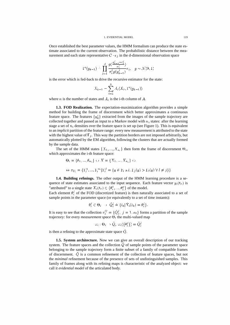
1. EVIDENTIAL MODEL 119
Once established the best parameter values, the HMM formalism can produce the state es-timate associated to the current observation. The probabilistic distance between the mea-surement and each state representative
�� � � in the d-dimensional observation space
�� � � ��� � � �� ��� 6 �
� � �� � � ��� � � � ���� � � � ��� � �
� � � ��� � � � �
is the error which is fed-back to drive the recursive estimator for the state:
�� ��� ��� � 6 �
����� � ���� � � ��� � � �
where � is the number of states and ��
is the i-th column of � .
1.3. FOD Realization. The expectation-maximization algorithm provides a simplemethod for building the frame of discernment which better approximates a continuousfeature space. The features
� � �� # extracted from the images of the sample trajectory arecollected together and passed as input to a Markov model with � � states: after the learningstage a set of � � densities over the feature space is set up (see Figure 1). This is equivalentto an implicit partition of the feature range: every new measurement is attributed to the statewith the highest value of � � . This way the partition borders are not imposed arbitrarily, butautomatically plotted by the EM algorithm, following the clusters that are actually formedby the sample data.
The set of the HMM states� �
� ��� � � � � � # then form the frame of discernment � � ,which approximates the i-th feature space:
� � � � � � ��� � � �!�"� # � � � � �� ��� � � � � � # �
� ��� � � � �� ��� � � � � � � � ��� � � � ) �
� ��� � � � � � � � � � � � � � � � �� � #�#1.4. Building refinings. The other output of the HMM learning procedure is a se-
quence of state estimates associated to the input sequence. Each feature vector� � � � � � is
”attributed” to a single state�� � � � � � ) � � �� ��� � � �!� �� # of the model.
Each element �� �
of the FOD (discretized feature) is then naturally associated to a set ofsample points in the parameter space (or equivalently to a set of time instants):
�� � ) � � � ��
� � �� � � � � �� � � � � � � �� � #��
It is easy to see that the collection� �� � � ��
� � � � � � � � � � # forms a partition of the sampletrajectory: for every measurement space � � the multi-valued map
��� � � � �� � � � � � �
� � # � � ��� �
is then a refining to the approximate state space�� .
1.5. System architecture. Now we can give an overall description of our trackingsystem. The feature spaces and the collection
�� of sample points of the parameter spacebelonging to the sample trajectory form a finite subset of a family of compatible framesof discernment.
�� is a common refinement of the collection of feature spaces, but notthe minimal refinement because of the presence of sets of undistinguished samples. Thisfamily of frames along with its refining maps is characteristic of the analyzed object: wecall it evidential model of the articulated body.
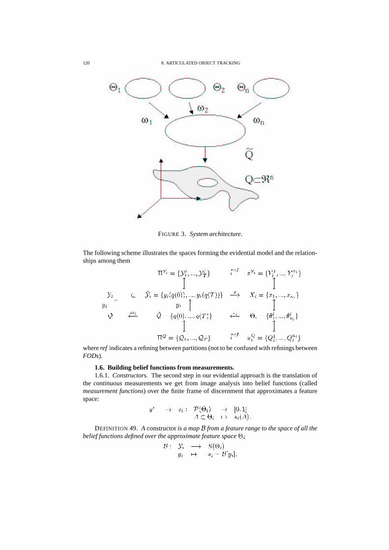
120 8. ARTICULATED OBJECT TRACKING
FIGURE 3. System architecture.
The following scheme illustrates the spaces forming the evidential model and the relation-ships among them
�� � � � �
� ��� � � � � �� # � � �� � � � � � � �� ��� � � � � � � #� ��
� ��
� � � �� � � � � � � � � ��� � ��� � � � � � � � � �� � # ��� � � � � ���� ��� � � � � � #
� � � �� � � � �� � ��
� ���� � �
� � � � � ��� ��� � � � � � �� # � � � � � � � � �� ��� � � �!� �� #� ��
� ��
� � � � � � ��� � � � � � # � � �� � � �� � � � �� ��� � � � � � � #where ref indicates a refining between partitions (not to be confused with refinings betweenFODs).
1.6. Building belief functions from measurements.1.6.1. Constructors. The second step in our evidential approach is the translation of
the continuous measurements we get from image analysis into belief functions (calledmeasurement functions) over the finite frame of discernment that approximates a featurespace:
�� � � � � � � � � � � � � � � �"!
� � � � �� � � � ����DEFINITION 49. A constructor is a map � from a feature range to the space of all the
belief functions defined over the approximate feature space � ���� � � � � � � � � �� � �� � � � � � �
� ! �
1. EVIDENTIAL MODEL 121
Constructors allow us to associate a set of measurement belief function to each configura-tion �
) � :
�� �� � � � �� � � � � � �
� �� � � � � � �� � � � � �The task of translating a single real number into a complex description like a belief functioncan simplified by decomposing the process in two steps. In the first one a set of likelihoods� � � � � �
� � �� � � � � � � � � � # � 6 � � � � � (45)
is produced. In fact, we have seen how to train a HMM and use it to make an implicitdiscretization of a feature space �
�. Given a feature vector
� � at its input, it produces asoutput the set of likelihoods
� � � � � � � # of this measurement with respect to each of the nstates of the model.
Several possible techniques of construction � � of a belief function from a set of likeli-hoods are available.
1.6.2. Bayesian constructor. The Bayesian constructor simply assigns to each ele-ment of the FOD the normalized value of the likelihood associated to the correspondentstate of the HMM:
' , � � � � # � � � � � � � � � � �� � � 6 � � � � � � � � � � �1.6.3. Discounting. Unfortunately, following Shafer[410] a Bayesian belief function
seems not to be adequate to encode an actual, finite amount of evidence: it is not a supportfunction. This obstacle can be easily overcome by applying the discounting technique:
DEFINITION 50. The discounted version of a belief function s is another b.f. � � suchthat � ' ,�� � � � � � � �' ,�� � �� � ' , � �� � � � � �.
THEOREM 40. The discounted version of a Bayesian belief function is a support func-tion.
In this context the quantity � represents the inherent uncertainty of a measurement. Itsintroduction can be useful, since discounting a function has also interesting practical ad-vantages. It can be proved that it reduces the influence of divergent functions in the com-bination process, increasing the robustness of the estimation.
1.6.4. Shafer’s constructor. A third approach comes out imposing these two condi-tions to the belief function encoding the probabilistic information:
1. it has to preserve the relative likelihood values;2. it must belong to the class of consonant b.f.
Shafer has proved that there is exactly one belief function satisfying these hypothesis. If� � � � � � # are the likelihood values associated to an observation�
then this unique b.f. isgiven by
��� �� ��� � ����� ��� �( � � � � �
����� ��� � � � � � � �
122 8. ARTICULATED OBJECT TRACKING
The assumption of consonance ensures that a set of discretized measurements receives ahigh degree of support only if it includes a large number of elements � with high likelihood.
1.7. Projections. It is interesting to analyze the maps between distinct feature spacesof the evidential model.
1.7.1. Belief projections. In our framework the evidence carried by a measured fea-ture determines an effect over the entire family of feature spaces; every belief functiongenerates a collection of ”sister” functions over the other FODs. We call them the projec-tions of the measurement function onto the other spaces of the family.
THEOREM 41. The projection of a belief function � � defined over a FOD � � ontoanother discrete feature space � � has the following expression:� �
� � � ! ��� � � � � � � �"! �� �� � � ! � �� � � � � � � � � � �
while its basic probability assignment can be computed from ' � in the following way:� �� ' � ! � �� � � ��� ��� � � � � ��� � � � �
' � ��� ���
PROOF. The vacuous extension ��� of a belief function � � ��� � � � � �"! to a refinement� , � � ��� � � � , is given by the condition ' � �� � ' � � � � �� � � ' � � � , or ([410],Theorem 7.4) ��� � � � � . Trivially, the projection
���� � � ! of a b.f. � � � ��� � � � � �"! over
another discrete feature space � � is the restriction to � � of the vacuous extension of � � to�
� , so that � �� � � ! � ���� � � � � � � � � � � � � �
On the other hand we have� �� ' � ! � �� � �
� �
��� � ��� � �
' �� � � � �
for ' �� � � � �� � iff
�is the extension of a focal element of � �
� � � � ��� � � � � ��� � � � �
' �� � � � ��� � � � � ��� ��� � � � � ��� � � � �
' � ��� ���
As a simple consequence the set of the focal elements of�-�� � � ! is
��� ��� , �� � � � � � � � � � �� � � � � ��� � � � �*) ��, #(46)
with core+�� ��� , �� � �� � � � � � +-, � � .
1.7.2. General properties. Let us see some properties of the belief projections.
THEOREM 42. If two frames are independent then the projection of a belief functionfrom one of them onto the other one is trivial:��� � �� � � � � �
� ' � ! � �� ���
for � � � �� otherwise
1. EVIDENTIAL MODEL 123
PROOF. If � � and � � are independent then�� � � � � ��� � � � � � ) � � � � � � � � # � � � ��� � �� $ # � � �
from what follows� �� ' � ! � �� � � � � � �� � � �
' � ��� � �� � � ) � ' � ��� � ��� for � � � �
� otherwise
THEOREM 43. A belief function � � , defined over � � , and its projection onto � � � � � � � !are consistent.
PROOF. � �� � � ! ��� � � � � � � � � � � ��� � � �
thus if �� ��� � � � � � �� we have
� � � � � ��� � � � � � � � � � �� � � � � � �� � � ! ��� � � � � � ����
Theorems 42 and 43 confirm that the evidential model satisfies two intuitive requests:consistency is a necessary condition for two belief functions to be joined by a projection,and independent measurements do not interact the one with the other.
1.7.3. Invariance of classes of belief functions. We can ask ourselves how the pro-jection operator transforms a measurement function of a given class, and if the resultingdescription can still represent a measured feature in the goal frame.Let us consider the behaviour of projections of Bayesian and consonant belief functions.
THEOREM 44. The projection of a Bayesian belief function can have intersecting fo-cal elements � it is not in general the vacuous extension of a Bayesian function.
PROOF. Remembering Equation (46),�� � � � � ��� � � � �� � � � � ����� � � � � � ) � � � � � � � � # � � � ��� � � �� $ # � � ) � � � � � � � � # � � � ����� � �� $ # � � � ) � � � � � � � � # � � � ����� � �� $ �
� �� � � � # � � � ��� � � �� $ #��
Of course even if the images of the focal elements of � � are disjoint (for � � is Bayesian)�� ��� � � � � ����� � � $ � � �� � , the last quantity is not guaranteed to be vacuous.
THEOREM 45. The projection ��� of a consonant belief function � is still consonant,but it has not in general the same number of focal elements.
PROOF. Let us call�
� � � � � � ���the nested focal elements of � . Obviously � � will
have as focal elements �� � �
� � ��� � � � � � � ��� � . They are all distinct subsets of�
� for � is arefining. They are also nested, so that � � is still a consonant b.f. over
�
� .Now the focal elements of
���� � � ! are all the restrictions of the subsets �
� � � � � :�� � � � � � � � � � � � � � � � � � � # � � � � � ��� �� $ #��
Since they are nested, if �� � � � # � � � � � ��� �� $
then �� � � � # � � � � � � � �� $ � � � � so that
�� � � � � � � � � � � �� � � � � � � � � � � � � �
124 8. ARTICULATED OBJECT TRACKING
i.e.� �� � � ! is consonant.
Finally it is not true in general that � � ) � � s.t. � ) �� � � � � � � � � � and � �) �� � � � � � � ��� � (it iseasy to find a counterexample). Hence in the chain
�� � � � � � �� � � � � � � � �� � � � � � ��� � �
there can be some equalities.
Theorems 44 and 45 show that among the three types of measurement functions we intro-duced above, the class of consonant belief functions is invariant under projection: hencethey can be considered the most suitable representation of feature measurements.
1.7.4. Pointwise projections. One could imagine to reverse the b.f. construction pro-cedure to extract a pointwise feature value from the belief projection: this first implies thecomputation of the likelihoods of the elements of the goal frame. The math is immediatefor consonant measurement functions, whose structure is preserved under projection. If wecall ' � ��� � � � ' � the b.p.a.’s of the nested focal elements
� � of� �� � � ! we have
� � ��� ��������� � � ' �
� ' � � � ) ��
� � � ' � � ' � � � � � ) � � � � ) � �� � �
� � ' � � � ) � � ��� ) � �� � �
� � �) +�� ��� , �For Bayesian measurement functions we can simply calculate the relative plausibilities ofthe singletons in the goal frame:
� � ��� � � � � � � ��� , �� � � � # � �� � � � � � � �� � � ! � � � � � � # � � �
again you can note the presence of a scale factor�
.After that it is necessary to detect the feature value associated to these likelihoods,
given the established implicit partition of the feature space (each region of the partition cor-responds to an element of the FOD � � ). The set of relative likelihoods
� � � � � � # � 6 � � � � � � ofthe singletons specifies a set of � � ellipsoids � � � � � � � � � � ��� � � � � ��� � � � � � associatedto each HMM state in the feature space
� �. Obviously their intersection is not guaran-
teed to be non-empty. This meets our statement that in general there is no correspondencebetween different feature measurements extracted from the same image.
2. Conflict analysis
2.1. Conflict graph and sets of compatible features. Once the measurement func-tions are projected onto to approximate state space the must be combined using Dempster’srule in order to fuse the information they carry.Unfortunately, as we have learned in Chapter 5, Theorem 15 shows that the combination isguarantee only for trivially interacting feature spaces. At each time instant any arbitraryset of measurement functions is characterized by a different level of conflict (see Defini-tion 7) in the range � � � � � !
.� � �
� means that the correspondent belief functions donot have orthogonal sum. We then need a method for detecting the most coherent groupsof b.f. and choosing one of them in order to calculate the current estimate for the objectconfiguration.
A fundamental property of the level of conflict (see Chapter 2) is:
THEOREM 46.� � � � ��� � � � �$��� � � � � � � � ��� � � � �$� � � � � � � � � � � � �$� ��� � � � �$��� � ���
2. CONFLICT ANALYSIS 125
Hence, if� , , � � � � then
� , , � , � � � � � � � , i.e. if a pair of functions is notcombinabile then all the sets of functions including this pair cannot produce any orthogonalsum. This suggests a bottom-up technique:
1. first the level of conflict is computed for every pair of measurement functions� � � � � � � � � � ����� � � � ;2. then a conflict graph is built in the following way: once decided a suitable threshold
level for the conflict, every node of the graph will represent a feature function whenedges between them will indicate a weight of conflict below the threshold;
3. recursively the subsets of combinabile b.f. with size d+1 are computed from thosewith size d by checking if the addition of any other node to the set generates acompletely connected subgraph.
This produces a number of subsets of b.f. over�� that can be chosen to produce our epis-
temic estimate.
2.2. Feature group choice criteria. We can distinguish at least three different meth-ods for choosing the “right” set of features:
1. largest subset: the group of features with the biggest size is selected;2. lowest conflict: we choose the subset with the lowest level of conflict and size over
a certain threshold;3. splitting: all the alternative estimates generated by the groups that are biggest
enough are calculated.
It should be noted that during the normal evolution of the system there is only one largeset of coherent features, even if one or two measurements can deviate from the consensus.The presence of several candidate groups with similar size reveals a pathological situation.The above feature selection methods can be tested by taking in account the associatedestimate errors. Adopting the splitting strategy we can detect in the same way the mostreliable set of features and give it a larger weight in the combination process.
2.3. Learning the conflict threshold. One may think that arbitrary choices of theconflict threshold can perhaps produce any desired estimated value. On the other hand,there is no theoretical argument supporting a precise assignment for it.An interesting approach leaves this choice to a learning procedure:
# after the implementation of the family of FODs (feature spaces, approximate pa-rameter space, refinings and projections) a new trajectory is followed;# at each time instant the measurement functions are combined (setting
�= 0 and
summing all the compatible b.f.) and the estimates are produced;# the estimate sequence is compared with the actual parameter sequence: the desiredthreshold value is obtained by taking the mean value of the sequence of w.o.c.’sweighted by the estimation errors
� � � �� � .The resulting conflict threshold will then be
�� � � � 637
� � 1 , � � � � , � 2 � � � � � � � ��� �� � � � � �Remark. As we have mentioned in Chapter 6, the conflict graph method is compu-
tationally expensive, and seems to be somehow unsatisfactory. The algebraic approachbased on the construction of a new set of measurement functions defined over independentfeature spaces we suggested at the end of Chapter 6 will be certainly the definitive solution,given both its formal elegance and greater efficiency.
126 8. ARTICULATED OBJECT TRACKING
3. Pointwise estimation
Once projected our epistemic estimate onto a suitable class, we can extract a pointwiseestimate of the object configuration by exploiting the particular form of the resulting belieffunction.
3.1. Convex parameter spaces. In the simplest case the parameter space � is con-vex. In this situation the Bayesian approximation we discussed in Chapter 4, given by thenormalized plausibility of singletons
' � � � � # � � � � , � � � # �� ��� � � � , � � � # �where
� � , � � � # � ���� � � � ��� � � # � �admits a natural representative which is a convex combination of elements in
�
� .Namely,
�� � � � �
�� � , � � � � � � ���Remark. This mechanism clearly assumes a linearly-connected parameter space (as in
the example we will see in Section 5). In more complex situations like high-dimensionalnon-linearly connected parameter spaces we must ensure that the estimate belongs to �(remember that its analytic expression is unknown).
4. Algorithms
We can finally summarize our object tracking algorithms.
4.1. Training. In the training phase the evidential model of the object is built. Thetopology of the sample trajectory is iteratively modified by increasing the number of sam-ples belonging to regions with high rate of change: this procedure has been fully describedin Section 3.2. Once the best trajectory is achieved we:
1. calculate the final feature matrices;2. process every feature matrix by a HMM obtaining:
(a) the model of the correspondent FOD � � ;(b) the refinings �
�between each FOD and the approximate parameter space
�� .
4.2. Tuning. The evidential model produced by the training algorithm still dependson a number of parameters, i.e. the dimensions
� � � � � � � � � ��# of the approximate featurespaces and the conflict threshold.The adequate number of state for a feature space can be calculated by analyzing the clus-ters the sample data form, or alternatively learned from the measured estimation error as� � increases. Even if this is formally a multi-variable optimization problem, it seems rea-sonable to calculate each single cardinality
�� � separately for they represent an inherentproperty of each feature. The level of conflict is instead estimated by means of the learningprocedure exposed in Section 4.3.

5. EXPERIMENTS 127
4.3. Tracking. Given the evidential model of the moving body, tracking an arbitrarymotion reduces to the following steps: for each time instant
�
1. the � feature vectors are calculated from the acquired image;2. each feature vector
� �is processed by the correspondent HMM
� �, producing a set
of likelihood values� �� � # ;
3. a measurement belief function � � is built from these likelihoods;4. all the measurement functions
� � � # are projected onto the discrete parameter space�� ;
5. the most coherent set of features is detected by analyzing their conflict graph, andtheir orthogonal sum (estimate function) is calculated;
6. the pointwise estimate of the object configuration is obtained through Bayesianapproximation.
Remark. It would be interesting to compute also the projections of every single mea-surement function onto the other feature FODs, and use the technique exposed in Section5 to produce � � � pointwise projected features. This way we would have for each featurea set of � � � trajectories
� �� �� # we could compare to the measured one and study theirconsistency during the tracking process.
5. Experiments
Let us see the experimental behaviour of our information integration framework in a simplesituation.
5.1. Equipment. The articulated object we have chosen is the 2 d.o.f. planar robotPantoMouse built by the Industrial Electronics group of our department. Its end-effectoris a little metallic cylinder which can move inside a
� � � � � mm area. We acquired gray-level images of
� � � � � � � pixels with a Sony XC-75 CCD camera controlled by a NationalInstruments NI-IMAQ frame grabber.As it can be seen from Figure 3a we have taken pictures of the end-effector rectangularworkspace only. The sample trajectory and a number of other robot motion were first ac-quired in batch mode by using the NI-IMAQ library of image processing routines attachedto the Labview graphical programming language, while the training and tracking routineswere developed in Matlab.
5.2. Features. To represent the images we have chosen an interesting topology-basedkind of feature called size functions which has been introduced by P. Frosini for the robustrepresentation of contours (see Figure 13.6).First ([159], [498]) we extract the silhouette of the moving body and compute two differentkind of measurement functions, called ”distance from a point” and ”distance from a line”.They are obtained by projecting the contour over a sheaf of lines passing through its centerand over spheres centered on a mesh of points respectively.
DEFINITION 51. Given a continuous function � � � � � the correspondent sizefunction
���is a map from � � � to
�which, for each pair
� � � � � ) � � � gives thenumber of connected components of the sub-domain � �
���� � ) � ��� � � � % � # that donot have an empty intersection with �9� �� � � ) � ��� � � ��% � # .By applying this technique to the above families of measurement functions we get a set of”size function tables” whose mean values collected together finally give the feature vector.As a test for our feature combination method we consider each single component of thevector as a distinct feature and build a separate FOD for it. This allows us to choose a
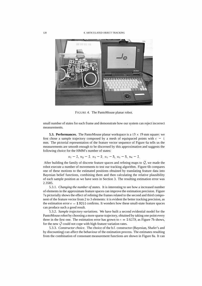
128 8. ARTICULATED OBJECT TRACKING
FIGURE 4. The PantoMouse planar robot.
small number of states for each frame and demonstrate how our system can reject incorrectmeasurements.
5.3. Performances. The PantoMouse planar workspace is a� � � � � mm square: we
first chose a sample trajectory composed by a mesh of equispaced points with � � �
mm. The pictorial representation of the feature vector sequence of Figure 6a tells us themeasurements are smooth enough to be discerned by this approximation and suggests thefollowing choice for the HMM’s number of states:
� �� � � � � � � ��� � � � ��� � � � � � � � � � � � � � �
After building the family of discrete feature spaces and refining maps to�
� , we made therobot execute a number of movements to test our tracking algorithm. Figure 6b comparesone of these motions to the estimated positions obtained by translating feature data intoBayesian belief functions, combining them and then calculating the relative plausibilityof each sample position as we have seen in Section 3. The resulting estimation error was2.3585.
5.3.1. Changing the number of states. It is interesting to see how a increased numberof elements in the approximate feature spaces can improve the estimation precision. Figure7a pictorially shows the effect of refining the frames related to the second and third compo-nent of the feature vector from 2 to 3 elements: it is evident the better tracking precision, asthe estimation error �� ��� � ��� � � confirms. It wonders how these small-state feature spacescan produce such a good result.
5.3.2. Sample trajectory variations. We have built a second evidential model for thePantoMouse robot by choosing a more sparse trajectory, obtained by taking one point everythree in the first one. The estimation error has grown to �� � � � � � ��� , as Figure 7b shows,for the new
�
� could not cope with high feature variation rates.5.3.3. Constructor choice. The choice of the b.f. constructor (Bayesian, Shafer’s and
by discounting) can affect the behaviour of the estimation process. The estimates resultingfrom the combination of consonant measurement functions are shown in Figure 8a. It can
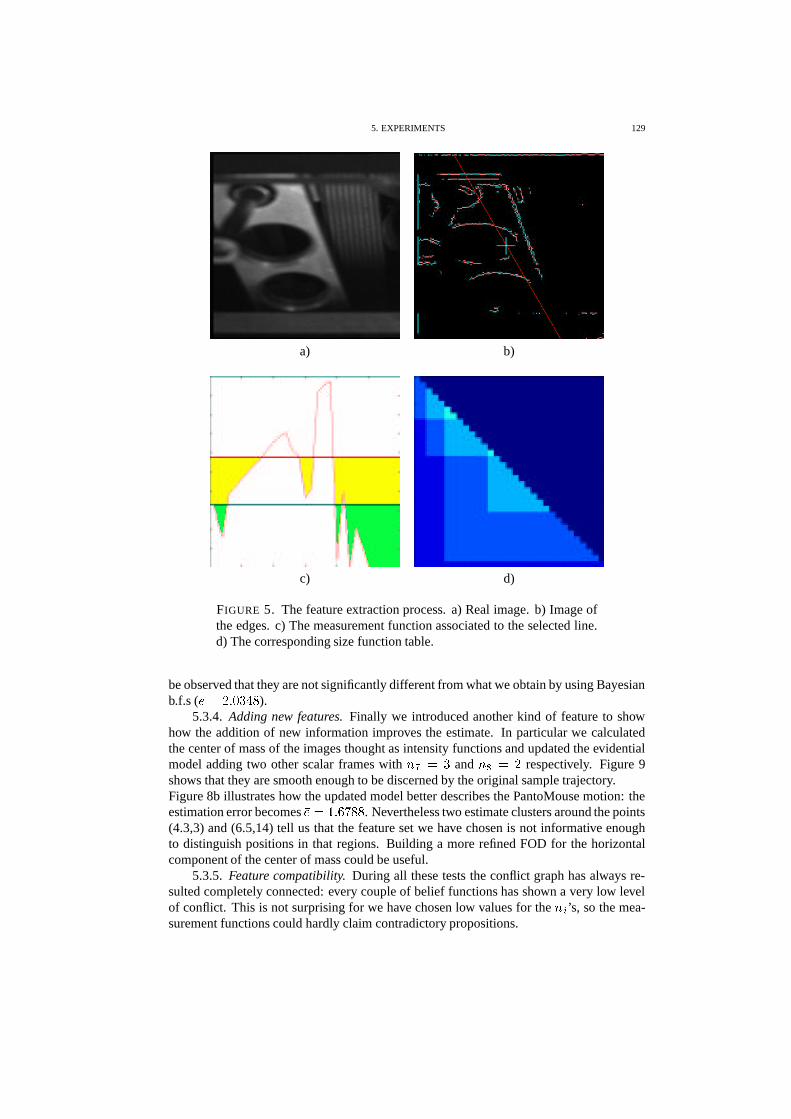
5. EXPERIMENTS 129
a) b)
c) d)
FIGURE 5. The feature extraction process. a) Real image. b) Image ofthe edges. c) The measurement function associated to the selected line.d) The corresponding size function table.
be observed that they are not significantly different from what we obtain by using Bayesianb.f.s ( �� � � � � � � ).
5.3.4. Adding new features. Finally we introduced another kind of feature to showhow the addition of new information improves the estimate. In particular we calculatedthe center of mass of the images thought as intensity functions and updated the evidentialmodel adding two other scalar frames with � � � �
and ��� � � respectively. Figure 9shows that they are smooth enough to be discerned by the original sample trajectory.Figure 8b illustrates how the updated model better describes the PantoMouse motion: theestimation error becomes �� � � � � � . Nevertheless two estimate clusters around the points(4.3,3) and (6.5,14) tell us that the feature set we have chosen is not informative enoughto distinguish positions in that regions. Building a more refined FOD for the horizontalcomponent of the center of mass could be useful.
5.3.5. Feature compatibility. During all these tests the conflict graph has always re-sulted completely connected: every couple of belief functions has shown a very low levelof conflict. This is not surprising for we have chosen low values for the � � ’s, so the mea-surement functions could hardly claim contradictory propositions.
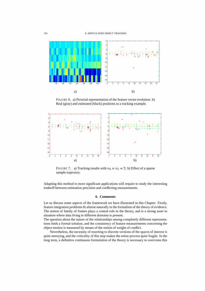
130 8. ARTICULATED OBJECT TRACKING
a) b)
FIGURE 6. a) Pictorial representation of the feature vector evolution. b)Real (gray) and estimated (black) positions in a tracking example.
a) b)
FIGURE 7. a) Tracking results with � � � � � � �. b) Effect of a sparse
sample trajectory.
Adapting this method to more significant applications will require to study the interestingtradeoff between estimation precision and conflicting measurements.
6. Comments
Let us discuss some aspects of the framework we have illustrated in this Chapter. Firstly,feature integration problems fit almost naturally in the formalism of the theory of evidence.The notion of family of frames plays a central role in the theory, and is a strong asset insituation where data living in different domains is present.The question about the nature of the relationships among completely different representa-tions finds a formal solution, and the consistency of feature measurements concerning theobject motion is measured by means of the notion of weight of conflict.
Nevertheless, the necessity of resorting to discrete versions of the spaces of interest isquite annoying, and the criticality of this step makes the entire process quite fragile. In thelong term, a definitive continuous formulation of the theory is necessary to overcome this
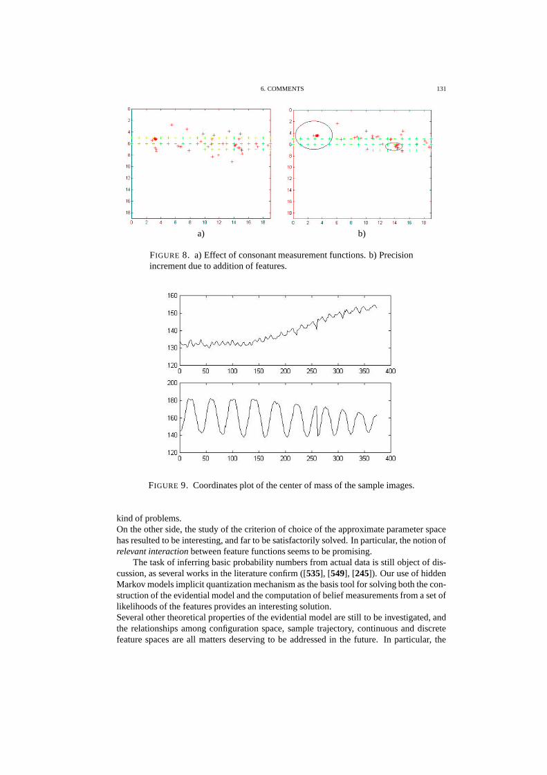
6. COMMENTS 131
a) b)
FIGURE 8. a) Effect of consonant measurement functions. b) Precisionincrement due to addition of features.
FIGURE 9. Coordinates plot of the center of mass of the sample images.
kind of problems.On the other side, the study of the criterion of choice of the approximate parameter spacehas resulted to be interesting, and far to be satisfactorily solved. In particular, the notion ofrelevant interaction between feature functions seems to be promising.
The task of inferring basic probability numbers from actual data is still object of dis-cussion, as several works in the literature confirm ([535], [549], [245]). Our use of hiddenMarkov models implicit quantization mechanism as the basis tool for solving both the con-struction of the evidential model and the computation of belief measurements from a set oflikelihoods of the features provides an interesting solution.Several other theoretical properties of the evidential model are still to be investigated, andthe relationships among configuration space, sample trajectory, continuous and discretefeature spaces are all matters deserving to be addressed in the future. In particular, the

132 8. ARTICULATED OBJECT TRACKING
pointwise estimation mechanism must be checked in more complex situations like high-dimensional non-linearly connected parameter spaces for ensuring the estimate to fall in
� .About the results, the analysis of the influence of the number of states of the discretized
feature spaces on tracking precision has shown that relatively rough discretizations canproduce appreciable outcomes.An interesting line of research could be the integration of our feature-based frameworkwith analytical model-based approaches ([375], [376]) to object tracking. The knowledgeof the kinematic model of the object, for example, could lower the estimate sensitivity tothe detail level of representations.
CHAPTER 9
Towards unsupervised action recognition
In the last two Chapters we have discussed the application of the theory of evidence toestimation problems. We want here to illustrate a classical classification-decision problemof computer vision that goes under the name of action recognition, with the major variantsof gesture and face recognition.In this context the machine, by processing measurements extracted from a sequence ofimages (typically under restrictive conditions), must be able to recognize the presence of acategory of motions it learned in advance. The choice of the features to be extracted fromthe images is crucial, for only a few details usually signal the presence of a particular kindof gesture, while the rest of the information is simply neglected. Unfortunately, withoutprior knowledge about the nature of the object in motion is very difficult to decide what isthe relevant information, for it is strictly dependent on the actual issue.It is then natural to imagine a framework in which the evidence produced by the analysis ofeach category of feature, typically a likelihood produced by a finite-state stochastic model,is pooled in a probable reasoning stage in order to make a decision.
In this Chapter we will then present a general model of an “action”, which will there-fore give it a precise definition, that includes both the dynamical and photometric char-acterization of the motion. All of its components, including feature representations, arepart of the action and must be constructed from the data. Invariance with respect to theparameters of the motion is guaranteed by both the global geometric representation andthe stochastic model of dynamics. We will adopt the formalism of hidden Markov models(introduced in Chapter 8) as a method for extracting the invariant dynamic pattern from acollection of instances of the action, avoiding the discretization of entire feature trajecto-ries.We will show that the model has compositional properties, in the sense that a model of asimple action can be detected from the model of a more complex one (in a dynamic “fore-ground + clutter” scenario), by showing how the model of a simple action can be recoveredfrom cluttered sequences.Finally, we will depict the future developments of our approach to unsupervised recog-nition and describe the role of the evidential reasoning in a completed system, in whichthe evidence resulting from the analysis of each feature or family of features is pooled bymeans of the Dempster-Shafer fusion scheme.
1. Action recognition in unsupervised context
Interpreting dynamic scenes, from the detection of a moving prey to the recognition of afriendly gesture, is crucial in the life of animals and remains one of the most important andyet largely untapped problems in computer vision. The problem is difficult because of thelarge variability in visual measurements of the same “action”: the appearance of a personwalking changes dramatically depending on pose, gait, clothing, age, as well as upon thephotometric, geometric and dynamical properties of the surrounding clutter. A model of
133
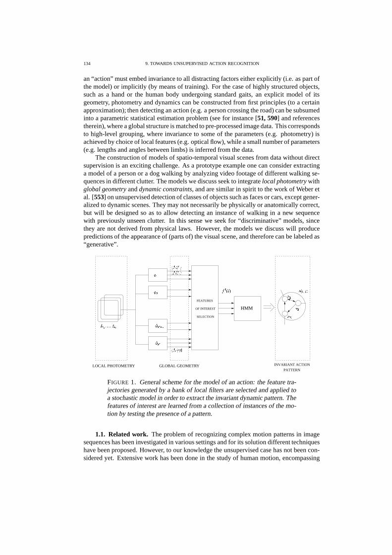
134 9. TOWARDS UNSUPERVISED ACTION RECOGNITION
an “action” must embed invariance to all distracting factors either explicitly (i.e. as part ofthe model) or implicitly (by means of training). For the case of highly structured objects,such as a hand or the human body undergoing standard gaits, an explicit model of itsgeometry, photometry and dynamics can be constructed from first principles (to a certainapproximation); then detecting an action (e.g. a person crossing the road) can be subsumedinto a parametric statistical estimation problem (see for instance [51, 590] and referencestherein), where a global structure is matched to pre-processed image data. This correspondsto high-level grouping, where invariance to some of the parameters (e.g. photometry) isachieved by choice of local features (e.g. optical flow), while a small number of parameters(e.g. lengths and angles between limbs) is inferred from the data.
The construction of models of spatio-temporal visual scenes from data without directsupervision is an exciting challenge. As a prototype example one can consider extractinga model of a person or a dog walking by analyzing video footage of different walking se-quences in different clutter. The models we discuss seek to integrate local photometry withglobal geometry and dynamic constraints, and are similar in spirit to the work of Weber etal. [553] on unsupervised detection of classes of objects such as faces or cars, except gener-alized to dynamic scenes. They may not necessarily be physically or anatomically correct,but will be designed so as to allow detecting an instance of walking in a new sequencewith previously unseen clutter. In this sense we seek for “discriminative” models, sincethey are not derived from physical laws. However, the models we discuss will producepredictions of the appearance of (parts of) the visual scene, and therefore can be labeled as“generative”.
HMM
SELECTION
OF INTEREST
FEATURES
INVARIANT ACTION
PATTERN
� � � � � � � � � � �
���
�����
� �
���
� � � � � � �� � � � � � �
� � ��� � � �
LOCAL PHOTOMETRY
���� � �
���� �
� �! � " # $%�
GLOBAL GEOMETRY
FIGURE 1. General scheme for the model of an action: the feature tra-jectories generated by a bank of local filters are selected and applied toa stochastic model in order to extract the invariant dynamic pattern. Thefeatures of interest are learned from a collection of instances of the mo-tion by testing the presence of a pattern.
1.1. Related work. The problem of recognizing complex motion patterns in imagesequences has been investigated in various settings and for its solution different techniqueshave been proposed. However, to our knowledge the unsupervised case has not been con-sidered yet. Extensive work has been done in the study of human motion, encompassing
2. REPRESENTATION OF ACTIONS 135
facial expression analysis [146, 39, 147], hand gesture recognition and whole-body track-ing (see [164] for a survey).A common approach consists of extracting low-level features by local spatio-temporal fil-tering on the images and using hidden Markov models (HMMs) on the collection of se-quences of points thus obtained for recognition and classification tasks [503, 563]. In[564], parametric HMMs are introduced for recognizing gestures that exhibit dependenceon a set of parameters, and in [50] coupled HMMs are used for modeling interactionsof two mobile objects. In [215], more complex actions are recognized by computing theprobability of a sequence of elementary actions detected by HMMs with a stochastic prob-abilistic parsing algorithm.In the literature, other statistical models, such as Bayesian Networks, are also used [323,36]. For complex actions, context-sensitive [362, 337] and multi-agent models [210] havebeen proposed. Some methods are based on optical flow. For each frame the flow canbe approximated with a small dimensional vector in suitable basis, as in [198], and therecognition done with HMMs as before, or, as in [40], a spatio-temporal representationof the optical flow can be built. In [168], a biological motion pattern is represented by alinear combination of prototypical image sequences. Other methods, such as in [51], use astatistical hierarchical approach based on local appearance.
2. Representation of actions
A satisfactory definition of the concept of “action” requires an accurate analysis of theproblem to avoid restrictive or simply ill-posed assumptions. First, the meaning of a mo-tion is often not associated to the entire trajectory but is summarized by a few significantportions of it. For instance, in a pointing gesture the crucial part is the arm reaching asteady, extended position for a while, no matter what trajectory it follows. Hence, trying toreproduce or parameterize the nuisance variability of a class of trajectories leads to fragilemodels and extremely difficult recognition. What we have to detect is the invariant patternalways present in every instance of the action.Even more important, the meaning of the action can be associated to different aspects ofthe movement. For instance, periodicity (closing the hand just once does not mean “bye!”),shape variations (e.g. hand gestures), critical configurations (the pointing gesture again),spatial trajectories (e.g. drawing). Therefore, in an unsupervised framework choosing afeature representing only a part of the information of the image sequence can generate anunacceptable bias. Finally, many actions are associated to movements of only one part ofan evolving object (locality). For instance, a walking person is free to move the upper partof the body.
In order to recognize actions, we need to define them as entities that can be easilydetected from sequences of images. From the above discussion this will require the intro-duction of a model both capturing an action by its photometric, geometric and dynamicinvariants, respecting the constraints of locality, and allowing the learning of the set offeatures characteristic of the action.
2.1. A three-level generative model. Consider a sequence of images� � � � ��� � � �������"��� � � ������� #where � � ) �
��� � is a positive array with a certain number of rows�
and columns
�. Let��� � � � � � ����� � # be a number of spatial or spatio-temporal filters (linear or non-linear),
that is� � � � � � � � where �
�is a subset of the image lattice. In the case of a spatio-
temporal filter,� � � � � � �
�� � � where �
�is a subset of the time set
� �� � � ����������# .

136 9. TOWARDS UNSUPERVISED ACTION RECOGNITION
��� � � � � � ����� � # could be a linear filter banks, a multi-scale family of oriented filters,or even a global filter, for instance the so-called “size functions” ([159]), or inter-frameoptical flow [16].
The location of the maximal response of each filter changes, in general, during thesequence, so that we have a set of trajectories
� � � � � � � � ��� ����� � � � ��� � � ��������# , which wecall feature trajectories. Only some of the feature trajectories will be of interest; we callthe others the “background scene”; portions of feature trajectories may be missing.
We assume that feature trajectories of interest describe smooth transitions between acertain number � of configurations of maximal responses of filters
����� � � � � ����� � # ,which we call feature configurations. Feature configurations are organized into a graphwhere
���are the nodes, and edges represent the probability of a smooth transitions from
one configuration to another. Such a graph represents an invariant pattern that can beextracted from every instance of the action, and does not necessarily encode the wholefeature trajectories.
This model can be thought of as a three-level generative stochastic model. At thehighest level we have actions, which are defined as stochastic automata of feature con-figurations. At the intermediate level we have feature trajectories mixed with clutter anddistractors. At the lowest level we have photometric patterns evolving in time on the im-age plane. This is illustrated by figure 1. The three levels correspond roughly to localphotometry (lowest) to global geometry (intermediate), to discrete indexing (highest).
2.2. Learning actions. As stochastic representation of the transitions between fea-ture configuration we adopted the formalism of hidden Markov model. In Chapter 8, Sec-tion 1.2 we have seen the basic features of this class of models. We just want to notethat we use an application of the EM technique that is slightly different from the classicalBaum-Welch procedure and is based on a one-pass [143] iterative update of the matrices.
As we mentioned above, in order to specify an action we need to give a description ofeach level, including the choice of filters
� �, feature poses
��
and the dynamics encodedby the transition matrix � � � � � � .Now, making the assumption that the “correct” filters are given, HMMs provide a methodto build the invariant pattern or graph between feature configurations, giving the sequenceof feature observations extracted from the images as input of its learning algorithm. Theparameters of the resulting model will then encode the feature configurations as columnsof the
�matrix, and their dynamics as transition probabilities in the � matrix.
It is interesting to remark that invariance to execution speed is embedded in the HMMrepresentation once the auto-transitions of the states are neglected.
3. Detecting actions in clutter
We want to test the compositional property of the model we described above, by showingthat it is possible to recover the invariant pattern from the model of a complex motion.
3.1. Clustering. Our fundamental claim is that there exists a choice of features underwhich the model of an action in clutter is embedded into the model of the cluttered motion.In other words, there is a map between the model representing a sequence containing bothforeground and background motion and the model of the action of interest. We need tomake the nature of this map precise, find a way of extracting the invariant informationfrom an HMM built from a cluttered sequence and a criterion to compare the extractedinformation with the learned model of the action of interest.
Now let us suppose that we are given the suitable family of local features.
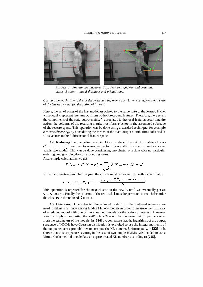
3. DETECTING ACTIONS IN CLUTTER 137
FIGURE 2. Feature computation. Top: feature trajectory and boundingboxes. Bottom: mutual distances and orientations.
Conjecture: each state of the model generated in presence of clutter corresponds to a stateof the learned model for the action of interest.
Hence, the set of states of the first model associated to the same state of the learned HMMwill roughly represent the same positions of the foreground features. Therefore, if we selectthe components of the state-output matrix
�associated to the local features describing the
action, the columns of the resulting matrix must form clusters in the associated subspaceof the feature space. This operation can be done using a standard technique, for examplek-means clustering, by considering the means of the state-output distributions collected in�
as vectors in the d-dimensional feature space.
3.2. Reducing the transition matrix. Once produced the set of � � state clusters+ � � � � �� ��� � � � � �� � # we need to rearrange the transition matrix in order to produce a new
admissible model. This can be done considering one cluster at a time with no particularordering, and grouping the corresponding states.After simple calculations we get
����� � � �) + � � � � � � � � �
� � � �� ����� � � �
� � � � � � � � � �while the transition probabilities from the cluster must be normalized with its cardinality:
����� � � �� � � � � � ) + � � � � � � � �
� ����� � � �� � � � � � � � � �� + � � �
This operation is repeated for the next cluster on the new � until we eventually get an� � � � � matrix. Finally the columns of the reduced � must be permuted to match the orderthe clusters in the reduced
�matrix.
3.3. Detection. Once extracted the reduced model from the cluttered sequence weneed to define a distance among hidden Markov models in order to measure the similarityof a reduced model with one or more learned models for the action of interest. A naturalway to comply is computing the Kullback-Leibler number between their output processesfrom the parameters of the models. In [516] the conjecture that the logarithms of the outputsequence of HMMs have Gaussian distribution is exploited to use the integer moments ofthe output sequence probabilities to compute the KL number. Unfortunately, in [226] it isshown that this conjecture is wrong in the case of two simple HMMs. We decided to use aMonte-Carlo method to calculate an approximated KL number, according to [225].
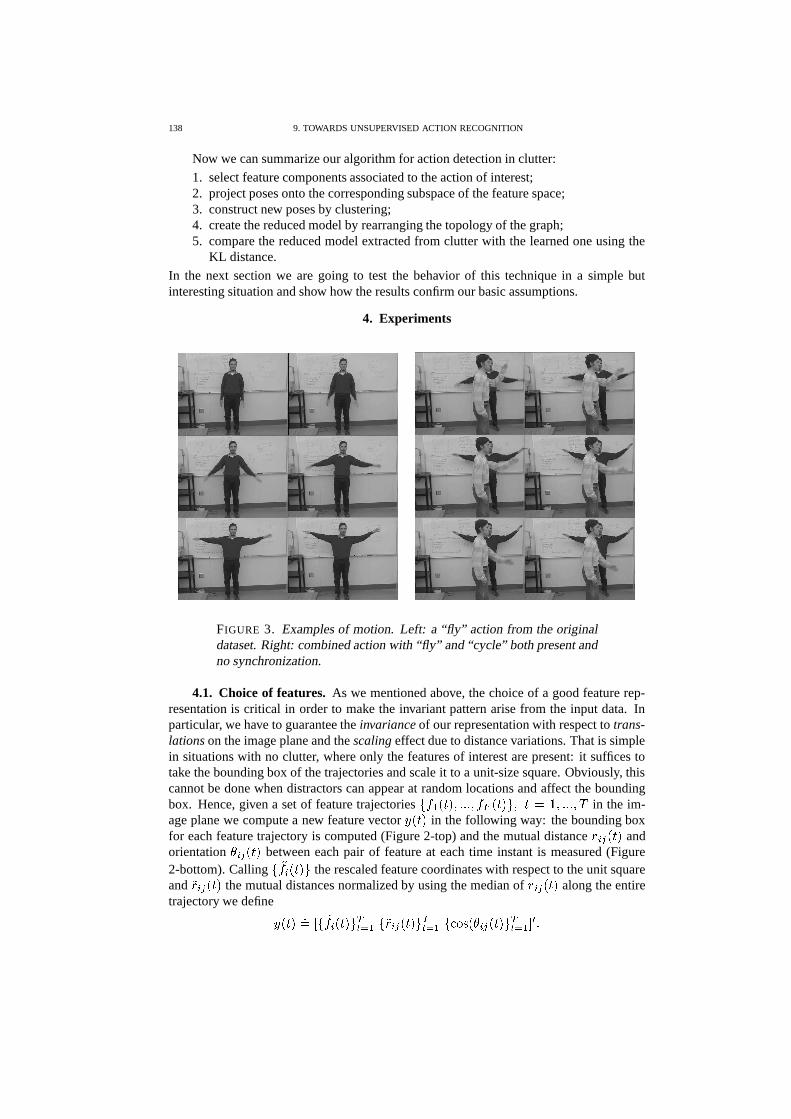
138 9. TOWARDS UNSUPERVISED ACTION RECOGNITION
Now we can summarize our algorithm for action detection in clutter:
1. select feature components associated to the action of interest;2. project poses onto the corresponding subspace of the feature space;3. construct new poses by clustering;4. create the reduced model by rearranging the topology of the graph;5. compare the reduced model extracted from clutter with the learned one using the
KL distance.
In the next section we are going to test the behavior of this technique in a simple butinteresting situation and show how the results confirm our basic assumptions.
4. Experiments
FIGURE 3. Examples of motion. Left: a “fly” action from the originaldataset. Right: combined action with “fly” and “cycle” both present andno synchronization.
4.1. Choice of features. As we mentioned above, the choice of a good feature rep-resentation is critical in order to make the invariant pattern arise from the input data. Inparticular, we have to guarantee the invariance of our representation with respect to trans-lations on the image plane and the scaling effect due to distance variations. That is simplein situations with no clutter, where only the features of interest are present: it suffices totake the bounding box of the trajectories and scale it to a unit-size square. Obviously, thiscannot be done when distractors can appear at random locations and affect the boundingbox. Hence, given a set of feature trajectories
� ��� � � ��� � � � ��� � � � #�� � � � ��� � � � � in the im-
age plane we compute a new feature vector� � � � in the following way: the bounding box
for each feature trajectory is computed (Figure 2-top) and the mutual distance� � � � � � and
orientation � � � � � � between each pair of feature at each time instant is measured (Figure2-bottom). Calling
� �� � � � � # the rescaled feature coordinates with respect to the unit squareand
�� � � � � � the mutual distances normalized by using the median of� � � � � � along the entire
trajectory we define� � � � �� � � �� � � � � # �� 6 �
� �� � � � � � # �� 6 ���� � � � � � � � � � # �� 6 �
! � �
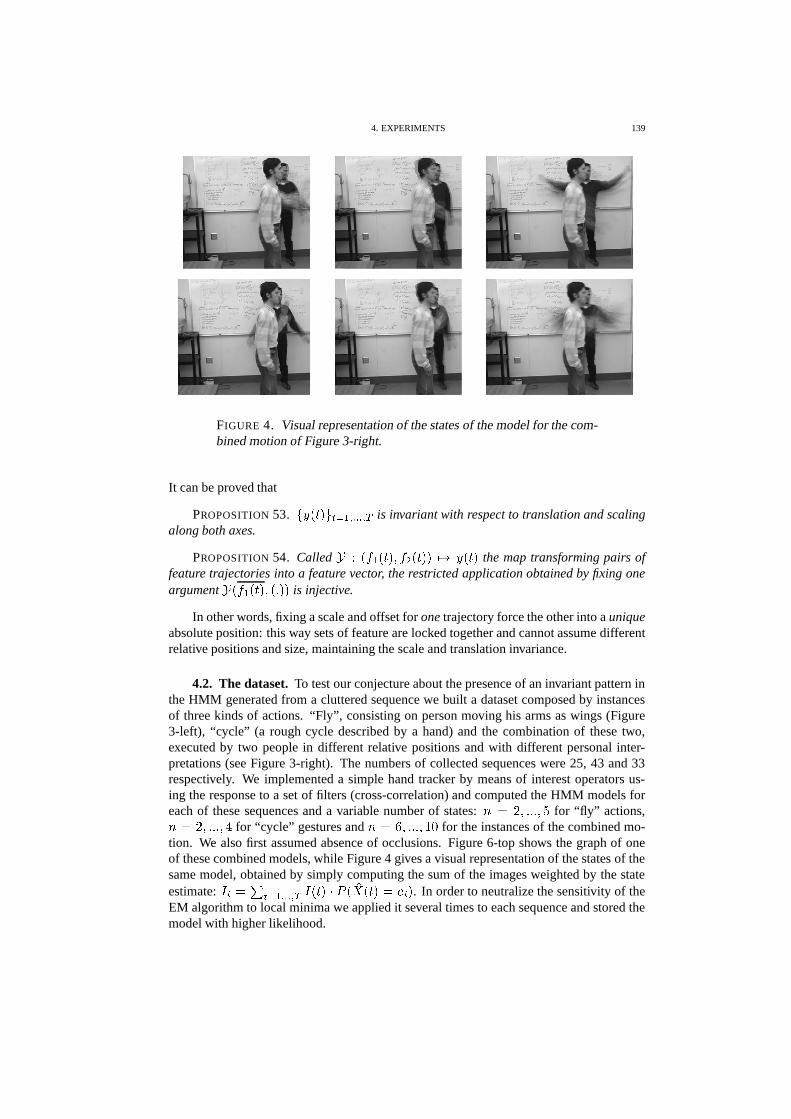
4. EXPERIMENTS 139
FIGURE 4. Visual representation of the states of the model for the com-bined motion of Figure 3-right.
It can be proved that
PROPOSITION 53.� � � � � # � 6 � � � � � is invariant with respect to translation and scaling
along both axes.
PROPOSITION 54. Called� � � � �
� � � � � � � � � � �� � � � � the map transforming pairs offeature trajectories into a feature vector, the restricted application obtained by fixing oneargument
� � ��� � �"� � � � � is injective.
In other words, fixing a scale and offset for one trajectory force the other into a uniqueabsolute position: this way sets of feature are locked together and cannot assume differentrelative positions and size, maintaining the scale and translation invariance.
4.2. The dataset. To test our conjecture about the presence of an invariant pattern inthe HMM generated from a cluttered sequence we built a dataset composed by instancesof three kinds of actions. “Fly”, consisting on person moving his arms as wings (Figure3-left), “cycle” (a rough cycle described by a hand) and the combination of these two,executed by two people in different relative positions and with different personal inter-pretations (see Figure 3-right). The numbers of collected sequences were 25, 43 and 33respectively. We implemented a simple hand tracker by means of interest operators us-ing the response to a set of filters (cross-correlation) and computed the HMM models foreach of these sequences and a variable number of states: � � � ��� � � � � for “fly” actions,� � � ��� � � � � for “cycle” gestures and � � � ��� � � � � � for the instances of the combined mo-tion. We also first assumed absence of occlusions. Figure 6-top shows the graph of oneof these combined models, while Figure 4 gives a visual representation of the states of thesame model, obtained by simply computing the sum of the images weighted by the stateestimate: �
� � � � 6 � � � � � � � � � ��� �� � � � � � � � . In order to neutralize the sensitivity of theEM algorithm to local minima we applied it several times to each sequence and stored themodel with higher likelihood.
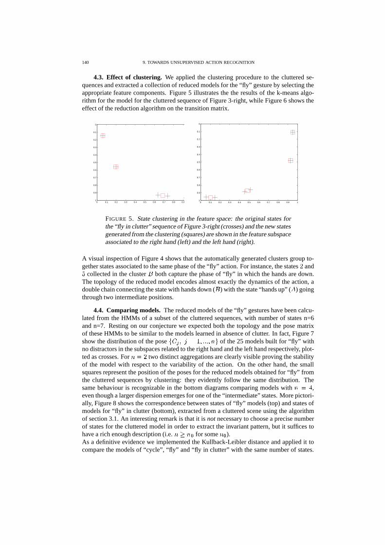
140 9. TOWARDS UNSUPERVISED ACTION RECOGNITION
4.3. Effect of clustering. We applied the clustering procedure to the cluttered se-quences and extracted a collection of reduced models for the “fly” gesture by selecting theappropriate feature components. Figure 5 illustrates the the results of the k-means algo-rithm for the model for the cluttered sequence of Figure 3-right, while Figure 6 shows theeffect of the reduction algorithm on the transition matrix.
0 0.1 0.2 0.3 0.4 0.5 0.6 0.7 0.8 0.9 1
0
0.1
0.2
0.3
0.4
0.5
0.6
0.7
0.8
0.9
10 0.1 0.2 0.3 0.4 0.5 0.6 0.7 0.8 0.9 1
0
0.1
0.2
0.3
0.4
0.5
0.6
0.7
0.8
0.9
1
FIGURE 5. State clustering in the feature space: the original states forthe “fly in clutter” sequence of Figure 3-right (crosses) and the new statesgenerated from the clustering (squares) are shown in the feature subspaceassociated to the right hand (left) and the left hand (right).
A visual inspection of Figure 4 shows that the automatically generated clusters group to-gether states associated to the same phase of the “fly” action. For instance, the states � and� collected in the cluster
�both capture the phase of “fly” in which the hands are down.
The topology of the reduced model encodes almost exactly the dynamics of the action, adouble chain connecting the state with hands down (
�) with the state “hands up” ( � ) going
through two intermediate positions.
4.4. Comparing models. The reduced models of the “fly” gestures have been calcu-lated from the HMMs of a subset of the cluttered sequences, with number of states n=6and n=7. Resting on our conjecture we expected both the topology and the pose matrixof these HMMs to be similar to the models learned in absence of clutter. In fact, Figure 7show the distribution of the pose
� � � � � � � ��� � � �!��# of the 25 models built for “fly” withno distractors in the subspaces related to the right hand and the left hand respectively, plot-ted as crosses. For � � � two distinct aggregations are clearly visible proving the stabilityof the model with respect to the variability of the action. On the other hand, the smallsquares represent the position of the poses for the reduced models obtained for “fly” fromthe cluttered sequences by clustering: they evidently follow the same distribution. Thesame behaviour is recognizable in the bottom diagrams comparing models with � � � ,even though a larger dispersion emerges for one of the “intermediate” states. More pictori-ally, Figure 8 shows the correspondence between states of “fly” models (top) and states ofmodels for “fly” in clutter (bottom), extracted from a cluttered scene using the algorithmof section 3.1. An interesting remark is that it is not necessary to choose a precise numberof states for the cluttered model in order to extract the invariant pattern, but it suffices tohave a rich enough description (i.e. � � � 7 for some � 7 ).As a definitive evidence we implemented the Kullback-Leibler distance and applied it tocompare the models of “cycle”, “fly” and “fly in clutter” with the same number of states.
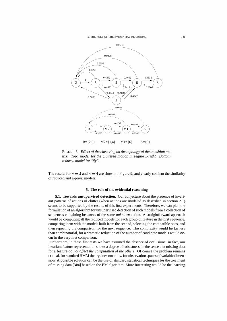
5. THE ROLE OF THE EVIDENTIAL REASONING 141
5 6 3
1
2 4
0.5058
1
0.93060.4652
0.4373 0.24180.4942
0.2418
0.4373 0.4652 0.4836
0.0328
0.0696
0.1253
0.0694
B M1 A1
0.5265
0.4735 0.4836
0.4836 0.9306
0.0328
0.0694
M2
B={2,5} M2={1,4} M1={6} A={3}
FIGURE 6. Effect of the clustering on the topology of the transition ma-trix. Top: model for the cluttered motion in Figure 3-right. Bottom:reduced model for “fly”.
The results for � � � and � � � are shown in Figure 9, and clearly confirm the similarityof reduced and a-priori models.
5. The role of the evidential reasoning
5.1. Towards unsupervised detection. Our conjecture about the presence of invari-ant patterns of actions in clutter (when actions are modeled as described in section 2.1)seems to be supported by the results of this first experiments. Therefore, we can plan theformulation of an algorithm for unsupervised detection of such models from a collection ofsequences containing instances of the same unknown action. A straightforward approachwould be computing all the reduced models for each group of feature in the first sequence,comparing them with the models built from the second, selecting the compatible ones, andthen repeating the comparison for the next sequence. The complexity would be far lessthan combinatorial, for a dramatic reduction of the number of candidate models would oc-cur in the very first comparison.Furthermore, in these first tests we have assumed the absence of occlusions: in fact, ourinvariant feature representation shows a degree of robustness, in the sense that missing datafor a feature do not affect the computation of the others. Of course the problem remainscritical, for standard HMM theory does not allow for observation spaces of variable dimen-sion. A possible solution can be the use of standard statistical techniques for the treatmentof missing data [304] based on the EM algorithm. More interesting would be the learning
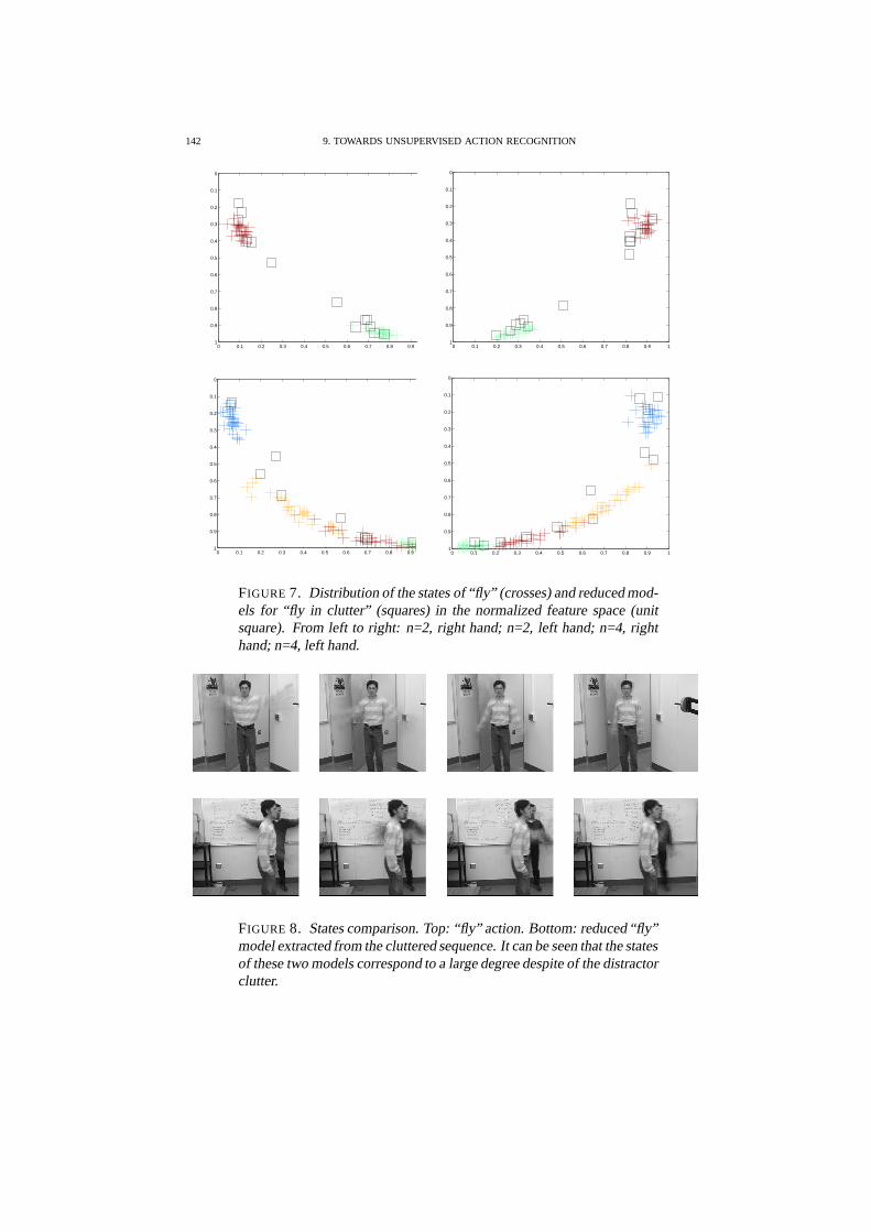
142 9. TOWARDS UNSUPERVISED ACTION RECOGNITION
0 0.1 0.2 0.3 0.4 0.5 0.6 0.7 0.8 0.9 1
0
0.1
0.2
0.3
0.4
0.5
0.6
0.7
0.8
0.9
10 0.1 0.2 0.3 0.4 0.5 0.6 0.7 0.8 0.9 1
0
0.1
0.2
0.3
0.4
0.5
0.6
0.7
0.8
0.9
1
0 0.1 0.2 0.3 0.4 0.5 0.6 0.7 0.8 0.9 1
0
0.1
0.2
0.3
0.4
0.5
0.6
0.7
0.8
0.9
10 0.1 0.2 0.3 0.4 0.5 0.6 0.7 0.8 0.9 1
0
0.1
0.2
0.3
0.4
0.5
0.6
0.7
0.8
0.9
1
FIGURE 7. Distribution of the states of “fly” (crosses) and reduced mod-els for “fly in clutter” (squares) in the normalized feature space (unitsquare). From left to right: n=2, right hand; n=2, left hand; n=4, righthand; n=4, left hand.
FIGURE 8. States comparison. Top: “fly” action. Bottom: reduced “fly”model extracted from the cluttered sequence. It can be seen that the statesof these two models correspond to a large degree despite of the distractorclutter.
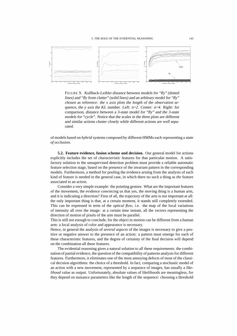
5. THE ROLE OF THE EVIDENTIAL REASONING 143
0 2 4 6 8 10 12 14 16 18 200
0.5
1
1.5
2
2.5
3
Observation sequence length
K−
L di
stan
ce
0 2 4 6 8 10 12 14 16 18 200
1
2
3
4
5
6
7
Observation sequence length
K−
L di
stan
ce
0 2 4 6 8 10 12 14 16 18 200
5
10
15
20
25
30
35
Observation sequence length
K−
L di
stan
ce
fly
cycle
FIGURE 9. Kullback-Leibler distance between models for “fly” (dottedlines) and “fly from clutter” (solid lines) and an arbitrary model for “fly”chosen as reference: the x axis plots the length of the observation se-quence, the y axis the KL number. Left: n=2. Center: n=4. Right: forcomparison, distance between a 3-state model for “fly” and the 3-statemodels for “cycle”. Notice that the scales in the three plots are differentand similar actions cluster closely while different actions are well sepa-rated.
of models based on hybrid systems composed by different HMMs each representing a stateof occlusion.
5.2. Feature evidence, fusion scheme and decision. Our general model for actionsexplicitly includes the set of characteristic features for that particular motion. A satis-factory solution to the unsupervised detection problem must provide a reliable automaticfeature selection stage, based on the presence of the invariant pattern in the correspondingmodels. Furthermore, a method for pooling the evidence arising from the analysis of eachkind of feature is needed in the general case, in which there no such a thing as the featureassociated to an action.
Consider a very simple example: the pointing gesture. What are the important featuresof the movement, the evidence convincing us that yes, the moving thing is a human arm,and it is indicating a direction? First of all, the trajectory of the arm is not important at all:the only important thing is that, at a certain moment, it stands still completely extended.This can be expressed in term of the optical flow, i.e. the map of the local variationsof intensity all over the image: at a certain time instant, all the vectors representing thedirection of motion of pixels of the arm must be parallel.This is still not enough to conclude, for the object in motion can be different from a humanarm: a local analysis of color and appearance is necessary.Hence, in general the analysis of several aspects of the images is necessary to give a pos-itive or negative answer to the presence of an action: a pattern must emerge for each ofthese characteristic features, and the degree of certainty of the final decision will dependon the combination all these features.
The evidential reasoning gives a natural solution to all these requirements: the combi-nation of partial evidence, the question of the compatibility of patterns analysis for differentfeatures. Furthermore, it eliminates one of the most annoying defects of most of the classi-cal decision algorithms: the choice of a threshold. In fact, comparing a stochastic model ofan action with a new movement, represented by a sequence of images, has usually a like-lihood value as output. Unfortunately, absolute values of likelihoods are meaningless, forthey depend on nuisance parameters like the length of the sequence: choosing a threshold
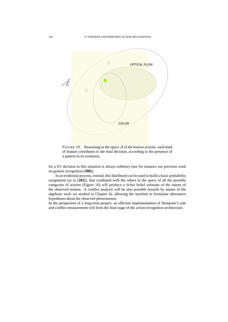
144 9. TOWARDS UNSUPERVISED ACTION RECOGNITION
FIGURE 10. Reasoning in the space�
of the known actions: each kindof feature contributes to the final decision, according to the presence ofa pattern in its evolution.
for a 0/1 decision in this situation is always arbitrary (see for instance our previous workon gesture recognition [498]).
In an evidential process, instead, this likelihood can be used to build a basic probabilityassignment (as in [282]), that combined with the others in the space of all the possiblecategories of actions (Figure 10) will produce a richer belief estimate of the nature ofthe observed motion. A conflict analysis will be also possible (maybe by means of thealgebraic tools we studied in Chapter 6), allowing the machine to formulate alternativehypotheses about the observed phenomenon.In the perspective of a long-term project, an efficient implementation of Dempster’s ruleand conflict measurement will form the final stage of the action recognition architecture.

Part 4
Conclusions and appendices

CHAPTER 10
Conclusions
As we mentioned at the beginning, the aim of this thesis was not to claim that thegeneralization of probability theory emerging from the work of Dempster and Shafer, butalso Kohlas, Smets and others, is the right way to cope with the practical problems arisingin computer vision that involve deductions, or estimations, in a context of uncertainty. Aswe have largely shown in the extensive review of Chapter 3, the debate on the philosophi-cal motivations at the basement of uncertainty theory is also intense, and the most popularopinion seems to support the idea that there is no an ultimate formalism suitable to everysituation. We are not going to partecipate to this debate, that is beyond the goals of thiswork.Instead, we hope we have given a flavor of the richness of the theory of evidence, in termsof its applicability to a large number of problems (in particular computer vision ones), andof the emerging of interesting theoretical questions due to the greater “internal structure”belief functions have when compared to classical probabilities.It is worth to point out that all the theoretical issues we presented here are direct conse-quences of the formulation of evidential solutions to the vision applications of Chapter 7and Part III, which have been shown later only for “didactic” purposes.
The number of open problems is huge, and only a brief hint to some of them is possiblehere in this final considerations.
The geometric analysis exposed in Chapter 4 is clearly only at its initial stage, evenif some interesting results have been achieved. We now have a picture of the behavior ofbelief functions as geometrical objects, but the questions that has motivated this approachstill need to be addressed. A general expression of the consonant and probabilistic approx-imations of a belief functions, based on the principle of “external” behavior we have seenin Section 9, is to be found.The language we introduced, based on the commutativity of Dempster’s rule and convexclosure seems to be very promising, especially concerning the derivation of the canonicaldecomposition of a generic separable support function. Encouraging partial results havealready been achieved, even if we did not include them in this thesis.
A collateral effect of the algebraic structure of the families of frames, given its strongbond to the idea of support function, could be a new interpretation of the families of com-patible support functions. This question is strictly connected to the possibility we hintedin Chapter 6 of solving the conflict problem by formulating a pseudo Gram-Schmidt algo-rithm.The problem of canonical decomposition, perhaps, could be approached from another pointof view by integrating the geometrical and algebraic frameworks, and studying the geomet-ric relations among belief spaces associated to compatible frames. An hint about the rightdirection to take is provided by the notion of lattice of convex hulls ([505]).
The notion of sequence of random variables or random process is perhaps the mostwidely used in almost all the engineering applications, including control engineering and
147
148 10. CONCLUSIONS
computer vision: it suffices to think about the role of the Kalman filter formalism. Theknowledge of the geometrical form of conditional subspaces could be used to predict thecharacteristics of series of belief functions� � �� ��� � � � � � � � � �$� �and their asymptotic properties, helping to start the study of the evidential analogous of arandom process.
The formulation of the total probability theorem we encountered in Chapter 7 is a goodstep towards a definitive description of the combination of conditional data in an evidentialframework. We have already started to explain what further actions may conduct to afinal arrangement of the matter. In the future, it will worth to investigate in more detailseveral different interesting alternative views of the total belief problem, that could be ableto enrich our knowledge of the theory of belief functions and its relation with unsuspectedfields of mathematics apparently alien to combinatorics.For instance, homology theory provides a natural environment in which to pose the graph-theoretic problem concerning the candidate total functions, and possibly find a generalizedtransformation class powerful enough to solve the general instance. In fact, the linearsystems associated to the candidate solutions form a simplicial complex(see [505] again),and the transformations representing the edges of a solution graph resemble the formal sumof a chain
� � � � � �where �
�is a k-dimensional simplex of the complex and
� ) � is an arbitrary element ofa group G.On the other hand, conditional subspaces establish a connection between the operations ofconditioning with respect to functions and events. It suffices to remember that
� � � �� � � � � � ( �'� � +-, �
where
� � � ( � � � (is the belief function � conditioned by the event � . This way the total evidence issue canbe formulated as a geometric problem too.
Finally, engineers could spot the appeal of an interpretation of the nature of candi-date solutions in term of positive systems. The link easily appears when one compares thegraphical layout of a candidate solution with the influence graphs of linear systems withall positive coefficients, but the same result can be obtained by rearranging their coeffi-cient matrices into a matrix with � � � coefficients. Elegant results could then be reachedby expressing problems concerning conditional generalized probabilities as well-knownsystem-theoretic issues such as, for instance, controllability.
Among the applications, the evidential model we introduced as a solution to objecttracking is particularly interesting, for it involves several critical questions. The most im-portant, perhaps, is the formulation of a definitive criterion for the discretization of theparameter space, which is bonded to the idea of relevant interaction of continuous fea-tures, a promising one in the perspective of a continuous theory of evidence.The asymptotic behaviour of the evidential model for increasing refinements of the pa-rameter space, with particular attention to the conflict among data, is another unsolvedpuzzle that is worth to face, in order to analyze the dependence of the estimate from thediscretization of the parameter space.
10. CONCLUSIONS 149
An interesting application of the object tracking framework could be the situation inwhich the articulated object is a human hand (hand tracking), a significant case for its largenumber of degrees of freedom. Standard kinematic models of the hand[376] has been usedto solve this problem: we think that the integration of the evidential model of the objectwith a kinematic model can improve both robustness and tracking precision, allowing theextension of our estimation method to high-dimensional non-convex parameter spaces.
In a long term perspective, it will be fundamental to detect a “benchmark” applica-tion, to be used for a comprehensive comparison of the performances of probabilistic andevidential approaches: that could help us to understand limits and potentialities of the the-ory of evidence. The data association problem meets these requirements, and certainlydeserves a further deepening.


APPENDIX A
Algebraic structures
1. Posets and lattices
DEFINITION 52. A chain of a poset is a collection of consecutive elements; two ele-ments � � � are consecutive if � � � (or � � � ) and
� � � s.t. � � � � � ( � � � � � ).
DEFINITION 53. A poset is called a finite length poset if the length of its chains islimited.
DEFINITION 54. A poset is said to have locally finite length is each of its intervalsconsidered as posets have finite length.
DEFINITION 55. A lattice is a poset in which any arbitrary finite collection� � � ��� � � ��� � #
of elements admits a greatest lower bound ( � ��� )�
and a smallest upper bound ( ����� )�
.�and
�both satisfy the following properties:
1. associativity: � � � � � � � � � � � � � � � � � � � � � � � � � � � � � � � ;2. commutativity: � � � � � � � �'� � � � � � � ;3. idempotence: � � � � � � � � � � � ;4.
� � � � � � � � � � � � � � � � � � � .
1.1. Distributivity. In a lattice are equivalent:
� � � � � � � � � � �"� � � � � � � � � � � � � � � � � �"� � � � � ���(47)
DEFINITION 56. A lattice satisfying (47) is called distributive.
For example, every totally ordered set is a distributive lattice.
PROPOSITION 55. A sufficient condition for distributivity is
� � � � � � % � � � �"� � � � � � �the reverse inequality is indeed always satisfied.
The subspace lattice � � (� is not distributive.
1.2. Modularity.
DEFINITION 57. A lattice is modular when��� � � � � � � � � � � � � � � � � � � � � � � �"� � � � � � ���It obviously is a condition weaker than (47). Hence
PROPOSITION 56. If a lattice L is distributive then it is modular.
There is also an alternative definition of modularity.
DEFINITION 58. L is modular iff if � � � , � � � � � , � � � � � then � � � .
151
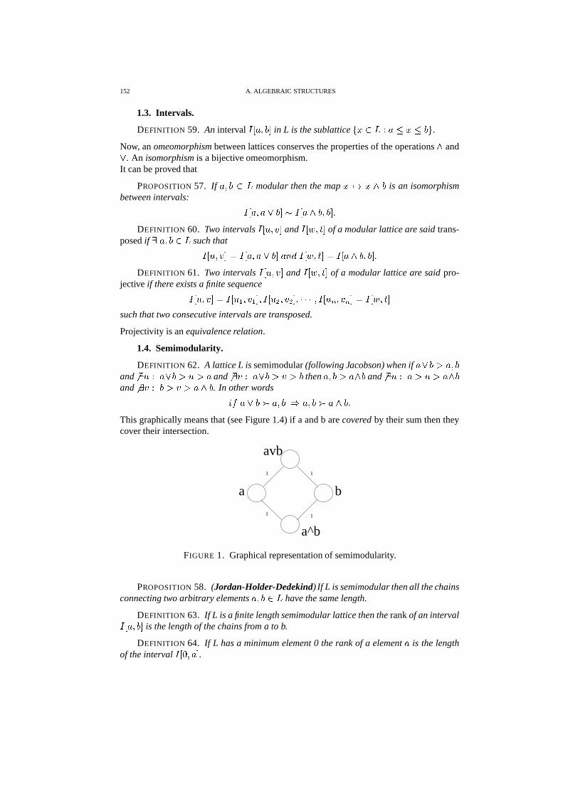
152 A. ALGEBRAIC STRUCTURES
1.3. Intervals.
DEFINITION 59. An interval � � � ��� ! in L is the sublattice��� ) � � � % � % �$# .
Now, an omeomorphism between lattices conserves the properties of the operations�
and�
. An isomorphism is a bijective omeomorphism.It can be proved that
PROPOSITION 57. If � ��� ) � modular then the map� �� � � � is an isomorphism
between intervals:
� � � � � � � ! �� � � � � ��� ! �DEFINITION 60. Two intervals � � � � � ! and � � �(� � ! of a modular lattice are said trans-
posed if � � ��� ) � such that
� � � � � ! � � � � � � � � ! ����� � � �(� � ! � � � � � � ��� ! �DEFINITION 61. Two intervals � � � � � ! and � � �(� � ! of a modular lattice are said pro-
jective if there exists a finite sequence
� � � � � ! � � � � � � � �! ��� � � � � ��� ! � � � � ��� � � � � ��� ! � � � �(� � !
such that two consecutive intervals are transposed.
Projectivity is an equivalence relation.
1.4. Semimodularity.
DEFINITION 62. A lattice L is semimodular (following Jacobson) when if � � � � � ���and
� � � � � � � � � � � and� � � � � � � � � � � then � ��� � � � � and
� � � � � � � � � � �and
� � � � � � � � � � � . In other words��� � � � � � ��� � � ��� � � � � �This graphically means that (see Figure 1.4) if a and b are covered by their sum then theycover their intersection.
a b
a^b
avb
1 1
11
FIGURE 1. Graphical representation of semimodularity.
PROPOSITION 58. (Jordan-Holder-Dedekind) If L is semimodular then all the chainsconnecting two arbitrary elements � ��� ) � have the same length.
DEFINITION 63. If L is a finite length semimodular lattice then the rank of an interval� � � ��� ! is the length of the chains from a to b.
DEFINITION 64. If L has a minimum element 0 the rank of a element � is the lengthof the interval � � � � � ! .
1. POSETS AND LATTICES 153
PROPOSITION 59. They are equivalent:# L is modular;# L and
�� are semimodular;# L satisfies the length chain rule and the ”condition on the rank”
� � � � �"� � � � � � � � � �"����� � � � �"���Let us see a significant application of these notions in order to clarify the difference amongdifferent kinds of lattices. When L is a semimodular bounded below lattice its elementsare characterized by a rank, nothing more than the length of the interval
� � � � � � � � � � ! .When L is even modular then the dimension rule holds
� � � � �"� � � � � � � � � �"����� � � � �"���(for it depends from the isomorphism � � � � � � � ! �� � � � � ��� ! ) If � and � are complementary
� � � � � � � � � �"����� � � � � � � � � � � � �"� � � � � � � � � � � � � �"� � � � � ����� � � �so that all the complements of a given element � must have the same rank and they cannotform a chain.
1.5. Complemented and relatively complemented lattices.
DEFINITION 65. A lattice bouded below and above is called complemented if
� � ) � � � � ) � ��� � � � � � � � � �'� � � � � � �� � is called complement of a.
For instance, � � � is a modular complemented lattice.Distributivity ensures the uniqueness of the complement. Anyway, the condition can berelaxed. Recurring to [216] we note that the proof depends on the following passage:
� �� � � � � � � � � � �
� � � � � � �� � � ���
Of course if L is distributive the above condition is satisfied, but it easy to see that isnecessary and sufficient that L is modular and � � � � or � � � � � . In other words
PROPOSITION 60. A lattice admits unique complements iff it is modular and there notexist intervals of distinct complements.
For instance, the lattice of subspaces � � (� of a projective space V is not distributive butnevertheless it admits only unique complements: given a subspace � we can detect itsorthogonal complement in V without ambiguity.We can now introduce an alternative definition of modularity.
DEFINITION 66. A lattice L is relatively complemented if each interval � � � ��� ! in L iscomplemented as a sublattice.
Obviously if L is relatively complemented then it is complemented too.
DEFINITION 67. The semicomplement of a element u is another element x such that
� � � � ���All the semicomplements of a given element u form a poset, with a maximal element
� 7 .Furthermore, if x is a semicomplement of u then
� � !are all semicomplements, too.
PROPOSITION 61. Complements in a complete lattice form an interval.
PROOF. Since they are semicomplements with respect to� � � ��� then they have the
form� � 7 ! for some
� 7 . At the same time they are semicomplements for� �� � � � so that they
must be of the form � � � � : the intersection of these sets is obviously an interval.

154 A. ALGEBRAIC STRUCTURES
1.6. Lattices bounded below and atoms.
DEFINITION 68. If L is a lattice bounded below then its atoms are the elements of Lcovering 0, namely
� � � � ) � � � � � #��1.7. Birkhoff lattices.
DEFINITION 69. The upper covering condition is � � � ��� � � � � � � .DEFINITION 70. The lower covering condition is � � � � � � � � � ��� .
Obviously if L satisfies both conditions then it is modular:
� � � � � � � � � � � �DEFINITION 71. A Birkhoff lattice is a finite length lattice that satisfies the lower
covering condition.
Of course every modular finite lattice is Birkhoff.
PROPOSITION 62. The following conditions are equivalent:# a Birkhoff lattice L is modular;# its dual
�� is modular;# � �&��� � � � � � � � � � �"� � � � � � �"� � � � � � �"� .DEFINITION 72. A lattice L is semimodular (following Szasz, [519]) when
� � ��� � � ��� � � � � � ����� � � � � � � � � � � � � � � � % � ����� � � � � � � � � � �Every semimodular lattice satisfies the lower covering condition so that
PROPOSITION 63. A finite length lattice is semimodular iff it is Birkhoff.
Remark. [519] and [216] use the same word (“semimodular”) with different mean-ings.
PROPOSITION 64. If a lattice meets the double covering condition then is a Jacobsonsemimodular lattice.
PROPOSITION 65. Let L be a finite length lattice. If it satisfies the lower coveringcondition
� � � � � � � �"� � � � � � �"� � � � � � �"� �if L satisfies the upper covering condition
� � � � � � � �"� % � � � � �"� � � � � � �"� �obviously if L meets both them it meets the dimension rule too.
2. Boolean algebras
The material of this section comes from Sikorski’s book [439].
DEFINITION 73. A Boolean algebra is a non-empty set�
provided with three internaloperations
� � � � � � �
�(� � �� � �� + � � � � � � �
�(� � �� �,+ � � � � � � �
� �� � �

2. BOOLEAN ALGEBRAS 155
called respectively meet, join and complement, characterized by the following properties:
� + � � � +��(� � �� � �� � � � � �
�,+ ��� +�� � � �,+ � � +
�� � ���
�� � � � �� �
�� �� �
� � �� � + � � � � � �,+ � � �� � � � � � �
� ��� +�� � � � � � + � �
�� � �,+ ����
�� � � �,+ � � � �,+
�� � � � �
� � � �� +
� � � � � �,+ � ���� � � � � � �
On the other side, a Boolean algebra can be considered a special kind of lattice.
DEFINITION 74. A Boolean algebra is a complemented distributive lattice.
For example, the collection� � � � � � � � of all the subsets of a given set S is a Boolean
algebra, as in general every field of subsets.
PROPOSITION 66. The complement �� of a in a Boolean algebra � is unique, and theDe Morgan law holds
� � � �"� � � � � � � � � � � � � �2.1. Boolean rings. Let us now introduce a new operation.
DEFINITION 75. The symmetric difference of � ��� ) � is defined as � � � � � � � � � � �� �� � �"� .In the case of two subsets �(� � � �
it becomes � � � � ��� ) � � � ) � + � � � �) � � # .It is quite surprising to note that
PROPOSITION 67.� �� � � � � � � is a commutative ring, i.e.
1.� �� � � ��� is an abelian group;
2.� �� � � � � is a monoid;
3. two distributive rules hold, i.e.
On the other side
DEFINITION 76. A ring � is called Boolean is the indempotence rule holds, namely� ��� � � � � ) � .
and it can be seen that
PROPOSITION 68. Boolean algebras and Boolean rings are the same structure.
2.2. Ideals.
DEFINITION 77. An ideal I of a ring R is a subset of R such that for each element� ) �� � � � � � � � � � �-�
An ideal of a Boolean algebra � is an ideal of the associated Boolean ring.
DEFINITION 78. An ideal I is said proper if � �� � ; I is proper iff� �) � .
156 A. ALGEBRAIC STRUCTURES
DEFINITION 79. A principal ideal� � � has the form� � � �� ��� ) � � � % � #��
DEFINITION 80. A maximal ideal is a proper ideal such that� � ��&� � � � � � ��� � � �� � �-�PROPOSITION 69. I is maximal iff I is proper and � � ) � either � ) � or �� ) � .
2.3. Dual rings and filters.
DEFINITION 81. There exists a dual Boolean ring�� associated to � , with the follow-
ing operations:# � � � � � � � � � � � � � � � � �"� ;# � � � � � � � � ;# � � � � � � � � � .
DEFINITION 82. A filter or dual ideal is an ideal of�� .
PROPOSITION 70. A subset � � � is a filter iff# F is closed under
�;# �� ) � if � � � then � ) � .
Of course F is closed under finite intersection.
DEFINITION 83. F is proper iff � �) � .
DEFINITION 84. An ultrafilter of � is a maximal ideal of�� .
PROPOSITION 71. F is an ultrafilter of � iff# � �) � ;# � � ) � either � ) � or � � ) � .
DEFINITION 85. The principal filter generated by � ) � is� � � � ��� ) � � � � �-#��
2.4. Independent subalgebras.
DEFINITION 86. A collection� � � # � � � of subalgebras of a Boolean algebra
�is said
to be independent if
� � � � � �� �� �
when$ �� �
� ) � � � , �� �� � � for
� �� �.

Bibliography
1. S. Abel, The sum-and-lattice points method based on an evidential reasoning system applied to the real-time vehicle guidance problem, Uncertainty in Artificial Intelligence 2 (Lemmer and Kanal, eds.), 1988,pp. 365–370.
2. J. Aitchinson, Discussion on professor dempster’s paper, Journal of the Royal Statistical Society B 30(1968), 234–237.
3. R. Almond, Belief function models for simple series and parallel systems, Tech. report, Department ofStatistics, University of Washington, Tech. Report 207, 1991.
4. R. G. Almond, Fusion and propagation of graphical belief models: an implementation and an example,PhD dissertation, Department of Statistics, Harvard University, 1990.
5. P. An and W. M. Moon, An evidential reasoning structure for integrating geophysical, geological and remotesensing data, Proceedings of IEEE, 1993, pp. 1359–1361.
6. Z. An, Relative evidential support, PhD dissertation, University of Ulster, 1991.7. Z. An, D. A. Bell, and J. G. Hughes, Relation-based evidential reasoning (printed), International Journal of
Approximate Reasoning 8 (1993), 231–251.8. K.A. Andersen and J.N. Hooker, A linear programming framework for logics of uncertainty, Decision Sup-
port Systems 16 (1996), 39–53.9. T. Augustin, Modeling weak information with generalized basic probability assignments, Data Analysis and
Information Systems - Statistical and Conceptual Approaches (H. H. Bock and W. Polasek, eds.), Springer,1996, pp. 101–113.
10. A. Ayoun and Philippe Smets., Data association in multi-target detection using the transferable beliefmodel, Intern. J. Intell. Systems (2001).
11. J. F. Baldwin, Evidential support logical programming, Fuzzy Sets and Systems 24 (1985), 1–26.12. , Towards a general theory of evidential reasoning, Proceedings of the 3rd International Confer-
ence on Information Processing and Management of Uncertainty in Knowledge-Based Systems (IPMU’90)(B. Bouchon-Meunier, R.R. Yager, and L.A. Zadeh, eds.), Paris, France, 2-6 July 1990, pp. 360–369.
13. , Combining evidences for evidential reasoning, International Journal of Intelligent Systems 6:6(September 1991), 569–616.
14. Yaakov Bar-Shalom and Thomas E. Fortmann, Tracking and data association, Academic Press, Inc., 1988.15. J.A. Barnett, Computational methods for a mathematical theory of evidence, Proc. of the 7th National
Conference on Artificial Intelligence (AAAI-88), 1981, pp. 868–875.16. J. L. Barron, D. J. Fleet, and S. S. Beauchemin, Performance of optical flow techniques, International Journal
of Computer Vision, vol. 12(1), 1994, pp. 43–77.17. M. Bauer, A dempster-shafer approach to modeling agent preferences for plan recognition, User Modeling
and User-Adapted Interaction 5:3-4 (1995), 317–348.18. , Approximations for decision making in the dempster-shafer theory of evidence, Proceedings of
the Twelfth Conference on Uncertainty in Artificial Intelligence (F. Horvitz, E.; Jensen, ed.), Portland, OR,USA, 1-4 August 1996, pp. 73–80.
19. Mathias Bauer, Approximation algorithms and decision making in the dempster-shafer theory of evidence–an empirical study, International Journal of Approximate Reasoning 17 (1997), 217–237.
20. D. A. Bell and J. W. Guan, Discounting and combination operations in evidential reasoning, Uncertaintyin Artificial Intelligence. Proceedings of the Ninth Conference (1993) (A. Heckerman, D.; Mamdani, ed.),Washington, DC, USA, 9-11 July 1993, pp. 477–484.
21. D. A. Bell, J. W. Guan, and G. M. Shapcott, Using the dempster-shafer orthogonal sum for reasoning whichinvolves space, Kybernetes 27:5 (1998), 511–526.
22. D.A. Bell, J.W. Guan, and Suk Kyoon Lee, Generalized union and project operations for pooling uncertainand imprecise information, Data and Knowledge Engineering 18 (1996), 89–117.
157
158 BIBLIOGRAPHY
23. A. Bendjebbour and W. Pieczynski, Unsupervised image segmentation using dempster-shafer fusion in amarkov fields context, Proceedings of the International Conference on Multisource-Multisensor InformationFusion (FUSION’98) (R. Hamid, A. Zhu, and D. Zhu, eds.), vol. 2, Las Vegas, NV, USA, 6-9 July 1998,pp. 595–600.
24. S. Benferhat, A. Saffiotti, and Ph. Smets, Belief functions and default reasoning, Procs. of the 11th Conf.on Uncertainty in AI. Montreal, Canada, 1995, pp. 19–26.
25. S. Benferhat, Alessandro Saffiotti, and Philippe Smets, Belief functions and default reasonings, Tech. report,Universite’ Libre de Bruxelles, Technical Report TR/IRIDIA/95-5, 1995.
26. R. J. Beran, On distribution-free statistical inference with upper and lower probabilities, Annals of Mathe-matical Statistics 42 (1971), 157–168.
27. Ulla Bergsten and Johan Schubert, Dempster’s rule for evidence ordered in a complete directed acyclicgraph, International Journal of Approximate Reasoning 9 (1993), 37–73.
28. Ulla Bergsten, Johan Schubert, and P. Svensson, Applying data mining and machine learning techniquesto submarine intelligence analysise, Proceedings of the Third International Conference on Knowledge Dis-covery and Data Mining (KDD’97) (D. Heckerman, H. Mannila, D. Pregibon, and R. Uthurusamy, eds.),Newport Beach, USA, 14-17 August 1997, pp. 127–130.
29. P. Besnard and Jurg Kohlas, Evidence theory based on general consequence relations, Int. J. of Foundationsof Computer Science 6 (1995), no. 2, 119–135.
30. B. Besserer, S. Estable, and B. Ulmer, Multiple knowledge sources and evidential reasoning for shaperecognition, Proceedings of IEEE, 1993, pp. 624–631.
31. Albrecht Beutelspacher and Ute Rosenbaum, Projective geometry, Cambridge University Press, Cambridge,1998.
32. Malcolm Beynon, Bruce Curry, and Peter Morgan, The Dempster-Shafer theory of evidence: approach tomulticriteria decision modeling, OMEGA: The International Journal of Management Science 28 (2000),37–50.
33. Elisabetta Binaghi, L. Luzi, P. Madella, F. Pergalani, and A. Rampini, Slope instability zonation: a compar-ison between certainty factor and fuzzy Dempster-Shafer approaches, Natural Hazards 17 (1998), 77–97.
34. Elisabetta Binaghi, P. Madella, I. Gallo, and A. Rampini, A neural refinement strategy for a fuzzy dempster-shafer classifier of multisource remote sensing images, Proceedings of the SPIE - Image and Signal Pro-cessing for Remote Sensing IV, vol. 3500, Barcelona, Spain, 21-23 Sept. 1998, pp. 214–224.
35. Elisabetta Binaghi and Paolo Madella, Fuzzy dempster-shafer reasoning for rule-based classifiers, Interna-tional Journal of Intelligent Systems 14 (1999), 559–583.
36. J. Binder, D. Koeller, S. Russell, and K. Kanazawa, Adaptive probabilistic networks with hidden variables,Machine Learning, vol. 29, 1997, pp. 213–244.
37. R. Bissig, Jurg Kohlas, and N. Lehmann, Fast-division architecture for dempster-shafer belief functions,Qualitative and Quantitative Practical Reasoning, First International Joint Conference on Qualitative andQuantitative Practical Reasoning; ECSQARU–FAPR’97 (D. Gabbay, R. Kruse, A. Nonnengart, and H.J.Ohlbach, eds.), Springer, 1997.
38. G. Biswas and T. S. Anand, Using the dempster-shafer scheme in a mixed-initiative expert system shell,Uncertainty in Artificial Intelligence, volume 3 (L.N. Kanal, T.S. Levitt, and J.F. Lemmer, eds.), North-Holland, 1989, pp. 223–239.
39. M. Black and P. Anandan, The robust estimation of multiple motions: parametric and piecewise smoothflow fields, Computer Vision and Image Understanding, vol. 63(1), January 1996, pp. 75–104.
40. M. J. Black, Explaining optical flow events with parameterized spatio-temporal models, Proc. of Conferenceon Computer Vision and Pattern Recognition, vol. 1, 1999, pp. 326–332.
41. P. Black, Is Shafer general Bayes?, Proceedings of the Third AAAI Uncertainty in Artificial IntelligenceWorkshop, 1987, pp. 2–9.
42. Isabelle Bloch, Some aspects of dempster-shafer evidence theory for classification of multi-modality medicalimages taking partial volume effect into account, Pattern Recognition Letters 17 (1996), 905–919.
43. Edwin A. Bloem and Henk A.P. Blom, Joint probabilistic data association methods avoiding track coales-cence, Proceedings of the 34th Conference on Decision and Control, December 1995.
44. Aaron F. Bobick and Andrew D. Wilson, Learning visual behavior for gesture analysis, IEEE Symposiumon Computer Vision, November 1995.
45. H. Borotschnig, L. Paletta, M. Prantl, and A. Pinz, A comparison of probabilistic, possibilistic and evidencetheoretic fusion schemes for active object recognition, Computing 62 (1999), 293–319.
46. Michael Boshra and Hong Zhang, Accommodating uncertainty in pixel-based verification of 3-d objecthypotheses, Pattern Recognition Letters 20 (1999), 689–698.

BIBLIOGRAPHY 159
47. E. Bosse and J. Roy, Fusion of identity declarations from dissimilar sources using the dempster-shafertheory, Optical Engineering 36:3 (March 1997), 648–657.
48. J. R. Boston, A signal detection system based on Dempster-Shafer theory and comparison to fuzzy detection,IEEE Transactions on Systems, Man, and Cybernetics - Part C: Applications and Reviews 30:1 (February2000), 45–51.
49. L. Boucher, T. Simons, and P. Green, Evidential reasoning and the combination of knowledge and statis-tical techniques in syllable based speech recognition, Proceedings of the NATO Advanced Study Institute,Speech Recognition and Understanding. Recent Advances, Trends and Applications (R. Laface, P.; De Mori,ed.), Cetraro, Italy, 1-13 July 1990, pp. 487–492.
50. M. Brand, N. Oliver, and A. Pentland, Coupled hmm for complex action recognition, Proc. of Conferenceon Computer Vision and Pattern Recognition, vol. 29, 1997, pp. 213–244.
51. C. Bregler, Learning and recognizing human dynamics in video sequences, Proc. of the Conference onComputer Vision and Pattern Recognition, 1997, pp. 568–574.
52. Noel Bryson and Ayodele Mobolurin, Qualitative discriminant approach for generating quantitative belieffunctions, IEEE Transactions on Knowledge and Data Engineering 10 (1998), 345–348.
53. B. G. Buchanan and E. H. Shortliffe, Rule-based expert systems, Addison-Wesley, Reading (MA), 1984.54. Dennis M. Buede and Paul Girardi, Target identification comparison of bayesian and dempster-shafer mul-
tisensor fusion, IEEE Transactions on Systems, Man, and Cybernetics Part A: Systems and Humans. 27(1997), 569–577.
55. A. Bundy, Incidence calculus: A mechanism for probability reasoning, Journal of automated reasoning 1(1985), 263–283.
56. A. C. Butler, F. Sadeghi, S. S. Rao, and S. R. LeClair, Computer-aided design/engineering of bearing sys-tems using the dempster-shafer theory, Artificial Intelligence for Engineering Design, Analysis and Manu-facturin 9:1 (January 1995), 1–11.
57. R. Buxton, Modelling uncertainty in expert systems, International Journal of Man-Machine Studies 31(1989), 415–476.
58. C. Camerer and M. Weber, Recent developments in modeling preferences: uncertainty and ambiguity, Jour-nal of Risk and Uncertainty 5 (1992), 325–370.
59. J. Cano, M. Delgado, and S. Moral, An axiomatic framework for propagating uncertainty in directed acyclicnetworks, International Journal of Approximate Reasoning 8 (1993), 253–280.
60. Lucas Caro and Araabi Babak Nadjar, Generalization of the dempster-shafer theory: a fuzzy-valued mea-sure, IEEE Transactions on Fuzzy Systems 7 (1999), 255–270.
61. W. F. Caselton and W. Luo, Decision making with imprecise probabilities: Dempster-shafer theory andapplication, Water Resources Research 28 (1992), 3071–3083.
62. A. Chateauneuf and J. Y. Jaffray, Some characterizations of lower probabilities and other monotone capac-ities through the use of Mobius inversion, Mathematical Social Sciences 17 (1989), 263–283.
63. A. Chateauneuf and J.-C. Vergnaud, Ambiguity reduction through new statistical data, International Journalof Approximate Reasoning 24 (2000), 283–299.
64. C. W. R. Chau, P. Lingras, and S. K. M. Wong, Upper and lower entropies of belief functions using compati-ble probability functions, Proceedings of the 7th International Symposium on Methodologies for IntelligentSystems (ISMIS’93) (Z.W. Komorowski, J.; Ras, ed.), Trondheim, Norway, 15-18 June 1993, pp. 306–315.
65. A. Cheaito, M. Lecours, and E. Bosse, A non-ad-hoc decision rule for the dempster-shafer method ofevidential reasoning, Proceedings of the SPIE - Sensor Fusion: Architectures, Algorithms, and ApplicationsII, Orlando, FL, USA, 16-17 April 1998, pp. 44–57.
66. , Study of a modified dempster-shafer approach using an expected utility interval decision rule, Pro-ceedings of the SPIE - Sensor Fusion: Architectures, Algorithms, and Applications III, vol. 3719, Orlando,FL, USA, 7-9 April 1999, pp. 34–42.
67. Shiuh-Yung Chen, Wei-Chung Lin, and Chin-Tu Chen, Spatial reasoning based on multivariate belief func-tions, Proceedings of IEEE, 1992, pp. 624–626.
68. , Evidential reasoning based on dempster-shafer theory and its application to medical image anal-ysis, Proceedings of SPIE - Neural and Stochastic Methods in Image and Signal Processing II, vol. 2032,San Diego, CA, USA, 12-13 July 1993, pp. 35–46.
69. Y. Y. Chen, Statistical inference based on the possibility and belief measures, Transactions of the AmericanMathematical Society 347 (1995), 1855–1863.
70. , Statistical inference based on the possibility and belief measures, Transactions of the AmericanMathematical Society 347 (1995), 1855–1863.
160 BIBLIOGRAPHY
71. M. Clarke and Nic Wilson, Efficient algorithms for belief functions based on the relationship between beliefand probability, Proceedings of the European Conference on Symbolic and Quantitative Approaches toUncertainty (P. Kruse, R.; Siegel, ed.), Marseille, France, 15-17 October 1991, pp. 48–52.
72. J. Van Cleynenbreugel, S. A. Osinga, F. Fierens, P. Suetens, and A. Oosterlinck, Road extraction frommultitemporal satellite images by an evidential reasoning approach, Pattern Recognition Letters 12:6 (June1991), 371–380.
73. K. Coombs, D. Freel, and D. Lampert S. Brahm, Using dempster-shafer methods for object classificationin the theater ballistic missile environment, Proceedings of the SPIE - Sensor Fusion: Architectures, Algo-rithms, and Applications III, vol. 3719, Orlando, FL, USA, 7-9 April 1999, pp. 103–113.
74. Fabio G. Cozman and Serafin Moral, Reasoning with imprecise probabilities, International Journal of Ap-proximate Reasoning 24 (2000), 121–123.
75. Valerie Cross and T. Sudkamp, Compatibility measures for fuzzy evidential reasoning, Proceedings of theFourth International Conference on Industrial and Engineering Applications of Artificial Intelligence andExpert Systems, Kauai, HI, USA, 2-5 June 1991, pp. 72–78.
76. Valerie Cross and Thomas Sudkamp, Compatibility and aggregation in fuzzy evidential reasoning, Proceed-ings of IEEE, 1991, pp. 1901–1906.
77. Fabio Cuzzolin, Families of compatible frames of discernment as semimodular lattices, Proc. of the Inter-national Conference of the Royal Statistical Society (RSS2000), September 2000.
78. Fabio Cuzzolin, Alessandro Bissacco, Ruggero Frezza, and Stefano Soatto, Towards unsupervised detectionof actions in clutter, submitted to the International Conference on Computer Vision (ICCV2001), June 2001.
79. Fabio Cuzzolin and Ruggero Frezza, An evidential reasoning framework for object tracking, SPIE - Photon-ics East 99 - Telemanipulator and Telepresence Technologies VI (Matthew R. Stein, ed.), vol. 3840, 19-22September 1999, pp. 13–24.
80. , Integrating feature spaces for object tracking, Proc. of the International Symposium on the Math-ematical Theory of Networks and Systems (MTNS2000), 21-25 June 2000.
81. , Algebraic structure of families of compatible frames, submitted to the�����
International Sympo-sium on Imprecise Probabilities and their Applications (ISIPTA2001), June 2001.
82. , Embedding the total probability theorem into the theory of evidence, submitted to the�����
Interna-tional Symposium on Imprecise Probabilities and their Applications (ISIPTA2001), June 2001.
83. , Geometric analysis of the belief space, submitted to the�����
International Symposium on Impre-cise Probabilities and their Applications (ISIPTA2001), June 2001.
84. , Geometric interpretation of dempster’s rule and conditional subspaces, submitted to the�����
In-ternational Symposium on Imprecise Probabilities and their Applications (ISIPTA2001), June 2001.
85. , Probabilistic and possibilistic approximations of belief functions, submitted to the�����
Interna-tional Symposium on Imprecise Probabilities and their Applications (ISIPTA2001), June 2001.
86. , Sequences of belief functions and model-based data association, submitted to the IAPR Workshopon Machine Vision Applications (MVA2000), November 28-30, 2000.
87. Wagner Texeira da Silva and Ruy Luiz Milidiu, Algorithms for combining belief functions (printed), Inter-national Journal of Approximate Reasoning 7 (1992), 73–94.
88. M. Daniel, Algebraic structures related to dempster-shafer theory, Proceedings of the 5th InternationalConference on Information Processing and Management of Uncertainty in Knowledge-Based Systems(IPMU’94) (B. Bouchon-Meunier, R.R. Yager, and L.A. Zadeh, eds.), Paris, France, 4-8 July 1994, pp. 51–61.
89. Gert de Cooman and D. Aeyels, A random set description of a possibility measure and its natural extension,(1998), submitted for publication.
90. J. Kampe de Feriet, Interpretation of membership functions of fuzzy sets in terms of plausibility and belief,Fuzzy Information and Decision Processes (M. M. Gupta and E. Sanchez, eds.), North-Holland, Amster-dam, 1982, pp. 93–98.
91. F. Dupin de Saint Cyr, J. Lang, and N. Schiex, Penalty logic and its link with Dempster-Shafer theory,Proceedings of UAI’94, 1994, pp. 204–211.
92. A. P. Dempster, New methods for reasoning towards posterior distributions based on sample data, Annalsof Mathematical Statistics 37 (1966), 355–374.
93. , Upper and lower probability inferences based on a sample from a finite univariate population,Biometrika 54 (1967), 515–528.
94. , Bayes, Fischer, and belief fuctions, Bayesian and Likelihood Methods in Statistics and Economics(S. J. Press S. Geisser, J. S. Hodges and A. Zellner, eds.), 1990.
95. , Construction and local computation aspects of network belief functions, Influence Diagrams, Be-lief Nets and Decision Analysis (R. M. Oliver and J. Q. Smith, eds.), Wiley, Chirichester, 1990.

BIBLIOGRAPHY 161
96. , Normal belief functions and the Kalman filter, Tech. report, Department of Statistics, HarvardUniverisity, Cambridge, MA, 1990.
97. A.P. Dempster, Upper and lower probabilities induced by a multivariate mapping (printed), Annals ofMathematical Statistics 38 (1967), 325–339.
98. , A generalization of bayesian inference, Journal of the Royal Statistical Society, Series B 30 (1968),205–247.
99. , Upper and lower probabilities generated by a random closed interval, Annals of MathematicalStatistics 39 (1968), 957–966.
100. , Upper and lower probabilities inferences for families of hypothesis with monotone density ratios,Annals of Mathematical Statistics 40 (1969), 953–969.
101. , Lindley’s paradox: Comment (printed), Journal of the American Statistical Association 77:378(June 1982), 339–341.
102. A.P. Dempster and Augustine Kong, Uncertain evidence and artificial analysis, Tech. report, S-108, De-partment of Statistics, Harvard University, 1986.
103. C. Van den Acker, Belief function representation of statistical audit evidence, International Journal of Intel-ligent Systems 15 (2000), 277–290.
104. Dieter Denneberg, Totally monotone core and products of monotone measures, International Journal ofApproximate Reasoning 24 (2000), 273–281.
105. Dieter Denneberg and Michel Grabisch, Interaction transform of set functions over a finite set, InformationSciences 121 (1999), 149–170.
106. Thierry Denoeux, Modeling vague beliefs using fuzzy-valued belief structures, Fuzzy Sets and Systems.107. , A k-nearest neighbour classification rule based on dempster-shafer theory, IEEE Transactions on
Systems, Man, and Cybernetics 25:5 (1995), 804–813.108. , Analysis of evidence-theoretic decision rules for pattern classification, Pattern Recognition 30:7
(1997), 1095–1107.109. , Reasoning with imprecise belief structures, International Journal of Approximate Reasoning 20
(1999), 79–111.110. , Reasoning with imprecise belief structures, International Journal of Approximate Reasoning 20
(1999), 79–111.111. , Allowing imprecision in belief representation using fuzzy-valued belief structures, Proceedings of
IPMU’98, vol. 1, July Paris, 1998, pp. 48–55.112. , An evidence-theoretic neural network classifier, Proceedings of the 1995 IEEE International Con-
ference on Systems, Man, and Cybernetics (SMC’95), vol. 3, October 1995, pp. 712–717.113. Thierry Denoeux and G. Govaert, Combined supervised and unsupervised learning for system diagnosis
using dempster-shafer theory, Proceedings of the International Conference on Computational Engineeringin Systems Applications, Symposium on Control, Optimization and Supervision, CESA ’96 IMACS Multi-conference, vol. 1, Lille, France, 9-12 July 1996, pp. 104–109.
114. M. C. Desmarais and J. Liu, Experimental results on user knowledge assessment with an evidential rea-soning methodology, Proceedings of the 1993 International Workshop on Intelligent User Interfaces (W.D.Gray, W.E. Hefley, and D. Murray, eds.), Orlando, FL, USA, 4-7 January 1993, pp. 223–225.
115. M. Deutsch-Mccleish, A model for non-monotonic reasoning using Dempster’s rule, Uncertainty in Ar-tificial Intelligence 6 (P.P. Bonissone, M. Henrion, L.N. Kanal, and J.F. Lemmer, eds.), Elsevier SciencePublishers, 1991, pp. 481–494.
116. M. Deutsch-McLeish, A study of probabilities and belief functions under conflicting evidence: comparisonsand new method, Proceedings of the 3rd International Conference on Information Processing and Manage-ment of Uncertainty in Knowledge-Based Systems (IPMU’90) (B. Bouchon-Meunier, R.R. Yager, and L.A.Zadeh, eds.), Paris, France, 2-6 July 1990, pp. 41–49.
117. M. Deutsch-McLeish, P. Yao, Fei Song, and T. Stirtzinger, Knowledge-acquisition methods for finding belieffunctions with an application to medical decision making, Proceedings of the International Symposiumon Artificial Intelligence (H. Cantu-Ortiz, F.J.; Terashima-Marin, ed.), Cancun, Mexico, 13-15 November1991, pp. 231–237.
118. P. Diaconis, Review of ’a mathematical theory of evidence’, Journal of American Statistical Society 73:363(1978), 677–678.
119. A. F. Dragoni, P. Giorgini, and A. Bolognini, Distributed knowledge elicitation through the dempster-shafertheory of evidence: a simulation study, Proceedings of the Second International Conference on Multi-AgentSystems (ICMAS’96), Kyoto, Japan, 10-13 December 1996, p. 433.
120. Werner Dubitzky, Alex G. Bchner, John G. Hughes, and David A. Bell, Towards concept-orienteddatabases, Data and Knowledge Engineering 30 (1999), 23–55.

162 BIBLIOGRAPHY
121. D. Dubois and H. Prade, Consonant approximations of belief functions, International Journal of Approxi-mate Reasoning 4 (1990), 419–449.
122. Didier Dubois, M. Grabisch, Henri Prade, and Philippe Smets, Using the transferable belief model and aqualitative possibility theory approach on an illustrative example: the assessment of the value of a candi-date, Intern. J. Intell. Systems (2001).
123. Didier Dubois and Henri Prade, On several representations of an uncertain body of evidence, Fuzzy In-formation and Decision Processes (M. M. Gupta and E. Sanchez, eds.), North Holland, Amsterdam, 1982,pp. 167–181.
124. , On the unicity of Dempster’s rule of combination, International Journal of Intelligent Systems 1(1986), 133–142.
125. , A set theoretical view of belief functions, International Journal of Intelligent Systems 12 (1986),193–226.
126. , The mean value of a fuzzy number, Fuzzy Sets and Systems 24 (1987), 279–300.127. , The principle of minimum specificity as a basis for evidential reasoning, Uncertainty in
Knowledge-Based Systems (B. Bouchon and R. R. Yager, eds.), Springer-Verlag, Berlin, 1987, pp. 75–84.
128. , Properties of measures of information in evidence and possibility theories, Fuzzy Sets and Systems24 (1987), 161–182.
129. , Representation and combination of uncertainty with belief functions and possibility measures,Computational Intelligence 4 (1988), 244–264.
130. , Modeling uncertain and vague knowledge in possibility and evidence theories, Uncertainty inArtificial Intelligence, volume 4 (R. D. Shachter, T. S. Levitt, L. N. Kanal, and J. F. Lemmer, eds.), North-Holland, 1990, pp. 303–318.
131. , Epistemic entrenchment and possibilistic logic, Artificial Intelligence 50 (1991), 223–239.132. , Focusing versus updating in belief function theory, Tech. report, Internal Report IRIT/91-94/R,
IRIT, Universite P. Sabatier, Toulouse, France, 1991.133. , Evidence, knowledge, and belief functions, International Journal of Approximate Reasoning 6
(1992), 295–319.134. , A survey of belief revision and updating rules in various uncertainty models, International Journal
of Intelligent Systems 9 (1994), 61–100.135. , Bayesian conditioning in possibility theory, Fuzzy Sets and Systems 92 (1997), 223–240.136. B.A. Dubrovin, S.P. Novikov, and A.T. Fomenko, Geometria contemporanea 3, Editori Riuniti, 1989.137. Richard O. Duda and Peter E. Hart, Pattern classification and scene analysis, John Wiley and Sons Inc.,
1973.138. V. Dugat and S. Sandri, Complexity of hierarchical trees in evidence theory, ORSA Journal of Computing
6 (1994), 37–49.139. Stephen D. Durham, Jeffery S. Smolka, and Marco Valtorta, Statistical consistency with dempster’s rule on
diagnostic trees having uncertain performance parameters (printed), International Journal of ApproximateReasoning 6 (1992), 67–81.
140. A. Dutta, Reasoning with imprecise knowledge in expert systems, Information Sciences 37 (1985), 3–24.141. W.F. Eddy and G.P. Pei, Structures of rule-based belief functions, IBM J.Res.Develop. 30 (1986), 43–101.142. H. J. Einhorn and R. M. Hogarth, Decision making under ambiguity, Journal of Business 59 (1986), S225–
S250.143. R. Elliot, L. Aggoun, and J. Moore, Hidden Markov models: estimation and control, 1995.144. Z. Elouedi, K. Mellouli, and Philippe Smets, Decision trees using belief function theory, Proceedings of
the Eighth International Conference IPMU: Information Processing and Management of Uncertainty inKnowledge-based Systems, vol. 1, Madrid, 2000, pp. 141–148.
145. , Classification with belief decision trees, Proceedings of the Nineth International Conference onArtificial Intelligence: Methodology, Systems, Architectures: AIMSA 2000, Varna, Bulgaria, 2000.
146. I. A. Essa and A. O. Pentland, Facial expression recognition using a dynamic model and motion energy,Proc. of the 5th Conference on Computer Vision, 1995, pp. 360–367.
147. G. Donato et al., Classifying facial actions, IEEE Journal on Pattern Analysis and Machine Intelligence,vol. 21(10), October 1999, pp. 974–989.
148. R. Fagin and Joseph Y. Halpern, A new approach to updating beliefs, Uncertainty in Artificial Intelligence,6 (L.N. Kanal P.P. Bonissone, M. Henrion and J.F. Lemmer, eds.), 1991, pp. 347–374.
149. R. Fagin and J.Y. Halpern, Uncertainty, belief and probability, Proc. Intl. Joint Conf. in AI (IJCAI-89),1988, pp. 1161–1167.

BIBLIOGRAPHY 163
150. C. Ferrari and G. Chemello, Coupling fuzzy logic techniques with evidential reasoning for sensor datainterpretation, Proceedings of Intelligent Autonomous Systems 2 (T. Kanade, F.C.A. Groen, and L.O.Hertzberger, eds.), vol. 2, Amsterdam, Netherlands, 11-14 December 1989, pp. 965–971.
151. A. Filippidis, Fuzzy and Dempster-Shafer evidential reasoning fusion methods for deriving action fromsurveillance observations, Proceedings of the Third International Conference on Knowledge-Based Intelli-gent Information Engineering Systems, Adelaide, September 1999, pp. 121–124.
152. , A comparison of fuzzy and dempster-shafer evidential reasoning fusion methods for derivingcourse of action from surveillance observations, International Journal of Knowledge-Based Intelligent En-gineering Systems 3:4 (October 1999), 215–222.
153. T. L. Fine, Review of a mathematical theory of evidence, Bulletin of the American Mathematical Society 83(1977), 667–672.
154. B. De Finetti, Theory of probability, Wiley, London, 1974.155. Dale Fixen and Ronald P. S. Mahler, The modified Dempster-Shafer approach to clasification, IEEE Trans-
actions on Systems, Man, and Cybernetics - Part A: Systems and Humans 27:1 (January 1997), 96–104.156. Dale Fixsen and Ronald P.S. Mahler, Modified dempster-shafer approach to classification, IEEE Transac-
tions on Systems, Man, and Cybernetics Part A:Systems and Humans. 27 (1997), 96–104.157. Philippe Fortemps, Jobshop scheduling with imprecise durations: A fuzzy approach, IEEE Transactions on
Fuzzy Systems 5 (1997), 557–569.158. S. Foucher, J.-M. Boucher, and G. B. Benie, Multiscale and multisource classification using Dempster-
Shafer theory, Proceedings of IEEE, 1999, pp. 124–128.159. Patrizio Frosini, Measuring shape by size functions, Proceedings of SPIE on Intelligent Robotic Systems,
vol. 1607, 1991, pp. 122–133.160. P. Fua, Using probability density functions in the framework of evidential reasoning, Uncertainty in
Knowledge-Based Systems, Lectures Notes in Computer science 286 (1986), 243–252.161. Fabio Gambino, Giovanni Ulivi, and Marilena Vendittelli, The transferable belief model in ultrasonic map
building, Proceedings of IEEE, 1997, pp. 601–608.162. H. Garcia-Compean, J.M. Lopez-Romero, M.A. Rodriguez-Segura, and M. Socolovsky, Principal bundles,
connections and BRST cohomology, Tech. report, Los Alamos National Laboratory, hep-th/9408003, July1994.
163. P. Gardenfors, B. Hansson, and N. E. Sahlin, Evidentiary value: philosophical, judicial and psychologicalaspects of a theory, 1988.
164. D. M. Gavrila, The visual analysis of human movement: A survey, Computer Vision and Image Understand-ing, vol. 73, 1999, pp. 82–98.
165. See Ng Geok and Singh Harcharan, Data equalisation with evidence combination for pattern recognition,Pattern Recognition Letters 19 (1998), 227–235.
166. Janos J. Gertler and Kenneth C. Anderson, An evidential reasoning extension to quantitative model-basedfailure diagnosis, IEEE Transactions on Systems, Man, and Cybernetics 22:2 (March/April 1992), 275–289.
167. G. Giacinto, R. Paolucci, and F. Roli, Application of neural networks and statistical pattern recognitionalgorithms to earthquake risk evaluation, Pattern Recognition Letters 18 (1997), 1353–1362.
168. M. A. Giese and T. Poggio, Morphable models for the analysis and synthesis of complex motion patterns,International Journal of Computer Vision, vol. 38(1), 2000, pp. 1264–1274.
169. Peter R. Gillett, Monetary unit sampling: a belief-function implementation for audit and accounting appli-cations, International Journal of Approximate Reasoning 25 (2000), 43–70.
170. M. L. Ginsberg, Non-monotonic reasoning using dempster’s rule, Proc. 3rd National Conference on AI(AAAI-84), 1984, pp. 126–129.
171. Forouzan Golshani, Enrique Cortes-Rello, and Thomas H. Howell, Dynamic route planning with uncertaininformation, Knowledge-based Systems 9 (1996), 223–232.
172. I. R. Goodman and Hung T. Nguyen, Uncertainty models for knowledge-based systems, North Holland,New York, 1985.
173. J. Gordon and E. H. Shortliffe, A method for managing evidential reasoning in a hierarchical hypothesisspace: a retrospective, Artificial Intelligence 59:1-2 (February 1993), 43–47.
174. J. Gordon and Edward H. Shortliffe, A method for managing evidential reasoning in hierarchical hypothesisspaces, Artificial Intelligence 26 (1985), 323–358.
175. Jean Gordon and Edward H. Shortliffe, A method for managing evidential reasoning in a hierarchicalhypothesis space, Artificial Intelligence 26 (1985), 323–357.
176. John Goutsias, Modeling random shapes: an introduction to random closed set theory, Tech. report, De-partment of Electrical and Computer Engineering, John Hopkins University, Baltimore, JHU/ECE 90-12,April 1998.

164 BIBLIOGRAPHY
177. John Goutsias, Ronald P.S. Mahler, and Hung T. Nguyen, Random sets: theory and applications (IMAVolumes in Mathematics and Its Applications, Vol. 97), Springer-Verlag, December 1997.
178. Michel Grabisch, Hung T. Nguyen, and Elbert A. Walker, Fundamentals of uncertainty calculi with appli-cations to fuzzy inference, Kluwer Academic Publishers, 1995.
179. J. Guan, D. A. Bell, and V. R. Lesser, Evidential reasoning and rule strengths in expert systems, Proceedingsof AI and Cognitive Science ’90 (N.. McTear, M.F.; Creaney, ed.), Ulster, UK, 20-21 September 1990,pp. 378–390.
180. J. W. Guan and D. A. Bell, The dempster-shafer theory on boolean algebras, Chinese Journal of AdvancedSoftware Research 3:4 (November 1996), 313–343.
181. , Evidential reasoning in intelligent system technologies, Proceedings of the Second SingaporeInternational Conference on Intelligent Systems (SPICIS’94), vol. 1, Singapore, 14-17 November 1994,pp. 262–267.
182. , A linear time algorithm for evidential reasoning in knowledge base systems, Proceedings of theThird International Conference on Automation, Robotics and Computer Vision (ICARCV ’94), vol. 2, Sin-gapore, 9-11 November 1994, pp. 836–840.
183. J. W. Guan, D. A. Bell, and Z. Guan, Evidential reasoning in expert systems: computational methods, Pro-ceedings of the Seventh International Conference on Industrial and Engineering Applications of ArtificialIntelligence and Expert Systems (IEA/AIE-94) (F.D. Anger, R.V. Rodriguez, and M. Ali, eds.), Austin, TX,USA, 31 May - 3 June 1994, pp. 657–666.
184. P. Hajek, Deriving Dempster’s rule, Proceeding of IPMU’92, 1992, pp. 73–75.185. , Getting belief functions from kripke models, International Journal of General Systems 24 (1996),
325–327.186. , A note on belief functions in mycin-like systems, Proceedings of Aplikace Umele Inteligence AI
’90, Prague, Czechoslovakia, 20-22 March 1990, pp. 19–26.187. P. Hajek and D. Harmanec, On belief functions (the present state of Dempster-Shafer theory), Advanced
topics in AI (Marik, ed.), Springer-Verlag, 1992.188. J. Y. Halpern and R. Fagin, Two views of belief: belief as generalized probability and belief as evidence,
Artificial Intelligence 54 (1992), 275–317.189. D. Harmanec, G. Klir, and G. Resconi, On modal logic inpterpretation of Dempster-Shafer theory, Interna-
tional Journal of Intelligent Systems 9 (1994), 941–951.190. D. Harmanec, G. Klir, and Z. Wang, Modal logic inpterpretation of Dempster-Shafer theory: an infinite
case, International Journal of Approximate Reasoning 14 (1996), 81–93.191. David Harmanec, Toward a characterisation of uncertainty measure for the dempster-shafer theory, Pro-
ceedings of the Eleventh Conference on Uncertainty in Artificial Intelligence (S. Besnard, P.; Hanks, ed.),Montreal, Que., Canada, 18-20 August 1995, pp. 255–261.
192. David Harmanec and Petr Hajek, A qualitative belief logic, International Journal of Uncertainty, Fuzzinessand Knowledge-Based Systems (1994).
193. Sylvie Le Hegarat-Mascle, Isabelle Bloch, and D. Vidal-Madjar, Application of Dempster-Shafer evidencetheory to unsupervised clasification in multisource remote sensing, IEEE Transactions on Geoscience andRemote Sensing 35:4 (July 1997), 1018–1031.
194. Stanislaw Heilpern, Representation and application of fuzzy numbers, Fuzzy Sets and Systems 91 (1997),259–268.
195. Ebbe Hendon, Hans Jorgen Jacobsen, Birgitte Sloth, and Torben Tranaes, The product of capacities andbelief functions, Mathematical Social Sciences 32 (1996), 95–108.
196. H.T. Hestir, H.T. Nguyen, and G.S. Rogers, A random set formalism for evidential reasoning, ConditionalLogic in Expert Systems, North Holland, 1991, pp. 309–344.
197. J. Hodges, S. Bridges, C. Sparrow, B. Wooley, B. Tang, and C. Jun, The development of an expert systemfor the characterization of containers of contaminated waste, Expert Systems with Applications 17 (1999),167–181.
198. J. Hoey and J. J. Little, Representation and recognition of complex human motion, Proc. of the Conferenceon Computer Vision and Pattern Recognition, vol. 1, 2000, pp. 752–759.
199. Lang Hong, Recursive algorithms for information fusion using belief functions with applications to targetidentification, Proceedings of IEEE, 1992, pp. 1052–1057.
200. Takahiko Horiuchi, Decision rule for pattern classification by integrating interval feature values, IEEETransactions on Pattern Analysis and Machine Intelligence 20 (1998), 440–448.
201. Y. Hsia and Prakash P. Shenoy, An evidential language for expert systems, Methodologies for IntelligentSystems (Ras Z., ed.), North Holland, 1989, pp. 9–16.
BIBLIOGRAPHY 165
202. , Macevidence: A visual evidential language for knowledge-based systems, Tech. report, No 211,School of Business, University of Kansas, 1989.
203. Y. T. Hsia, A belief function semantics for cautious non-monotonicity, Tech. report, Technical ReportTR/IRIDIA/91-3, Univeriste’ Libre de Bruxelles, 1991.
204. , Characterizing belief functions with minimal commitment, Proceedings of IJCAI-91, 1991,pp. 1184–1189.
205. Y. T. Hsia and Philippe Smets, Belief functions and non-monotonic reasoning, Tech. report, Universite’Libre de Bruxelles, Technical Report IRIDIA/TR/1990/3, 1990.
206. R. Hummel and M. Landy, A statistical viewpoint on the theory of evidence, IEEE Transactions on PAMI(1988), 235–247.
207. D. Hunter, Dempster-Shafer versus probabilistic logic, Proceedings of the Third AAAI Uncertainty in Ar-tificial Intelligence Workshop, 1987, pp. 22–29.
208. I. Iancu, Prosum-prolog system for uncertainty management, International Journal of Intelligent Systems12 (1997), 615–627.
209. Laurie Webster II, Jen-Gwo Chen, Simon S. Tan, Carolyn Watson, and Andre de Korvin, Vadidation ofauthentic reasoning expert systems, Information Sciences 117 (1999), 19–46.
210. S. S. Intille and A. F. Bobick, Visual recognition of multi agent action using binary temporal relations, Proc.of the Conf. on Computer Vision and Pattern Recognition, vol. 1, 1999, pp. 56–62.
211. Horace H. S. Ip and Richard C. K. Chiu, Evidential reasonign for facial gesture recognition from cartoonimages, Proceedings of IEEE, 1994, pp. 397–401.
212. Horace H. S. Ip and Hon-Ming Wong, Evidential reasonign in foreign exchange rates forecasting, Proceed-ings of IEEE, 1991, pp. 152–159.
213. Michael Isard and Andrew Blake, Contour tracking by stochastic propagation of conditional density, Pro-ceedings of the European Conference of Computer Vision (ECCV96), 1996, pp. 343–356.
214. M. Itoh and T. Inagaki, A new conditioning rule for belief updating in the dempster-shafer theory of ev-idence, Transactions of the Society of Instrument and Control Engineers 31:12 (December 1995), 2011–2017.
215. Y. A. Ivanov and A. F. Bobick, Recognition of visual activities and interactions by stochastic parsing, IEEETrans. on Pattern Analysis and Machine Intelligence, vol. 22(8), 2000, pp. 852–872.
216. Nathan Jacobson, Basic algebra I, Freeman and Company, New York, 1985.217. J. Y. Jaffray, Application of linear utility theory for belief functions, Uncertainty and Intelligent Systems,
Springer-Verlag, Berlin, 1988, pp. 1–8.218. , Coherent bets under partially resolving uncertainty and belief functions, Theory and Decision 26
(1989), 99–105.219. , Linear utility theory for belief functions, Operation Research Letters 8 (1989), 107–112.220. , Bayesian updating and belief functions, IEEE Transactions on Systems, Man and Cybernetics 22
(1992), 1144–1152.221. , Dynamic decision making with belief functions, Advances in the Dempster-Shafer Theory of Evi-
dence (M. Fedrizzi R. R. Yager and J. Kacprzyk, eds.), Wiley, New York, 1994, pp. 331–352.222. J. Y. Jaffray and P. P. Wakker, Decision making with belief functions: compatibility and incompatibility with
the sure-thing principle, Journal of Risk and Uncertainty 8 (1994), 255–271.223. Cliff Joslyn and Luis Rocha, Towards a formal taxonomy of hybrid uncertainty representations, Information
Sciences 110 (1998), 255–277.224. A. Jouan, L. Gagnon, and E. Shahbazian P. Valin, Fusion of imagery attributes with non-imaging sensor
reports by truncated dempster-shafer evidential reasoning, Proceedings of the International Conference onMultisource-Multisensor Information Fusion (FUSION’98) (R. Hamid, A. Zhu, and D. Zhu, eds.), vol. 2,Las Vegas, NV, USA, 6-9 July 1998, pp. 549–556.
225. B. H. Juang and L. R. Rabiner, A probabilistic distance measure for hidden markov models, AT&T TechnicalJournal Vol. 64(2) (February 1985), 391–408.
226. M. Karan, Frequency tracking and hidden markov models, Ph.D. thesis, 1995.227. R. Kennes, Evidential reasoning in a categorial perspective: conjunction and disjunction on belief func-
tions, Uncertainty in Artificial Intelligence 6 (P. Smets B. Dambrosio and P. P. Bonissone, eds.), MorganKaufann, San Mateo, CA, 1991, pp. 174–181.
228. , Computational aspects of the moebius transformation of graphs, IEEE Transactions on Systems,Man, and Cybernetics 22 (1992), 201–223.
229. R. Kennes and Philippe Smets, Computational aspects of the moebius transformation, Uncertainty in Ar-tificial Intelligence 6 (P.P. Bonissone, M. Henrion, L.N. Kanal, and J.F. Lemmer, eds.), Elsevier SciencePublishers, 1991, pp. 401–416.

166 BIBLIOGRAPHY
230. , Fast algorithms for dempster-shafer theory, Uncertainty in Knowledge Bases, Lecture Notes inComputer Science 521 (L.A. Zadeh B. Bouchon-Meunier, R.R. Yager, ed.), Springer-Verlag, Berlin, 1991,pp. 14–23.
231. F. Klawonn and E. Schweke, On the axiomatic justification of Dempster’s rule of combination, InternationalJournal of Intelligent Systems 7 (1990), 469–478.
232. F. Klawonn and Philippe Smets, The dynamic of belief in the transferable belief model and specialization-generalization matrices, Proceedings of the 8th Conference on Uncertainty in Artificial Intelligence(DAmbrosio B. Dubois D., Wellman M.P. and Smets Ph., eds.), 1992, pp. 130–137.
233. G. J. Klir, Dynamic decision making with belief functions, Measures of uncertainty in the Dempster-Shafertheory of evidence (M. Fedrizzi R. R. Yager and J. Kacprzyk, eds.), Wiley, New York, 1994, pp. 35–49.
234. G. J. Klir and T. A. Folger, Fuzzy sets, uncertainty and information, Prentice Hall, Englewood Cliffs (NJ),1988.
235. G. J. Klir and A. Ramer, Uncertainty in the dempster-shafer theory: a critical re-examination, InternationalJournal of General Systems 18 (1990), 155–166.
236. George J. Klir, Principles of uncertainty: What are they? why do we need them?, Fuzzy Sets and Systems74 (1995), 15–31.
237. , On fuzzy-set interpretation of possibility theory, Fuzzy Sets and Systems 108 (1999), 263–273.238. George J. Klir, Wang Zhenyuan, and David Harmanec, Constructing fuzzy measures in expert systems,
Fuzzy Sets and Systems 92 (1997), 251–264.239. M. A. Klopotek, A. Matuszewski, and S. T. Wierzchon, Overcoming negative-valued conditional belief
functions when adapting traditional knowledge acquisition tools to dempster-shafer theory, Proceedingsof the International Conference on Computational Engineering in Systems Applications, Symposium onModelling, Analysis and Simulation, CESA ’96 IMACS Multiconference, vol. 2, Lille, France, 9-12 July1996, pp. 948–953.
240. E. T. Kofler and C. T. Leondes, Algorithmic modifications to the theory of evidential reasoning, Journal ofAlgorithms 17:2 (September 1994), 269–279.
241. Jurg Kohlas, Modeling uncertainty for plausible reasoning with belief, Tech. Report 116, Institute for Au-tomation and Operations Research, University of Fribourg, 1986.
242. , The logic of uncertainty. potential and limits of probability. theory for managing uncertainty inexpert systems, Tech. Report 142, Institute for Automation and Operations Research, University of Fribourg,1987.
243. , Conditional belief structures, Probability in Engineering and Information Science 2 (1988), no. 4,415–433.
244. , Modeling uncertainty with belief functions in numerical models, Europ. J. of Operational Research40 (1989), 377–388.
245. , Evidential reasoning about parametric models, Tech. Report 194, Institute for Automation andOperations Research, University Fribourg, 1992.
246. , Support and plausibility functions induced by filter-valued mappings, Int. J. of General Systems21 (1993), no. 4, 343–363.
247. , Mathematical foundations of evidence theory, Tech. Report 94-09, Institute of Informatics, Uni-versity of Fribourg, 1994, Lectures to be presented at the International School of Mathematics “G. Stampac-chia” Mathematical Methods for Handling Partial Knowledge in Artificial Intelligence Erice, Sicily, June19-25, 1994.
248. , Mathematical foundations of evidence theory, Mathematical Models for Handling Partial Knowl-edge in Artificial Intelligence (G. Coletti, D. Dubois, and R. Scozzafava, eds.), Plenum Press, 1995, pp. 31–64.
249. , The mathematical theory of evidence – a short introduction, System Modelling and Optimization(J. Dolezal, ed.), Chapman and Hall, 1995, pp. 37–53.
250. , Allocation of arguments and evidence theory, Theoretical Computer Science 171 (1997), 221–246.251. Jurg Kohlas and P. Besnard, An algebraic study of argumentation systems and evidence theory, Tech. Report
95–13, Institute of Informatics, University of Fribourg, 1995.252. Jurg Kohlas and H.W. Brachinger, Argumentation systems and evidence theory, Advances in Intelligent
Computing – IPMU’94, Paris (B. Bouchon-Meunier, R.R. Yager, and L.A. Zadeh, eds.), Springer, 1994,pp. 41–50.
253. Jurg Kohlas and Paul-Andre Monney, Modeling and reasoning with hints, Tech. Report 174, Institute forAutomation and Operations Research, University of Fribourg, 1990.
254. , Propagating belief functions through constraint systems, Int. J. Approximate Reasoning 5 (1991),433–461.
BIBLIOGRAPHY 167
255. , Representation of evidence by hints, Advances in the Dempster-Shafer Theory of Evidence (R.R.Yager, J. Kacprzyk, and M. Fedrizzi, eds.), John Wiley, New York, 1994, pp. 473–492.
256. , Theory of evidence - a survey of its mathematical foundations, applications and computationalanaylsis, ZOR- Mathematical Methods of Operations Research 39 (1994), 35–68.
257. , A mathematical theory of hints - an approach to the dempster-shafer theory of evidence, LectureNotes in Economics and Mathematical Systems, Springer-Verlag, 1995.
258. , A mathematical theory of hints. an approach to dempster-shafer theory of evidence, Lecture Notesin Economics and Mathematical Systems, vol. 425, Springer-Verlag, 1995.
259. Jurg Kohlas, Paul-Andre Monney, R. Haenni, and N. Lehmann, Model-based diagnostics using hints,Symbolic and Quantitative Approaches to Uncertainty, European Conference ECSQARU95, Fribourg (Ch.Fridevaux and J. Kohlas, eds.), Springer, 1995, pp. 259–266.
260. Augustine Kong, Multivariate belief functions and graphical models, PhD dissertation, Harvard University,Department of Statistics, 1986.
261. P. Korpisaari and J. Saarinen, Dempster-shafer belief propagation in attribute fusion, Proceedings of theSecond International Conference on Information Fusion (FUSION’99), vol. 2, Sunnyvale, CA, USA, 6-8July 1999, pp. 1285–1291.
262. Volker Kraetschmer, Constraints on belief functions imposed by fuzzy random variables: Some technicalremarks on romer-kandel, IEEE Transactions on Systems, Man, and Cybernetics, Part B: Cybernetics 28(1998), 881–883.
263. Ivan Kramosil, Expert systems with non-numerical belief functions, Problems of Control and InformationTheory 17 (1988), 285–295.
264. , Possibilistic belief functions generated by direct products of single possibilistic measures, NeuralNetwork World 9:6 (1994), 517–525.
265. , Approximations of believeability functions under incomplete identification of sets of compatiblestates, Kybernetika 31 (1995), 425–450.
266. , Dempster-shafer theory with indiscernible states and observations, International Journal of Gen-eral Systems 25 (1996), 147–152.
267. , Expert systems with non-numerical belief functions, Problems of control and information theory16 (1996), 39–53.
268. , Belief functions generated by signed measures, Fuzzy Sets and Systems 92 (1997), 157–166.269. , Probabilistic analysis of dempster-shafer theory. part one, Tech. report, Academy of Science of
the Czech Republic, Technical Report 716, 1997.270. , Probabilistic analysis of dempster-shafer theory. part two., Tech. report, Academy of Science of
the Czech Republic, Technical Report 749, 1998.271. , Measure-theoretic approach to the inversion problem for belief functions, Fuzzy Sets and Systems
102 (1999), 363–369.272. , Nonspecificity degrees of basic probability assignments in dempster-shafer theory, Computers and
Artificial Intelligence 18:6 (April-June 1993), 559–574.273. , Belief functions with nonstandard values, Proceedings of Qualitative and Quantitative Practical
Reasoning (Dav Gabbay, Rudolf Kruse, Andreas Nonnengart, and H. J. Ohlbach, eds.), Bonn, June 1997,pp. 380–391.
274. , Dempster combination rule for signed belief functions, International Journal of Uncertainty, Fuzzi-ness and Knowledge-Based Systems 6:1 (February 1998), 79–102.
275. , Jordan decomposition of signed belief functions, Proceedings IPMU’96. Information Processingand Management of Uncertainty in Knowledge-Based Systems, Granada, Universidad de Granada, July1996, pp. 431–434.
276. , Monte-carlo estimations for belief functions, Proceedings of the Fourth International Conferenceon Fuzzy Sets Theory and Its Applications (A. Heckerman, D.; Mamdani, ed.), vol. 16, Liptovsky Jan,Slovakia, 2-6 Feb. 1998, pp. 339–357.
277. , Definability of belief functions over countable sets by real-valued random variables, IPMU. Infor-mation Processing and Management of Uncertainty in Knowledge-Based Systems (Svoboda V., ed.), vol. 3,Paris, July 1994, pp. 49–50.
278. , Toward a boolean-valued dempster-shafer theory, LOGICA ’92 (Svoboda V., ed.), Prague, 1993,pp. 110–131.
279. , A probabilistic analysis of dempster combination rule, The Logica. Yearbook 1997 (Childers Tim-othy, ed.), Prague, 1997, pp. 174–187.
168 BIBLIOGRAPHY
280. , Measure-theoretic approach to the inversion problem for belief functions, Proceedings of IFSA’97,Seventh International Fuzzy Systems Association World Congress, vol. 1, Prague, Academia, June 1997,pp. 454–459.
281. , Strong law of large numbers for set-valued random variables, Proceedings of the 3rd Workshop onUncertainty Processing in Expert Systems, Prague, University of Economics, September 1994, pp. 122–142.
282. David H. Krantz and John Miyamoto, Priors and likelihood ratios as evidence (printed), Journal of theAmerican Statistical Association 78 (June 1983), 418–423.
283. P. Krause and D. Clark, Representing uncertain knowledge, Kluwer, Dordrecht, 1993.284. R. Krause and E. Schwecke, Specialization: a new concept for uncertainty handling with belief functions,
International Journal of General Systems 18 (1990), 49–60.285. R. Kruse, D. Nauck, and F. Klawonn, Reasoning with mass, Uncertainty in Artificial Intelligence (P. Smets
B. D. DAmbrosio and P. P. Bonissone, eds.), Morgan Kaufmann, San Mateo, CA, 1991, pp. 182–187.286. R. Kruse, E. Schwecke, and F. Klawonn, On a tool for reasoning with mass distribution, Proceedings of the
12th International Joint Conference on Artificial Intelligence (IJCAI91), vol. 2, 1991, pp. 1190–1195.287. H. E. Kyburg, Bayesian and non-bayesian evidential updatinge, Artificial Intelligence 31 (1987), 271–293.288. M. Lamata and S. Moral, Calculus with linguistic probabilites and belief, Advances in the Dempster-Shafer
Theory of Evidence, Wiley, New York, 1994, pp. 133–152.289. K. Laskey and P.E. Lehner, Belief manteinance: an integrated approach to uncertainty management, Pro-
ceeding of the Seventh National Conference on Artificial Intelligence (AAAI-88), vol. 1, 1988, pp. 210–214.290. K. B. Laskey, Beliefs in belief functions: an examination of Shafer’s canonical examples, AAAI Third
Workshop on Uncertainty in Artificial Intelligence, Seattle, 1987, pp. 39–46.291. Kathryn Blackmond Laskey and Paul E. Lehner, Assumptions, beliefs and probabilities, Artificial Intelli-
gence 41 (1989), 65–77.292. Chia-Hoang Lee, A comparison of two evidential reasoning schemes, Artificial Intelligence 35 (1988), 127–
134.293. E. S. Lee and Q. Zhu, Fuzzy and evidential reasoning, Physica-Verlag, Heidelberg, 1995.294. Seung-Jae Lee, Sang-Hee Kang, Myeon-Song Choi, Sang-Tae Kim, and Choong-Koo Chang, Protection
level evaluation of distribution systems based on dempster-shafer theory of evidence, Proceedings of theIEEE Power Engineering Society Winter Meeting, vol. 3, Singapore, 23-27 January 2000, pp. 1894–1899.
295. Norbert Lehmann and Rolf Haenni, An alternative to outward propagation for dempster-shafer belief func-tions, Proceedings of The Fifth European Conference on Symbolic and Quantitative Approaches to Reason-ing with Uncertainty - Ecsqaru ( Lecture Notes in Computer Science Series), London, 5-9 July 1999.
296. J. F. Lemmer and Jr. H. E. Kyburg, Conditions for the existence of belief functions corresponding to intervalsof belief, Proceedings of the Ninth National Conference on Artificial Intelligence, (AAAI-91), Anaheim,CA, USA, 14-19 July 1991, pp. 488–493.
297. J. F. Lemmers, Confidence factors, empiricism, and the Dempster-Shafer theory of evidence, Uncertainty inArtificial Intelligence (L. N. Kanal and J. F. Lemmers, eds.), North Holland, Amsterdam, 1986, pp. 167–196.
298. S. A. Lesh, An evidential theory approach to judgement-based decision making, PhD dissertation, Depart-ment of Forestry and Environmental Studies, Duke University, December 1986.
299. H. Leung, Y. Li, E. Bosse, M. Blanchette, and K. C. C. Chan, Improved multiple target tracking usingdempster-shafer identification, Proceedings of the SPIE - Signal Processing, Sensor Fusion, and TargetRecognition VI, vol. 3068, Orlando, FL, USA, 21-24 April 1997, pp. 218–27.
300. Henry Leung and Jiangfeng Wu, Bayesian and Dempster-Shafer target identification for radar surveillance,IEEE Transactions on Aerospace and Electronic Systems 36:2 (April 2000), 432–447.
301. I. Levi, Consonance, dissonance and evidentiary mechanism, Festschrift for Soren Hallden, Theoria, 1983,pp. 27–42.
302. Z. Li and L. Uhr, Evidential reasoning in a computer vision system, Uncertainty in Artificial Intelligence 2(Lemmer and Kanal, eds.), North Holland, Amsterdam, 1988, pp. 403–412.
303. Ee-Peng Lim, Jaideep Srivastava, and Shashi Shekar, Resolving attribute incompatibility in database inte-gration: an evidential reasoning approach, Proceedings of IEEE, 1994, pp. 154–163.
304. J. S. Liu and Y. Wu, Parameter expansion for data augmentation, Journal of the American Statistical Asso-ciation, vol. 94, 1999, pp. 1264–1274.
305. Jiming Liu and Michel C. Desmarais, Method of learning implication networks from empirical data: algo-rithm and monte-carlo simulation-based validation, IEEE Transactions on Knowledge and Data Engineer-ing 9 (1997), 990–1004.
BIBLIOGRAPHY 169
306. Lei Jian Liu, Jing Yu Yang, and Jian Feng Lu, Data fusion for detection of early stage lung cancer cellsusing evidential reasoning, Proceedings of the SPIE - Sensor Fusion VI, vol. 2059, Boston, MA, USA, 7-8September 1993, pp. 202–212.
307. Liping Liu, Model combination using Gaussian belief functions, Tech. report, School of Business, Univer-sity of Kansas, Lawrence, KS, 1995.
308. , Propagation of gaussian belief functions, Learning Models from Data: AI and Statistics (D. Fisherand H. J. Lenz, eds.), Springer, New York, 1996, pp. 79–88.
309. , A theory of gaussian belief functions, International Journal of Approximate Reasoning 14 (1996),95–126.
310. , Local computation of gaussian belief functions, International Journal of Approximate Reasoning22 (1999), 217–248.
311. W. Liu, D. McBryan, and A. Bundy, Method of assigning incidences, Applied Intelligence 9 (1998), 139–161.
312. Weiru Liu, Jun Hong, M. F. McTear, and J. G. Hughes, An extended framework for evidential reasoningsystem, International Journal of Pattern Recognition and Artificial Intelligence 7:3 (June 1993), 441–457.
313. Weiru Liu, Jun Hong, and Micheal F. McTear, An extended framework for evidential reasoning systems,Proceedings of IEEE, 1990, pp. 731–737.
314. G. Lohmann, An evidential reasoning approach to the classification of satellite images, Symbolic and Quali-tative Approaches to Uncertainty (R. Kruse and P. Siegel, eds.), Springer-Verlag, Berlin, 1991, pp. 227–231.
315. Pierre Loonis, El-Hadi Zahzah, and Jean-Pierre Bonnefoy, Multi-classifiers neural network fusion versusDempster-Shafer’s orthogonal rule, Proceedings of IEEE, 1995, pp. 2162–2165.
316. John D. Lowrance, Evidential reasoning with gister: A manual, Tech. report, Artificial Intelligence Center,SRI International, 333 Ravenswood Avenue, Menlo Park, CA., 1987.
317. , Automated argument construction, Journal of Statistical Planning Inference 20 (1988), 369–387.318. , Evidential reasoning with gister-cl: A manual, Tech. report, Artificial Intelligence Center, SRI
International, 333 Ravenswood Avenue, Menlo Park, CA., 1994.319. John D. Lowrance and T. D. Garvey, Evidential reasoning: A developing concept, Proceedings of the In-
ternation Conference on Cybernetics and Society (Institute of Electrical and Electronical Engineers, eds.),1982, pp. 6–9.
320. , Evidential reasoning: an implementation for multisensor integration, Tech. report, SRI Interna-tional, Menlo Park, CA, Technical Note 307, 1983.
321. John D. Lowrance, T. D. Garvey, and Thomas M. Strat, A framework for evidential-reasoning systems,Proceedings of the National Conference on Artificial Intelligence (American Association for Artificial In-telligence, ed.), 1986, pp. 896–903.
322. John D. Lowrance, T.D. Garvey, and Thomas M. Strat, A framework for evidential reasoning systems,Readings in uncertain reasoning (Shafer and Pearl, eds.), Morgan Kaufman, 1990, pp. 611–618.
323. A. Madabhushi and J. K. Aggarwal, A bayesian approach to human activity recognition, Proc. of the 2ndInternational Workshop on Visual Surveillance, June 1999, pp. 25–30.
324. Ronald P.S Mahler, Combining ambiguous evidence with respect to ambiguous a priori knowledge. part ii:Fuzzy logic, Fuzzy Sets and Systems 75 (1995), 319–354.
325. David A. Maluf, Monotonicity of entropy computations in belief functions, Intelligent Data Analysis 1(1997), 207–213.
326. G. Markakis, A boolean generalization of the dempster-shafer construction of belief and plausibility func-tions, Proceedings of the Fourth International Conference on Fuzzy Sets Theory and Its Applications, Lip-tovsky Jan, Slovakia, 2-6 Feb. 1998, pp. 117–125.
327. I. Marsic, Evidential reasoning in visual recognition, Proceedings Intelligent Engineering Systems ThroughArtificial Neural Networks (C.H. Dagli, B.R. Fernandez, J. Ghosh, and R.T.S. Kumara, eds.), vol. 4, St.Louis, MO, USA, 13-16 November 1994, pp. 511–516.
328. F. Martinerie and P. Foster, Data association and tracking from distributed sensors using hidden Markovmodels and evidential reasoning, Proceedings of 31st Conference on Decision and Control, Tucson, De-cember 1992, pp. 3803–3804.
329. G. Matheron, Random sets and integral geometry, Wiley Series in Probability and Mathematical Statistics.330. Sally McClean and Bryan Scotney, Using evidence theory for the integration of distributed databases,
International Journal of Intelligent Systems 12 (1997), 763–776.331. Sally McClean, Bryan Scotney, and Mary Shapcott, Using background knowledge in the aggregation of
imprecise evidence in databases, Data and Knowledge Engineering 32 (2000), 131–143.

170 BIBLIOGRAPHY
332. G. V. Meghabghab and D. B. Meghabghab, Multiversion information retrieval: performance evaluation ofneural networks vs. dempster-shafer model, Proceedings of the Third Golden West International Conferenceon Intelligent Systems (E.A. Yfantis, ed.), Las Vegas, NV, USA, 6-8 June 1994, pp. 537–545.
333. K. Mellouli, On the propagation of beliefs in networks using the dempster-shafer theory of evidence, PhDdissertation, University of Kansas, School of Business, 1986.
334. Khaled Mellouli and Zied Elouedi, Pooling experts opinion using Dempster-Shafer theory of evidence,Proceedings of IEEE, 1997, pp. 1900–1905.
335. S. M. Mohiddin and T. S. Dillon, Evidential reasoning using neural networks, Proceedings of IEEE, 1994,pp. 1600–1606.
336. Paul-Andre Monney, Planar geometric reasoning with the thoery of hints, Computational Geometry. Meth-ods, Algorithms and Applications, Lecture Notes in Computer Science, vol. 553 (H. Bieri and H. Nolte-meier, eds.), 1991, pp. 141–159.
337. D. Moore, I. Essa, and M. Hayes III, Exploiting human actions and object context for recognition tasks,Proc. of the International Conference on Computer Vision, vol. 1, 1999, pp. 80–86.
338. S. Moral and L. M. de Campos, Partially specified belief functions, Proceedings of the Ninth Conference onUncertainty in Artificial Intelligence (A. Heckerman, D.; Mamdani, ed.), Washington, DC, USA, 9-11 July1993, pp. 492–499.
339. Serafin Moral and Antonio Salmeron, A monte carlo algorithm for combining dempster-shafer belief basedon approximate pre-computation, Proceedings of The Fifth European Conference on Symbolic and Quan-titative Approaches to Reasoning with Uncertainty - Ecsqaru ( Lecture Notes in Computer Science Series),London, 5-9 July 1999.
340. E. Moutogianni and M. Lalmas, A dempster-shafer indexing for structured document retrieval: implemen-tation and experiments on a web museum collection, IEE Two-day Seminar. Searching for Information:Artificial Intelligence and Information Retrieval Approaches, Glasgow, UK, 11-12 Nov. 1999, pp. 20–21.
341. Catherine K. Murphy, Combining belief functions when evidence conflicts, Decision Support Systems 29(2000), 1–9.
342. Robin R. Murphy, Dempster-shafer theory for sensor fusion in autonomous mobile robots, IEEE Transac-tions on Robotics and Automation 14 (1998), 197–206.
343. R. E. Neapolitan, The interpretation and application of belief functions, Applied Artificial Intelligence 7:2(April-June 1993), 195–204.
344. H. T. Nguyen and Philippe Smets, On dynamics of cautious belief and conditional objects, InternationalJournal of Approximate Reasoning 8 (1993), 89–104.
345. H.T. Nguyen, On random sets and belief functions, J. Mathematical Analysis and Applications 65 (1978),531–542.
346. H.T. Nguyen and T. Wang, Belief functions and random sets, Applications and Theory of Random Sets, TheIMA Volumes in Mathematics and its Applications, Vol. 97, Springer, 1997, pp. 243–255.
347. Ojelanki K. Ngwenyama and Noel Bryson, Generating belief functions from qualitative preferences: Anapproach to eliciting expert judgments and deriving probability functions, Data and Knowledge Engineering28 (1998), 145–159.
348. Pekka Orponen, Dempster’s rule of combination is np-complete, Artificial Intelligence 44 (1990), 245–253.349. Daniel Pagac, Eduardo M. Nebot, and Hugh Durrant-Whyte, An evidential approach to map-bulding for
autonomous vehicles, IEEE Transactions on Robotics and Automation 14, No 4 (August 1998), 623–629.350. N. Pal, J. Bezdek, and R. Hemasinha, Uncertainty measures for evidential reasoning i: a review, Interna-
tional Journal of Approximate Reasoning 7 (1992), 165–183.351. , Uncertainty measures for evidential reasoning i: a review, International Journal of Approximate
Reasoning 8 (1993), 1–16.352. P. Palacharla and P.C. Nelson, Evidential reasoning in uncertainty for data fusion, Proceedings of the Fifth
International Conference on Information Processing and Management of Uncertainty in Knowledge-BasedSystems, vol. 1, 1994, pp. 715–720.
353. , Understanding relations between fuzzy logic and evidential reasoning methods, Proceedings ofThird IEEE International Conference on Fuzzy Systems, vol. 1, 1994, pp. 1933–1938.
354. Simon Parsons and Alessandro Saffiotti, A case study in the qualitative verification and debugging of nu-merical uncertainty, International Journal of Approximate Reasoning 14 (1996), 187–216.
355. Judea Pearl, On evidential reasoning in a hierarchy of hypotheses (printed abstract), Artificial Intelligence28:1 (1986), 9–15.
356. , Reasoning with belief functions: a critical assessment, Tech. report, UCLA, Technical ReportR-136, 1989.

BIBLIOGRAPHY 171
357. , Reasoning with belief functions: an analysis of compatibility, International Journal of ApproximateReasoning 4 (1990), 363–389.
358. , Rejoinder to comments on ‘reasoning with belief functions: an analysis of compatibility’, Interna-tional Journal of Approximate Reasoning 6 (1992), 425–443.
359. C. Perneel, H. Van De Velde, and M. Acheroy, A heuristic search algorithm based on belief functions,Proceedings of Fourteenth International Avignon Conference, vol. 1, Paris, France, 30 May-3 June 1994,pp. 99–107.
360. Simon Petit-Renaud and Thierry Denoeux, Handling different forms of uncertainty in regression analysis:a fuzzy belief structure approach, Proceedings of The Fifth European Conference on Symbolic and Quan-titative Approaches to Reasoning with Uncertainty - Ecsqaru ( Lecture Notes in Computer Science Series),London, 5-9 July 1999.
361. W. Pieczynski, Unsupervised dempster-shafer fusion of dependent sensors, Proceedings of the 4th IEEESouthwest Symposium on Image Analysis and Interpretation, Austin, TX, USA, 2-4 April 2000, pp. 247–251.
362. C. S. Pinhanez and A. F. Bobick, Human action detection using pnf propagation of temporal constraints,Proc. of the Conference on Computer Vision and Pattern Recognition, 1998, pp. 898–904.
363. Axel Pinz, Manfred Prantl, Harald Ganster, and Hermann Kopp-Borotschnig, Active fusion - a new methodapplied to remote sensing image interpretation, Pattern Recognition Letters 17 (1996), 1349–1359.
364. L. Polkowski and A. Skowron, Rough mereology: A new paradigm for approximate reasoning, InternationalJournal of Approximate Reasoning 15 (1996), 333–365.
365. Gregory Provan, An analysis of atms-based techniques for computing Dempster-Shafer belief functions,Proceedings of the International Joint Conference on Artificial Intelligence, 1989.
366. , An analysis of exact and approximation algorithms for Dempster-Shafer theory, Tech. report,Department of Computer Science, University of British Columbia, Tech. Report 90-15, 1990.
367. , The validity of dempster-shafer belief functions (printed), International Journal of ApproximateReasoning 6 (1992), 389–399.
368. Gregory M. Provan, The application of Dempster-Shafer theory to a logic-based visual recognition system,Uncertainty in Artificial Intelligence, 5 (L. N. Kanal M. Henrion, R. D. Schachter and J. F. Lemmers, eds.),North Holland, Amsterdam, 1990, pp. 389–405.
369. , A logic-based analysis of dempster-shafer theory (printed), International Journal of ApproximateReasoning 4 (1990), 451–495.
370. Andrej Rakar, Ani Jurii, and Peter Balle, Transferable belief model in fault diagnosis, Engineering Appli-cations of Artificial Intelligence 12 (1999), 555–567.
371. A. Ramer, Uniqueness of information measure in the theory of evidence, Random Sets and Systems 24(1987), 183–196.
372. Arthur Ramer, Text on evidence theory: comparative review, International Journal of Approximate Reason-ing 14 (1996), 217–220.
373. Rajesh P.N. Rao and Dana H. Ballard, Dynamic model of visual recognition predicts neaural responseproperties in the visual cortex, Tech. report, Department of computer science, University of Rochester,November 1995.
374. S. Reece, Qualitative model-based multisensor data fusion and parameter estimation using infinity -normdempster-shafer evidential reasoning, Proceedings of the SPIE - Signal Processing, Sensor Fusion, andTarget Recognition VI (A. Heckerman, D.; Mamdani, ed.), vol. 3068, Orlando, FL, USA, 21-24 April 1997,pp. 52–63.
375. James M. Rehg and Takeo Kanade, Digiteyes: Vision-based human hand tracking, Tech. report, School ofComputer Science, Carnegie Mellon University, CMU-CS-93-220, December 1993.
376. , Visual tracking of self-occluding articulated objects, Tech. report, School of Computer Science,Carnegie Mellon University, CMU-CS-94-224, December 1994.
377. G. Resconi, G. Klir, U. St. Clair, and D. Harmanec, On the integration of uncertainty theories, Fuzzinessand Knowledge-Based Systems 1 (1993), 1–18.
378. G. Resconi, A.J. van der Wal, and D. Ruan, Speed-up of the monte carlo method by using a physical modelof the dempster-shafer theory, International Journal of Intelligent Systems 13 (1998), 221–242.
379. Germano Resconi, George J Klir, David Harmanec, and Ute St Clair, Interpretations of various uncertaintytheories using models of modal logic: a summary, Fuzzy Sets and Systems 80 (1996), 7–14.
380. Sergio Rinaldi and Lorenzo Farina, I sistemi lineari positivi: teoria e applicazioni, Citta Studi Edizioni.381. Christoph Roemer and Abraham Kandel, Applicability analysis of fuzzy inference by means of generalized
Dempster-Shafer theory, IEEE Transactions on Fuzzy Systems 3:4 (November 1995), 448–453.

172 BIBLIOGRAPHY
382. Christopher Roesmer, Nonstandard analysis and dempster-shafer theory, International Journal of IntelligentSystems 15 (2000), 117–127.
383. Kimmo I Rosenthal, Quantales and their applications, Longman scientific and technical, Longman house,Burnt Mill, Harlow, Essex, UK, 1990.
384. David Ross, Random sets without separability, Annals of Probability 14:3 (July 1986), 1064–1069.385. E. H. Ruspini, J.D. Lowrance, and T. M. Strat, Understanding evidential reasoning, International Journal
of Approximate Reasoning 6 (1992), 401–424.386. E.H. Ruspini, Epistemic logics, probability and the calculus of evidence, Proc. 10th Intl. Joint Conf. on AI
(IJCAI-87), 1987, pp. 924–931.387. Enrique H. Ruspini, The logical foundations of evidential reasoning, Tech. report, SRI International, Menlo
Park, CA, Technical Note 408, 1986.388. I. Bloch S. Le Hegarat-Mascle and D. Vidal-Madjar, Introduction of neighborhood information in evidence
theory and application to data fusion of radar and optical images with partial cloud cover, Pattern Recog-nition 31 (1998), 1811–1823.
389. Alessandro Saffiotti, A hybrid framework for representing uncertain knowledge, Procs. of the 8th AAAIConf. Boston, MA, 1990, pp. 653–658.
390. , A hybrid belief system for doubtful agents, Uncertatiny in Knowledge Bases, Lecture Notes inComputer Science 251, Springer-Verlag, 1991, pp. 393–402.
391. , Using Dempster-Shafer theory in knowledge representation, Uncertainty in Artificial Intelligence6 (P. Smets B. Dambrosio and P. P. Bonissone, eds.), Morgan Kaufann, San Mateo, CA, 1991, pp. 417–431.
392. , A belief function logic, Proceedings of the 10th AAAI Conf. San Jose, CA, 1992, pp. 642–647.393. , Issues of knowledge representation in dempster-shafer’s theory, Advances in the Dempster-Shafer
theory of evidence (R.R. Yager, M. Fedrizzi, and J. Kacprzyk, eds.), Wiley, 1994, pp. 415–440.394. Alessandro Saffiotti, S. Parsons, and E. Umkehrer, Comparing uncertainty management techniques, Micro-
computers in Civil Engineering 9 (1994), 367–380.395. Alessandro Saffiotti and E. Umkehrer, PULCINELLA: A general tool for propagation uncertainty in valua-
tion networks, Tech. report, IRIDIA, Libre Universite de Bruxelles, 1991.396. K. Schneider, Dempster-shafer analysis for species presence prediction of the winter wren (troglodytes
troglodytes), Proceedings of the 1st International Conference on GeoComputation (R.J. Abrahart, ed.),vol. 2, Leeds, UK, 17-19 Sept. 1996, p. 738.
397. Johan Schubert, On nonspecific evidence, International Journal of Intelligent Systems 8:6 (1993), 711–725.398. , Cluster-based specification techniques in dempster-shafer theory for an evidential intelligence
analysis of multipletarget tracks, PhD dissertation, Royal Institute of Technology, Sweden, 1994.399. , Cluster-based specification techniques in dempster-shafer theory, Symbolic and Quantitative Ap-
proaches to Reasoning and Uncertainty (C. Froidevaux and J. Kohlas, eds.), 1995.400. , Cluster-based specification techniques in dempster-shafer theory for an evidential intelligence
analysis of multipletarget tracks, AI Communications 8:2 (1995), 107–110.401. , Finding a posterior domain probability distribution by specifying nonspecific evidence, Interna-
tional Journal of Uncertainty, Fuzziness and Knowledge-Based Systems 3:2 (1995), 163–185.402. , On rhoin a decision-theoretic apparatus of dempster-shafer theory, International Journal of Ap-
proximate Reasoning 13 (1995), 185–200.403. , Specifying nonspecific evidence, International Journal of Intelligent Systems 11 (1996), 525–563.404. , Fast dempster-shafer clustering using a neural network structure, Information, Uncertainty and
Fusion (R. R. Yager B. Bouchon-Meunier and L. A. Zadeh, eds.), Kluwer Academic Publishers (SECS516), Boston, MA, 1999, pp. 419–430.
405. , Simultaneous dempster-shafer clustering and gradual determination of number of clusters using aneural network structure, Proceedings of the 1999 Information, Decision and Control Conference (IDC’99),Adelaide, Australia, 8-10 February 1999, pp. 401–406.
406. , Creating prototypes for fast classification in dempster-shafer clustering, Proceedings of the Inter-national Joint Conference on Qualitative and Quantitative Practical Reasoning (ECSQARU / FAPR ’97),Bad Honnef, Germany, 9-12 June 1997.
407. , A neural network and iterative optimization hybrid for dempster-shafer clustering, Proceedingsof EuroFusion98 International Conference on Data Fusion (EF’98) (J. O’Brien M. Bedworth, ed.), GreatMalvern, UK, 6-7 October 1998, pp. 29–36.
408. , Fast dempster-shafer clustering using a neural network structure, Proceedings of the SeventhInternational Conference on Information Processing and Management of Uncertainty in Knowledge-basedSystems (IPMU’98), Universite de La Sorbonne, Paris, France, 6-10 July 1998, pp. 1438–1445.
BIBLIOGRAPHY 173
409. R. Scozzafava, Subjective probability versus belief functions in artificial intelligence, International Journalof General Systems 22:2 (1994), 197–206.
410. Glenn Shafer, A mathematical theory of evidence, Princeton University Press, 1976.411. , A theory of statistical evidence, Foundations of Probability Theory, Statistical Inference, and Sta-
tistical Theories of Science (W. L. Harper and C. A. Hooker, eds.), vol. 2, Reidel, Dordrecht, 1976, withdiscussion, pp. 365–436.
412. , Nonadditive probabilites in the work of Bernoulli and Lambert, Arch. History Exact Sci. 19 (1978),309–370.
413. , Allocations of probability (printed), Annals of Probability 7:5 (1979), 827–839.414. , Constructive probability, Synthese 48 (1981), 309–370.415. , Two theories of probability, Philosophy of Science Association Proceedings 1978 (P. Asquith and
I. Hacking, eds.), vol. 2, Philosophy of Science Association, East Lansing (MI), 1981.416. , Belief functions and parametric models, Journal of the Royal Statistical Society B.44 (1982), 322–
352.417. , The combination of evidence, Tech. report, School of Business, University of Kansas, Lawrence,
KS, Working Paper 162, 1984.418. , Conditional probability, International Statistical Review 53 (1985), 261–277.419. , Nonadditive probability, Encyclopedia of Statistical Sciences (Kotz and Johnson, eds.), Wiley,
1985, pp. 6, 271–276.420. , The combination of evidence, International Journal of Intelligent Systems 1 (1986), 155–179.421. , Belief functions and possibility measures, Analysis of Fuzzy Information 1: Mathematics and logic
(Bezdek, ed.), CRC Press, 1987, pp. 51–84.422. , Probability judgment in artificial intelligence and expert systems, Statistical Science 2 (1987),
3–44.423. , Perspectives on the theory and practice of belief functions, International Journal of Approximate
Reasoning 4 (1990), 323–362.424. , Perspectives on the theory and practice of belief functions, International Journal of Approximate
Reasoning 4 (1990), 323–36.425. , A note on Dempster’s Gaussian belief functions, Tech. report, School of Business, University of
Kansas, Lawrence, KS, 1992.426. , Rejoinders to comments on ‘perspectives on the theory and practice of belief functions’, Interna-
tional Journal of Approximate Reasoning 6 (1992), 445–480.427. , Bayes’s two arguments for the rule of conditioning, Annals of Statistics 10:4 (December 1982),
1075–1089.428. Glenn Shafer and R. Logan, Implementing dempster’s rule for hierarchical evidence, Artificial Intelligence
33 (1987), 271–298.429. Glenn Shafer and Prakash P. Shenoy, Propagating belief functions using local computations, IEEE Expert
1 (1986), (3), 43–52.430. Glenn Shafer, Prakash P. Shenoy, and K. Mellouli, Propagating belief functions in qualitative markov trees,
International Journal of Approximate Reasoning 1 (1987), (4), 349–400.431. Glenn Shafer and R. Srivastava, The bayesian and belief-function formalism: A general perspective for
auditing, Auditing: A Journal of Practice and Theory (1989).432. Prakash P. Shenoy, Using Dempster-Shafer’s belief function theory in expert systems, Advances in the
Dempster-Shafer Theory of Evidence (M. Fedrizzi R. R. Yager and J. Kacprzyk, eds.), Wiley, New York,1994, pp. 395–414.
433. Prakash P. Shenoy and K. Mellouli, Propagation of belief functions: a distributed approach, Uncertainty inArtificial Intelligence 2 (Lemmer and Kanal, eds.), North Holland, 1988, pp. 325–336.
434. Prakash P. Shenoy and Glenn Shafer, An axiomatic framework for Bayesian and belief function propagation,Proceedings of the AAAI Workshop of Uncertainty in Artificial Intelligence, 1988, pp. 307–314.
435. , Axioms for probability and belief functions propagation, Uncertainty in Artificial Intelligence,4 (L. N. Kanal R. D. Shachter, T. S. Lewitt and J. F. Lemmer, eds.), North Holland, Amsterdam, 1990,pp. 159–198.
436. Prakash P. Shenoy, Glenn Shafer, and K. Mellouli, Propagation of belief functions: a distributed approach,Proceedings of the AAAI Workshop of Uncertainty in Artificial Intelligence, 1986, pp. 149–160.
437. F. K. J. Sheridan, A survey of techniques for inference under uncertainty, Artificial Intelligence Review 5(1991), 89–119.

174 BIBLIOGRAPHY
438. Margaret F. Shipley, Charlene A. Dykman, and Andre’ de Korvin, Project management: using fuzzy logicand the Dempster-Shafer theory of evidence to select team members for the project duration, Proceedingsof IEEE, 1999, pp. 640–644.
439. Roman Sikorski, Boolean algebras, Springer Verlag, 1964.440. M.-A Simard, J. Couture, and E. Bosse, Data fusion of multiple sensors attribute information for target
identity estimation using a dempster-shafer evidential combination algorithm, Proceedings of the SPIE -Signal and Data Processing of Small Targets (K. Anderson, P.G.; Warwick, ed.), vol. 2759, Orlando, FL,USA, 9-11 April 1996, pp. 577–588.
441. W. R. Simpson and J. W. Sheppard, The application of evidential reasoning in a portable maintenanceaid, Proceedings of the IEEE Systems Readiness Technology Conference (V. Jorrand, P.; Sgurev, ed.), SanAntonio, TX, USA, 17-21 September 1990, pp. 211–214.
442. Anna Slobodova, Conditional belief functions and valuation-based systems, Tech. report, Institute of Con-trol Theory and Robotics, Slovak Academy of Sciences, Bratislava, SK, 1994.
443. , Multivalued extension of conditional belief functions, Proceedings of the International Joint Con-ference on Qualitative and Quantitative Practical Reasoning (ECSQARU / FAPR ’97), Bad Honnef, Ger-many, 9-12 June 1997.
444. , A comment on conditioning in the dempster-shafer theory, Proceedings of the International ICSCSymposia on Intelligent Industrial Automation and Soft Computing (K. Anderson, P.G.; Warwick, ed.),Reading, UK, 26-28 March 1996, pp. 27–31.
445. Philippe Smets, Theory of evidence and medical diagnostic, Medical Informatics Europe 78 (1978), 285–291.
446. , Medical diagnosis : Fuzzy sets and degree of belief, MIC 79 (J. Willems, ed.), Wiley, 1979,pp. 185–189.
447. , Medical diagnosis : Fuzzy sets and degrees of belief, Int. J. Fuzzy Sets and systems 5 (1981),259–266.
448. , Information content of an evidence, International Journal of Man Machine Studies 19 (1983),33–43.
449. , Data fusion in the transferable belief model, Proceedings of the 1984 American Control Confer-ence, 1984, pp. 554–555.
450. , Bayes’ theorem generalized for belief functions, Proceedings of ECAI-86, vol. 2, 1986, pp. 169–171.
451. , Belief functions, Non-Standard Logics for Automated Reasoning (Ph. Smets, A. Mamdani,D. Dubois, and H. Prade, eds.), Academic Press, London, 1988, pp. 253–286.
452. , Belief functions versus probability functions, Uncertainty and Intelligent Systems (Saitta L. Bou-chon B. and Yager R., eds.), Springer Verlag, Berlin, 1988, pp. 17–24.
453. , The combination of evidence in the transferable belief models, IEEE Transactions on PAMI 12(1990), 447–458.
454. , Constructing the pignistic probability function in a context of uncertainty, Uncertainty in ArtificialIntelligence, 5 (M. Henrion, R.D. Shachter, L.N. Kanal, and J.F. Lemmer, eds.), Elsevier Science Publishers,1990, pp. 29–39.
455. , The transferable belief model and possibility theory, Proceedings of NAFIPS-90 (Kodratoff Y.,ed.), 1990, pp. 215–218.
456. , About updating, Proceedings of the 7th conference on Uncertainty in Artificial Intelligence(B. Dambrosio, Ph. Smets, and Bonissone P. P. and, eds.), 1991, pp. 378–385.
457. , Patterns of reasoning with belief functions, Journal of Applied Non-Classical Logic 1:2 (1991),166–170.
458. , Probability of provability and belief functions, Logique et Analyse 133-134 (1991), 177–195.459. , The transferable belief model and other interpretations of dempster-shafer’s model, Uncertainty
in Artificial Intelligence, volume 6 (P.P. Bonissone, M. Henrion, L.N. Kanal, and J.F. Lemmer, eds.), North-Holland, Amsterdam, 1991, pp. 375–383.
460. , The nature of the unnormalized beliefs encountered in the transferable belief model, Proceedingsof the 8th Conference on Uncertainty in Artificial Intelligence (AI92) (DAmbrosio B. Dubois D., Well-mann M.P. and Smets Ph., eds.), 1992, pp. 292–297.
461. , Resolving misunderstandings about belief functions’, International Journal of Approximate Rea-soning 6 (1992), 321–34.
462. , The transferable belief model and random sets, International Journal of Intelligent Systems 7(1992), 37–46.
BIBLIOGRAPHY 175
463. , The transferable belief model for expert judgments and reliability problems, Reliability Engineer-ing and System Safety 38 (1992), 59–66.
464. , Belief functions : the disjunctive rule of combination and the generalized bayesian theorem, Inter-national Journal of Approximate Reasoning 9 (1993), 1–35.
465. , Jeffrey’s rule of conditioning generalized to belief functions, Proceedings of the 9th Conference onUncertainty in Artificial Intelligence (UAI93) (Mamdani A. Heckerman D., ed.), 1993, pp. 500–505.
466. , Quantifying beliefs by belief functions : An axiomatic justification, Proceedings of the 13th Inter-national Joint Conference on Artificial Intelligence, IJCAI93, 1993, pp. 598–603.
467. , Belief induced by the knowledge of some probabilities, Proceedings of the 10th Conference onUncertainty in Artificial Intelligence (AI94) (Lopez de Mantaras R. Heckerman D., Poole D., ed.), 1994,pp. 523–530.
468. , What is dempster-shafer’s model ?, Advances in the Dempster-Shafer Theory of Evidence(Fedrizzi M. Yager R.R. and Kacprzyk J., eds.), Wiley, 1994, pp. 5–34.
469. , The axiomatic justification of the transferable belief model, Tech. report, Universite’ Libre deBruxelles, Technical Report TR/IRIDIA/1995-8.1, 1995.
470. , Non standard probabilistic and non probabilistic representations of uncertainty, Advances inFuzzy Sets Theory and Technology, 3 (Wang P.P., ed.), Duke University, Durham, NC, 1995, pp. 125–154.
471. , Probability, possibility, belief : which for what ?, Foundations and Applications of PossibilityTheory (Kerre E.E. De Cooman G., Ruan D., ed.), World Scientific, Singapore, 1995, pp. 20–40.
472. , The normative representation of quantified beliefs by belief functions, Artificial Intelligence 92(1997), 229–242.
473. , The application of the transferable belief model to diagnostic problems, Int. J. Intelligent Systems13 (1998), 127–158.
474. , Numerical representation of uncertainty, Handbook of Defeasible Reasoning and UncertaintyManagement Systems, Vol. 3: Belief Change (Gabbay D., Smets Ph. (Series Eds). Dubois D., and PradeH. (Vol. Eds.), eds.), Kluwer, Doordrecht, 1998, pp. 265–309.
475. , Probability, possibility, belief: Which and where ?, Handbook of Defeasible Reasoning and Un-certainty Management Systems, Vol. 1: Quantified Representation of Uncertainty and Imprecision (GabbayD. and Smets Ph., eds.), Kluwer, Doordrecht, 1998, pp. 1–24.
476. , The transferable belief model for quantified belief representation, Handbook of Defeasible Rea-soning and Uncertainty Management Systems, Vol. 1: Quantified Representation of Uncertainty and Impre-cision (Gabbay D. and Smets Ph., eds.), Kluwer, Doordrecht, 1998, pp. 267–301.
477. , Practical uses of belief functions, Uncertainty in Artificial Intelligence 15 (Laskey K. B. and PradeH., eds.), 1999, pp. 612–621.
478. , Decision making in a context where uncertainty is represented by belief functions, Belief Functionsin Business Decisions (Srivastava R., ed.), Physica-Verlag, 2001, pp. 495–504.
479. , The a-junctions: the commutative combination operators applicable to belief functions, Proceed-ings of the International Joint Conference on Qualitative and Quantitative Practical Reasoning (ECSQARU/ FAPR ’97) (Nonnengart A. Gabbay D., Kruse R. and Ohlbach H. J., eds.), Bad Honnef, Germany, 9-12June 1997, pp. 131–153.
480. , Probability of deductibility and belief functions, Proceedings of the European Conference on Sym-bolic and Quantitative Approaches to Reasoning and Uncertainty (ECSQARU’93) (M. Clark, R. Kruse, andS. Moral, eds.), Granada, Spain, 8-10 Nov. 1993, pp. 332–340.
481. , Upper and lower probability functions versus belief functions, Proceedings of the InternationalSymposium on Fuzzy Systems and Knowledge Engineering, Guangzhou, China, 1987, pp. 17–21.
482. , Applying the transferable belief model to diagnostic problems, Proceedings of 2nd Interna-tional Workshop on Intelligent Systems and Soft Computing for Nuclear Science and Industry (D. Ruan,P. D’hondt, P. Govaerts, and E.E. Kerre, eds.), Mol, Belgium, 25-27 September 1996, pp. 285–292.
483. , The canonical decomposition of a weighted belief, Proceedings of the International Joint Confer-ence on AI, IJCAI95, Montreal, Canada, 1995, pp. 1896–1901.
484. , The concept of distinct evidence, Proceedings of the 4th Conference on Information Processingand Management of Uncertainty in Knowledge-Based Systems (IPMU 92), Palma de Mallorca, 6-10 July92, pp. 789–794.
485. , Data fusion in the transferable belief model, Proc. 3rd Intern. Conf. Inforation Fusion, Paris,France 2000, pp. 21–33.
486. , Transferable belief model versus bayesian model, Proceedings of ECAI 1988 (Kodratoff Y., ed.),Pitman, London, 1988, pp. 495–500.

176 BIBLIOGRAPHY
487. , No dutch book can be built against the tbm even though update is not obtained by bayes ruleof conditioning, SIS, Workshop on Probabilistic Expert Systems (R. Scozzafava, ed.), Roma, Italy, 1993,pp. 181–204.
488. , Belief functions and generalized bayes theorem, Proceedings of the Second IFSA Congress, Tokyo,Japan, 1987, pp. 404–407.
489. Philippe Smets and Roger Cooke, How to derive belief functions within probabilistic frameworks?, Proceed-ings of the International Joint Conference on Qualitative and Quantitative Practical Reasoning (ECSQARU/ FAPR ’97), Bad Honnef, Germany, 9-12 June 1997.
490. Philippe Smets and Y. T. Hsia, Default reasoning and the transferable belief model, Uncertainty in ArtificialIntelligence 6 (P.P. Bonissone, M. Henrion, L.N. Kanal, and J.F. Lemmer, eds.), Wiley, 1991, pp. 495–504.
491. Philippe Smets, Y. T. Hsia, Alessandro Saffiotti, R. Kennes, H. Xu, and E. Emkehrer, The transferablebelief model, Symbolic and Quantitative Approaches to Uncertainty (Kruse R. and Siegel P., eds.), SpringerVerlag, Lecture Notes in Computer Science No. 458, Berlin, 1991, pp. 91–96.
492. Philippe Smets and Yen-Teh Hsia, Defeasible reasoning with belief functions, Tech. report, Universite’Libre de Bruxelles, Technical Report TR/IRIDIA/90-9, 1990.
493. Philippe Smets and Robert Kennes, The transferable belief model, Artificial Intelligence 66 (1994), 191–234.
494. Philippe Smets and R. Kruse, The transferable belief model for belief representation, Uncertainty Manage-ment in information systems: from needs to solutions (Motro A. and Smets Ph., eds.), Kluwer, Boston,1997, pp. 343–368.
495. M. J. Smithson, Ignorance and uncertainty: Emerging paradigms, Springer, New York (NY), 1989.496. Paul Snow, The vulnerability of the transferable belief model to dutch books, Artificial Intelligence 105
(1998), 345–354.497. Leen-Kit Soh, Costas Tsatsoulis, Todd Bowers, and Andrew Williams, Representing sea ice knowledge in
a Dempster-Shafer belief system, Proceedings of IEEE, 1998, pp. 2234–2236.498. Andrea Sorrentino, Fabio Cuzzolin, and Ruggero Frezza, Using hidden Markov models and dynamic size
functions for gesture recognition, Proceedings of the 8th British Machine Vision Conference (BMVC97)(Adrian F. Clark, ed.), vol. 2, September 1997, pp. 560–570.
499. Z. A. Sosnowski and J. S. Walijewski, Generating fuzzy decision rules with the use of dempster-shafertheory, Proceedings of the 13th European Simulation Multiconference 1999 (H. Szczerbicka, ed.), vol. 2,Warsaw, Poland, 1-4 June 1999, pp. 419–426.
500. M. Spies, Conditional events, conditioning, and random sets, IEEE Transactions on Systems, Man, andCybernetics 24 (1994), 1755–1763.
501. R. Spillman, Managing uncertainty with belief functions, AI Expert 5:5 (May 1990), 44–49.502. R. P. Srivastava and Glenn Shafer, Integrating statistical and nonstatistical audit evidence using belief
functions: a case of variable sampling, International Journal of Intelligent Systems 9:6 (June 1994), 519–539.
503. T. Starner and A. Pentland, Real-time american sign language recognition from video using hmm, Proc. ofISCV 95, vol. 29, 1997, pp. 213–244.
504. R. Stein, The dempster-shafer theory of evidential reasoning, AI Expert 8:8 (August 1993), 26–31.505. Manfred Stern, Semimodular lattices, Cambridge University Press, 1999.506. P. R. Stokke, T. A. Boyce, John D. Lowrance, J. William, and K. Ralston, Evidential reasoning and project
early warning systems, Research and Technology Management (1994).507. , Industrial project monitoring with evidential reasoning, Nordic Advanced Information Technology
Magazine 8 (1994), 18–27.508. E. Straszecka, On an application of dempster-shafer theory to medical diagnosis support, Proceedings of
the 6th European Congress on Intelligent Techniques and Soft Computing (EUFIT’98), vol. 3, Aachen,Germany: Verlag Mainz, 1998, pp. 1848–1852.
509. Thomas M. Strat, The generation of explanations within evidential reasoning systems, Proceedings of theTenth Joint Conference on Artificial Intelligence (Institute of Electrical and Electronical Engineers, eds.),1987, pp. 1097–1104.
510. , Making decisions with belief functions, Proceedings of the 5th Workshop on Uncertainty in AI,1989, pp. 351–360.
511. , Decision analysis using belief functions, International Journal of Approximate Reasoning 4 (1990),391–417.
512. , Making decisions with belief functions, Uncertainty in Artificial Intelligence, 5 (L. N. KanalM. Henrion, R. D. Schachter and J. F. Lemmers, eds.), North Holland, Amsterdam, 1990.
BIBLIOGRAPHY 177
513. , Decision analysis using belief functions, Advances in the Dempster-Shafer Theory of Evidence,Wiley, New York, 1994.
514. , Continuous belief functions for evidential reasoning, Proceedings of the National Conference onArtificial Intelligence (Institute of Electrical and Electronical Engineers, eds.), August 1984, pp. 308–313.
515. Thomas M. Strat and John D. Lowrance, Explaining evidential analysis (printed), International Journal ofApproximate Reasoning 3 (1989), 299–353.
516. R. L. Streit, The moments of matched and mismatched hidden markov models, IEEE Trans. on Acoustics,Speech, and Signal Processing Vol. 38(4) (April 1990), 610–622.
517. Thomas Sudkamp, The consistency of dempster-shafer updating (printed), International Journal of Approx-imate Reasoning 7 (1992), 19–44.
518. P. Suppes and M. Zanotti, On using random relations to generate upper and lower probabilities, Synthese36 (1977), 427–440.
519. Gabor Szasz, Introduction to lattice theory, Academic Press, New York and London, 1963.520. Bjornar Tessem, Approximations for efficient computation in the theory of evidence (printed abstract), Ar-
tificial Intelligence 61:2 (1993), 315–329.521. H. M. Thoma, Belief function computations, Conditional Logic in Expert Systems, North Holland, 1991,
pp. 269–308.522. Sebastian Thrun, Wolfgang Burgard, and Dieter Fox, A probabilistic approach to concurrent mapping and
localization for mobile robots, Autonomous Robots 5 (1998), 253–271.523. Elena Tsiporkova, Bernard De Baets, and Veselka Boeva, Dempster’s rule of conditioning traslated into
modal logic, Fuzzy Sets and Systems 102 (1999), 317–383.524. , Evidence theory in multivalued models of modal logic, Journal of Applications of Nonclassical
Logic (1999).525. Elena Tsiporkova, Veselka Boeva, and Bernard De Baets, Dempster-shafer theory framed in modal logic,
International Journal of Approximate Reasoning 21 (1999), 157–175.526. Simukai W. Utete, Billur Barshan, and Birsel Ayrulu, Voting as validation in robot programming, Interna-
tional Journal of Robotics Research 18 (1999), 401–413.527. Vakili, Approximation of hints, Tech. report, Institute for Automation and Operation Research, University
of Fribourg, Switzerland, Tech. Report 209, 1993.528. P. Vasseur, C. Pegard, E. Mouaddib, and L. Delahoche, Perceptual organization approach based on
dempster-shafer theory, Pattern Recognition 32 (1999), 1449–1462.529. F. Voorbraak, On the justification of dempster’s rule of combination, Artificial Intelligence 48 (1991), 171–
197.530. F. Vorbraak, A computationally efficient approximation of Dempster-Shafer theory, International Journal on
Man-Machine Studies 30 (1989), 525–536.531. Peter P. Wakker, Dempster-belief functions are based on the principle of complete ignorance, Proceedings
of the 1st International Sysmposium on Imprecise Probabilites and Their Applications, Ghent, Belgium, 29June - 2 July 1999, pp. 535–542.
532. Peter Walley, Coherent lower (and upper) probabilities, Tech. report, University of Warwick, Coventry(U.K.), Statistics Research Report 22, 1981.
533. , The elicitation and aggregation of beliefs, Tech. report, University of Warwick, Coventry (U.K.),1982, Statistics Research Report 23.
534. , The elicitation and aggregation of beliefs, Tech. report, University of Warwick, Coventry (U.K.),Statistics Research Report 23, 1982.
535. , Belief function representations of statistical evidence, The Annals of Statistics 15 (1987), 1439–1465.
536. , Statistical reasoning with imprecise probabilities, Chapman and Hall, London, 1991.537. , Measures of uncertainty in expert systems, Artificial Intelligence 83 (1996), 1–58.538. , Imprecise probabilities, The Encyclopedia of Statistical Sciences (C. B. Read, D. L. Banks, and
S. Kotz, eds.), Wiley, New York (NY), 1997.539. , Towards a unified theory of imprecise probability, International Journal of Approximate Reasoning
24 (2000), 125–148.540. Peter Walley and T. L. Fine, Towards a frequentist theory of upper and lower probability, The Annals of
Statistics 10 (1982), 741–761.541. Chua-Chin Wang and Hen-Son Don, A continuous belief function model for evidential reasoning, Proceed-
ings of the Ninth Biennial Conference of the Canadian Society for Computational Studies of Intelligence(R.F. Glasgow, J.; Hadley, ed.), Vancouver, BC, Canada, 11-15 May 1992, pp. 113–120.
178 BIBLIOGRAPHY
542. Chua-Chin Wang and Hon-Son Don, Evidential reasoning using neural networks, Proceedings of IEEE,1991, pp. 497–502.
543. , A geometrical approach to evidential reasoning, Proceedings of IEEE, 1991, pp. 1847–1852.544. , The majority theorem of centralized multiple bams networks, Information Sciences 110 (1998),
179–193.545. , A robust continuous model for evidential reasoning, Journal of Intelligent and Robotic Systems:
Theory and Applications 10:2 (June 1994), 147–171.546. S. Wang and M. Valtorta, On the exponential growth rate of dempster-shafer belief functions, Proceedings
of the SPIE - Applications of Artificial Intelligence X: Knowledge-Based Systems, vol. 1707, Orlando, FL,USA, 22-24 April 1992, pp. 15–24.
547. Zhenyuan Wang and George J. Klir, Choquet integrals and natural extensions of lower probabilities, Inter-national Journal of Approximate Reasoning 16 (1997), 137–147.
548. Chua-Chin Wanga and Hon-Son Don, A polar model for evidential reasoning, Information Sciences 77:3-4(March 1994), 195–226.
549. L. A. Wasserman, Belief functions and statistical inference, Canadian Journal of Statistics 18 (1990), 183–196.
550. , Comments on shafer’s ‘perspectives on the theory and practice of belief functions‘, InternationalJournal of Approximate Reasoning 6 (1992), 367–375.
551. L.A. Wasserman, Prior envelopes based on belief functions, Annals of Statistics 18 (1990), 454–464.552. J. Watada, Y. Kubo, and K. Kuroda, Logical approach: to evidential reasoning under a hierarchical struc-
ture, Proceedings of the International Conference on Data and Knowledge Systems for Manufacturing andEngineering, vol. 1, Hong Kong, 2-4 May 1994, pp. 285–290.
553. M. Weber, M. Welling, and P. Perona, Unsupervised learning of models for recognition, Proc. of the 6thEuropean Conference on Computer Vision, vol. 1, June/July 2000, pp. 18–32.
554. , Unsupervised learning of models for recognition, Proc. of the 6th European Conference on Com-puter Vision, vol. 1, June/July 2000, pp. 18–32.
555. M. Wertheimer, Laws of organization in perceptual forms, W. D. Ellis, editor, A Sourcebook of GestaltPsychology, pages 331–363. Harcourt, Brace and Company, 1939.
556. L. P. Wesley, Evidential knowledge-based computer vision, Optical Engineering 25 (1986), 363–379.557. Leonard P. Wesley, Autonomous locative reasoning: an evidential approach, Proceedings of IEEE, 1993,
pp. 700–707.558. S. T. Wierzchon, A. Pacan, and M. A. Klopotek, An object-oriented representation framework for hierar-
chical evidential reasoning, Proceedings of the Fourth International Conference (AIMSA ’90) (V. Jorrand,P.; Sgurev, ed.), Albena, Bulgaria, 19-22 September 1990, pp. 239–248.
559. S.T. Wierzchon and M.A. Klopotek, Modified component valuations in valuation based systems as a way tooptimize query processing, Journal of Intelligent Information Systems 9 (1997), 157–180.
560. G. G. Wilkinson and J. Megier, Evidential reasoning in a pixel classification hierarchy-a potential methodfor integrating image classifiers and expert system rules based on geographic context, International Journalof Remote Sensing 11:10 (October 1990), 1963–1968.
561. P. M. Williams, On a new theory of epistemic probability, British Journal for the Philosophy of Science 29(1978), 375–387.
562. , Discussion of shafer’s paper, Journal of the Royal Statistical Society B 44 (1982), 322–352.563. A. D. Wilson and A. F. Bobick, Realtime online adaptive gesture recognition, Tech. report, M.I.T. Media
Laboratory, Tech. Rep. No. 505, 1999.564. , Parametric hidden markov models for gesture recognition, IEEE Trans. on Pattern Analysis and
Machine Intelligence, vol. 21(9), Sept. 1999, pp. 884–900.565. Nic Wilson, Chapter 10 : Belief functions algorithms, Algorithms for Uncertainty and Defeasible Reason-
ing.566. , The combination of belief: when and how fast?, International Journal of Approximate Reasoning
6 (1992), 377–388.567. , How much do you believe (printed), International Journal of Approximate Reasoning 6 (1992),
345–365.568. , The representation of prior knowledge in a Dempster-Shafer approach, TR/Drums Conference,
Blanes, 1991.569. , Decision making with belief functions and pignistic probabilities, Proceedings of the European
Conference on Symbolic and Quantitative Approaches to Reasoning and Uncertainty, Granada, 1993,pp. 364–371.
BIBLIOGRAPHY 179
570. Nic Wilson and S. Moral, Fast markov chain algorithms for calculating dempster-shafer belief, Proceed-ings of the 12th European Conference on Artificial Intelligence (ECAI’96) (W. Wahlster, ed.), Budapest,Hungary, 11-16 Aug. 1996, pp. 672–676.
571. S. Wong and P. Lingas, Generation of belief functions from qualitative preference relations, Proceedings ofthe Third International Conference IPMU, 1990, pp. 427–429.
572. S. K. M. Wong and Pawan Lingras, Representation of qualitative user preference by quantitative belieffunctions, IEEE Transactions on Knowledge and Data Engineering 6:1 (February 1994), 72–78.
573. S. K. M. Wong, Y. Y. Yao, P. Bollmann, and H. C. Burger, Axiomatization of qualitative belief structure,IEEE Transactions on Systems, Man, and Cybernetics 21 (1990), 726–734.
574. Yan Xia, S.S. Iyengar, and N.E. Brener, An event driven integration reasoning scheme for handling dynamicthreats in an unstructured environment, Artificial Intelligence 95 (1997), 169–186.
575. H. Xu, An efficient implementation of the belief function propagation, Proc. of the 7th Uncertainty in Arti-ficial Intelligence (Smets Ph. DAmbrosio B. D. and Bonissone P. P., eds.), 1991, pp. 425–432.
576. , An efficient tool for reasoning with belief functions, Proc. of the 4th International Conference onInformation Proceeding and Management of Uncertainty in Knowledge-Based Systems, 1992, pp. 65–68.
577. , An efficient tool for reasoning with belief functions uncertainty in intelligent systems, Advances inthe Dempster-Shafer Theory of Evidence (Valverde L. Bouchon-Meunier B. and Yager R. R., eds.), North-Holland: Elsevier Science, 1993, pp. 215–224.
578. , Computing marginals from the marginal representation in markov trees, Proc. of the 5th Interna-tional Conference on Information Proceeding and Management of Uncertainty in Knowledge-Based Sys-tems, 1994, pp. 275–280.
579. , Computing marginals from the marginal representation in markov trees, Artificial Intelligence 74(1995), 177–189.
580. H. Xu and R. Kennes, Steps towards an efficient implementation of dempster-shafer theory, Advances inthe Dempster-Shafer Theory of Evidence (R.R. Yager, M. Fedrizzi, and J. Kacprzyk, eds.), John Wiley andSons, Inc., 1994, pp. 153–174.
581. H. Xu and Philippe Smets, Evidential reasoning with conditional belief functions, Proceedings of the 10thUncertainty in Artificial Intelligence (Lopez de Mantaras R. and Poole D., eds.), 1994, pp. 598–605.
582. , Generating explanations for evidential reasoning, Proceedings of the 11th Uncertainty in ArtificialIntelligence (Besnard Ph. and Hanks S., eds.), 1995, pp. 574–581.
583. , Reasoning in evidential networks with conditional belief functions, International Journal of Ap-proximate Reasoning 14 (1996), 155–185.
584. , Some strategies for explanations in evidential reasoning, IEEE Transactions on Systems, Man andCybernetics 26:5 (1996), 599–607.
585. Hong Xu, A decision calculus for belief functions in valuation-based systems, Proceedings of the 8th Un-certainty in Artificial Intelligence (Dubois D. Wellman M. P. DAmbrosio B. and Smets Ph., eds.), 1992,pp. 352–359.
586. , Valuation-based systems for decision analysis using belief functions, Decision Support Systems 20(1997), 165–184.
587. Hong Xu, Yen-Teh Hsia, and Philippe Smets, The transferable belief model for decision making in thevaluation-based systems, IEEE Transactions on Systems, Man, and Cybernetics 26A (1996), 698–707.
588. Hong Xu, Y.T. Hsia, and Philippe Smets, A belief-function based decision support system, Proceedings ofthe 9th Uncertainty in Artificial Intelligence (Heckerman D. and Mamdani A, eds.), 1993, pp. 535–542.
589. , Transferable belief model for decision making in valuation based systems, IEEE Transactions onSystems, Man, and Cybernetics 26:6 (1996), 698–707.
590. Y. Yacoob and M. J. Black, Parameterized modeling and recognition of activities, Computer Vision andImage Understanding, vol. 73(2), 1999, pp. 232–247.
591. Ronald R. Yager, Decision making under Dempster-Shafer uncertainties, Tech. report, Machine IntelligenceInstitute, Iona College, Tech. Report MII-915.
592. , Nonmonotonicity and compatibility relations in belief structures.593. , Entropy and specificity in a mathematical theory of evidence, International Journal of General
Systems 9 (1983), 249–260.594. , Arithmetic and other operations on Dempster-Shafer structures, International Journal of Man-
Machine Studies 25 (1986), 357–366.595. , The entailment principle Dempster-Shafer granules, International Journal of Intelligent Systems 1
(1986), 247–262.596. , On the normalization of fuzzy belief structures, International Journal of Approximate Reasoning
14 (1996), 127–153.

180 BIBLIOGRAPHY
597. , Class of fuzzy measures generated from a dempster-shafer belief structure, International Journalof Intelligent Systems 14 (1999), 1239–1247.
598. , Modeling uncertainty using partial information, Information Sciences 121 (1999), 271–294.599. Ronald R. Yager and D. P. Filev, Including probabilistic uncertainty in fuzzy logic controller modeling using
Dempster-Shafer theory, IEEE Transactions on Systems, Man, and Cybernetics 25:8 (1995), 1221–1230.600. B. Ben Yaghlane, Philippe Smets, and K. Mellouli, Independence concepts for belief functions, Proceedings
of Information Processing and Management of Uncertainty (IPMU’2000), 2000.601. Jian-Bo Yang and Madan G. Singh, An evidential reasoning approach for multiple-attribute decision making
with uncertainty, IEEE Transactions on Systems, Man, and Cybernetics 24:1 (January 1994), 1–18.602. J. Yen, GERTIS: a Dempster-Shafer approach to diagnosing hierarchical hypotheses, Communications
ACM 32 (1989), 573–585.603. , Generalizing the Dempster-Shafer theory to fuzzy sets, IEEE Transactions on Systems, Man, and
Cybernetics 20:3 (1990), 559–569.604. John Yen, Computing generalized belief functions for continuous fuzzy sets (printed), International Journal
of Approximate Reasoning 6 (1992), 1–31.605. Lu Yi, Evidential reasoning in a multiple classifier system, Proceedings of the Sixth International Confer-
ence on Industrial and Engineering Applications of Artificial Intelligence and Expert Systems (IEA/AIE93) (P.W.H. Chung, G. Lovegrove, and M. Ali, eds.), Edimburgh, UK, 1-4 June 1993, pp. 476–479.
606. Virginia R. Young and Shaun S. Wang, Updating non-additive measures with fuzzy information, Fuzzy Setsand Systems 94 (1998), 355–366.
607. Chunhai Yu and Fahard Arasta, On conditional belief functions (printed), International Journal of Approx-iomate Reasoning 10 (1994), 155–172.
608. L. A. Zadeh, A mathematical theory of evidence (book review), AI Magazine 5:3 (1984), 81–83.609. , Is probability theory sufficient for dealing with uncertainty in AI: a negative view, Uncertainty
in Artificial Intelligence (L. N. Kanal and J. F. Lemmer, eds.), vol. 2, North-Holland, Amsterdam, 1986,pp. 103–116.
610. Lofti A. Zadeh, A simple view of the dempster-shafer theory of evidence and its implications for the rule ofcombination, AI Magazine 7:2 (1986), 85–90.
611. D.K. Zarley, An evidential reasoning system, Tech. report, No.206, University of Kansas, 1988.612. D.K. Zarley, Y.T. Hsia, and Glenn Shafer, Evidential reasoning using DELIEF, Proc. Seventh National
Conference on Artificial Intelligence, vol. 1, 1988, pp. 205–209.613. L. M. Zouhal and Thierry Denoeux, An adaptive k-nn rule based on dempster-shafer theory, Proceedings
of the 6th International Conference on Computer Analysis of Images and Patterns (CAIP’95) (R. Hlavac,V.; Sara, ed.), Prague, Czech Republic, 6-8 Sept. 1995, pp. 310–317.
614. Lalla Meriem Zouhal and Thierry Denoeux, Evidence-theoretic k-nn rule with parameter optimization,IEEE Transactions on Systems, Man and Cybernetics Part C: Applications and Reviews 28 (1998), 263–271.


![4[1]. PROBABILITA](https://img.pdfslide.net/doc/110x75/5571f98249795991698fbd47/41-probabilita.jpg)