Why are Some Countries Richer than Others? A Reassessment of Mankiw ... · erd working paper no. 19 why are some countries richer than others? a reassessment of mankiw-romer-weil’s

ECONOMICS AND RESEARCH DEPARTMENT

ERD WORKING PAPER SERIES NO. 19

Jesus Felipe and John McCombie

August 2002

Asian Development Bank

Why are Some Countries Richer

than Others? A Reassessment

of Mankiw-Romer-Weil’s

Test of the Neoclassical

Growth Model

ERD Working Paper No. 19

WHY ARE SOME COUNTRIES RICHER THAN OTHERS? A REASSESSMENT OF MANKIW-ROMER-WEIL’S TEST

OF THE NEOCLASSICAL GROWTH MODEL

Jesus Felipe and John McCombie

August 2002

Jesus Felipe is an economist at the Economics and Research Department of the Asian Development Bank, and John McCombie is a Fellow at Downing College (Cambridge). The authors are grateful to the participants in the session on “Sources and Consequences of Economic Growth”, American Economic Association Meetings, Atlanta, 4-6 January 2002 for their comments on a previous version. They are especially grateful to F. Gerard Adams and John Fernald, and owe a debt of gratitude to Franklin M. Fisher, who provided useful suggestions and invaluable encouragement.

Asian Development Bank P.O. Box 789 0980 Manila Philippines 2002 by Asian Development Bank August 2002 ISSN 1655-5252 The views expressed in this paper are those of the author(s) and do not necessarily reflect the views or policies of the Asian Development Bank.

Foreword

The ERD Working Paper Series is a forum for ongoing and recently completed research and policy studies undertaken in the Asian Development Bank or on its behalf. The Series is a quick-disseminating, informal publication meant to stimulate discussion and elicit feedback. Papers published under this Series could subsequently be revised for publication as articles in professional journals or chapters in books.

Contents Abstract 5 I. Introduction 1 II. Solow’s Growth Model and the Mankiw-Romer-Weil Specification 2 III. Relaxing the Assumption of a Common Technology Across Countries 6 IV. Too Good to be True: The Tyranny of the Accounting Identity 9 V. The Convergence Regression and the Speed of Convergence 18 VI. Conclusions: What is Left of Solow’s Growth Model? 22 References 25

Abstract This paper provides evidence of a problem with the influential testing

and assessment of Solow’s (1956) growth model proposed by Mankiw et al. (1992) and a series of subsequent papers evaluating the latter. First, the assumption of a common rate of technical progress maintained by Mankiw et al. (1992) is relaxed. Solow’s model is extended to include the different levels and rates of technical progress of each country. This increases the explanatory power of the cross-country variation in income per capita of the OECD countries to over 80 percent. The estimates of the parameters are statistically significant and take the expected values and signs. Second, and more important, it is shown that the estimates merely reflect a statistical artifact. This has serious implications for the possibility of actually testing Solow’s growth model.

Fitted Cobb-Douglas production functions are homogeneous, generally of degree close to unity and with a labor exponent of about the right

magnitude. These findings, however, cannot be taken as strong evidence for the classical theory, for the identical results can readily be produced by

mistakenly fitting a Cobb-Douglas function to data that were in fact generated by a linear accounting identity (value of goods equals labor cost

plus capital cost (Simon 1979, 497).

I have always found the high R2 reassuring when I teach the Solow growth

model. Surely, a low R2 in this regression would have shaken my faith that this model has much to teach us about

international differences in income. (Mankiw 1997, 104).

I. INTRODUCTION

In a seminal paper, Mankiw, Romer, and Weil (1992) (hereafter MRW) revived the canonical Solow (1956) growth model, which had come under increasing challenge from the development of the new endogenous growth models.1 In their words: “This paper takes

Robert Solow seriously” (MRW 1992, 407).2 This became the first effort in what Klenow and Rodriguez-Clare (1997) have referred to as a “neoclassical revival.” By this, MRW meant that Solow’s growth model had been misinterpreted in the literature since the 1980s. MRW showed how Solow’s model ought to be specified and how its predictions tested, and emphasized that Solow’s model predicted conditional convergence rather than absolute convergence. Solow’s model continues to be the starting point for almost all analyses of growth (and macroeconomic theories of development), and even models that depart significantly from Solow’s model are often best understood through comparison with this model.

MRW concluded that Solow’s model accounted for more than half of the cross-country variation in income per capita, except in one of the subsamples, namely the OECD economies. MRW claimed that “saving and population growth affect income in the directions that Solow predicted. Moreover, more than half of the cross-country variation in income per capita can be

1 From an historical point of view, Solow’s (1956) model appeared as an attempt to solve the knife-edge

problem posed by the Harrod-Domar growth model. See Solow (1988, 1994). 2 However, Solow (1994) indicates, in reference to the international cross-section regressions program initiated

in the early 1990s, that “I had better admit that I do not find this a confidence-inspiring project. It seems altogether too vulnerable to bias from omitted variables, to reverse causation, and above all to the recurrent suspicion that the experiences of very different national economies are not to be explained as if they represented different ‘points’ on some well-defined surface…[…]…I am thinking especially of Mankiw, Romer and Weil (1992) and Islam (1992)” (Solow 1994, 51). Islam (1992) was finally published as Islam (1995). Solow (2001) indicates that he thought of “growth theory as the search for a dynamic model that could explain the evolution of one economy over time” (Solow 2001, 283).

1

ERD Working Paper No. 19 WHY ARE SOME COUNTRIES RICHER THAN OTHERS? A REASSESSMENT OF MANKIW-ROMER-WEIL’S TEST OF THE NEOCLASSICAL GROWTH MODEL

explained by these two variables alone” (MRW 1992, 407). They continued: “Overall, the findings reported in this paper cast doubt on the recent trend among economists to dismiss the Solow growth model in favor of endogenous-growth models that assume constant or increasing returns to capital” (MRW 1992, 409). Their results showed that each factor receives its social return, and that there are no externalities to the accumulation of physical capital.

In this paper we unveil and discuss what we believe is a problem with the way MRW, and the subsequent papers evaluating the latter, have tested the predictions of Solow’s growth model. This is that underlying every aggregate production function there is the income accounting identity that relates output to the sum of the total wage bill plus total profits, as pointed out by Simon (1979) in his Nobel Prize lecture. This accounting identity, as we shall show, can be easily rewritten as a form that closely resembles MRW’s specification of Solow’s growth model. We further show that MRW’s regression is a particular case of this identity to which they added two empirically incorrect assumptions. This argument explains why the coefficients in the estimated equation have to take on a given value and sign, and why if Solow’s model were estimated correctly it should yield a very high fit, potentially with an equal to unity.

2R

The rest of the paper is structured as follows. In Section II MRW’s model is discussed. In Section III we relax MRW’s assumption of a constant growth rate of technology across countries by including the level and growth of technology in each country. We estimate the model for the OECD countries and show that the fit improves dramatically. The magnitudes and signs of the parameters are as expected. Section IV provides an explanation for these results. This argument, however, raises a number of important questions as it demonstrates that the testing of Solow’s growth model proposed by MRW may be viewed as essentially a tautology. Section V discusses the other important theme in MRW’s paper, namely the conditional convergence regression. It is shown that, if estimated allowing for differences in technology across countries, it yields the implausible result that the speed of convergence is infinite. Section VI concludes.

II. SOLOW’S GROWTH MODEL AND THE MANKIW-ROMER-WEIL SPECIFICATION The elaboration of Solow’s growth model by MRW is well known and so it needs only to

be briefly rehearsed here. They started from the standard aggregate Cobb-Douglas production function with constant returns to scale:

aa1 )t(K )]t(L[A(t) )t(Y −= (1)

with 0<a<1 and the usual notation. They assumed constant exponential growth rates for labor and technology, n, i.e., and g, i.e., , respectively. Consequently, the

number of effective units of labor A(t)L(t) grows at rate n+g. MRW also assumed, following Solow (1956), that a constant fraction of output, s, is saved, and the depreciation rate is a

nte)0(L)t(L = gte)t(A)t(A =

2

Section IISolow’s Growth Model and the Mankiw-Romer-Weil Specification’

constant fraction of the capital stock, namely δK. With these assumptions, it is straightforward to derive the steady-state value of the capital per effective unit of labor ratio (k=K/AL), which upon substitution into the production function yields the steady-state income per capita:3

)gnln(a1

asln

a1a

gt)0(Aln)t(L)t(Y

ln δ++−

−−

++=

(2)

At this point, MRW introduced a couple of crucial assumptions. First, they assumed

(g+δ) to be constant across countries (neither variable country-specific) and set it equal to 0.05. Likewise, they argued that the term reflects not just the initial level of technology, but

resource endowments, climate, institutions, and so on. On this basis, they argued it may differ across countries, and assumed that

)0(A

ε+= 0bln )0(A , where b is a constant, and 0 ε is a country-

specific shock. Second, they made the identifying assumption that the shock is independent of the saving and population growth rates.

Therefore, at time 0, the previous equation becomes:

ε++−

−−

+=

)05.0nln(

a1a

slna1

ab

LY

ln 0 (3)

In this context, Islam (1999) commented, “The problem […] lies in the estimation of .

It is difficult to find any particular variable that can effectively proxy for it. It is for this reason that many researchers wanted to ignore the presence of the term…. and relegated it to the

disturbance term. This, however, creates an omitted variable bias for the regression results” (Islam 1999, 11).

0A

0A

Equation (3) provides the framework for testing Solow’s model as a joint hypothesis since it specifies the signs and magnitudes of the coefficients (together with the identifying assumption). Assuming that countries are in their steady states, this equation can be used to test how differing saving and labor force growth rates can explain the differences in current per capita incomes across countries. This is the essential point of this paper. The argument is that for purposes of explaining cross-country variations in income levels, economists could return to the old framework and the assumption that the term A is the same across countries. This contrasts with other attempts at understanding differences in income per capita, in particular the one advocated recently by Jorgenson (1995), in whose view the assumption of identical technologies across countries implicit in the neoclassical growth model may not hold. Prescott

3

3 Thus, implicit in this equation is the assumption that countries are at their steady state-state growth rates,

or, at least that departures from steady states are random.


(1998) has also noted that savings rate differences are not that important;4 what matters is total factor productivity (TFP), which leads him to conclude that a theory of TFP is needed.5

On the basis of the identifying assumption, this regression was estimated using OLS with data for 1960-85 for three samples, the first one including 98 countries, the second one 75 countries, and the third one containing only the 22 OECD countries. MRW (1992, 411) acknowledged that this could lead to inconsistent estimates, since s and n are potentially endogenous and influenced by the level of income.

As is well known, the results were mixed. Although the results for the first two samples were quite acceptable, with an 2R of 0.59 and an implied elasticity of capital a=0.6, the results for the OECD countries were rather poor, with the estimate of the coefficient of ln( )05.0n +

insignificant (although with the correct negative sign) and a very low 2R , namely 0.01.6 These results led MRW to propose an augmented Solow model in which they included human capital. The model improved the explanatory power of all three samples, but still the 2R for the OECD countries was a disappointing 0.24 (0.28 in the restricted regression). The authors concluded, under the assumption that technology is the same in all countries, that exogenous differences in saving and education cause the observed differences in levels of income. The production function consistent with their results is 3/13/13/1 LHKY = , where H denotes human capital. In this formulation capital’s elasticity is not different from capital’s share in income, and there are no externalities to the accumulation of physical capital (as is the case in the endogenous growth literature).

A number of papers subsequently re-evaluated MRW’s work. At the expense of simplifying, discussions of MRW’s original work branch into those that propose further augmentations of the MRW regression, those that concentrate on the discussion of econometric issues, and those critical of the literature and which propose important methodological changes. The work of Knowles and Owen (1995) and Nonneman and Vanhoudt (1996) falls into the first group. Those of Islam (1995, 1998); Durlauf and Johnson (1995); Temple (1998); Lee et al. (1997, 1998); and Maddala and Wu (2000) fall into the second. On the other hand, Durlauf (2000), Easterly and Levine (2001), and Brock and Durlauf (2001) are very critical of the growth literature and propose new research avenues.7

4 See also Parente and Prescott (1994) who argue that the development miracle of Republic of Korea is the

result of reductions in technology adoption barriers, while the absence of such a miracle in the Philippines is the result of no reductions in technology adoption barriers.

5 Mankiw (1995, 281) defends the assumption that different countries use roughly the same production function. He argues that the objection that developing and developed countries share a common production function is not as preposterous as some writers have indicated, and is not a compelling one. In his view this assumption only means that if different countries had the same inputs, they would produce the same output.

6 And 2R = 0.06 in the regression with the coefficients of ln(s) and ln(n+0.05) restricted to take on the same value.

7 Quah (1993a, 1993b) also criticizes this literature. Using the concept of Galton’s fallacy, he argues that this work does not shed any light on the question of whether poorer countries are catching up with the richer. A

4

Section IISolow’s Growth Model and the Mankiw-Romer-Weil Specification

Knowles and Owen (1995) augmented the original MRW regression with health capital, and Nonneman and Vanhoudt (1996) with technological know-how. Both obtained better results, at least in terms of the fit of the model.

Since the hypothesis that all countries have identical production functions and differ only in the value of the variables of this function, but not in the parameters, appeared to be too restrictive, Islam (1995) relaxed the assumption of strict parametric homogeneity. Through the use of panel data, the aggregate production function was allowed to differ across countries with respect to the productivity shift parameter. His panel estimates of the neoclassical model accommodated level effects for individual countries through heterogeneous intercepts in an attempt to indirectly control for variations in and even to estimate the different .

However, Islam retained the assumption that the rate of labor-augmenting technical progress plus depreciation of capital is the same across countries (5 percent per year).

0A s'A0

Lee et al. (1997) extended this work to allow countries to differ in level effects, growth effects and speed of convergence. It was shown that there is indeed a great deal of dispersion in growth rates and speeds of convergence. From an econometric point of view, their concern is with the nature of the biases in the estimated coefficients when the data are pooled and there is heterogeneity in the parameters. They showed that in the pooled regression (as used by Islam 1995) the estimates of these parameters are biased. Lee et al. (1997) derived a stochastic version of the Solow model where the heterogeneous parameters were modeled in terms of a random coefficients model and used exact maximum likelihood estimation.

Durlauf and Johnson (1995) used a classification algorithm known as regression tree, in order to allow the data to identify multiple data regimes and divide the countries into groups, each of which obeys a common statistical model. They concluded that the results vary widely. Their results led them to conclude that: “the explanatory power of the Solow growth model may be enhanced with a theory of aggregate production differences”(Durlauf and Johnson 1995, 365). In the same vein, Temple (1998) used robust estimation methods. He argued that “If MRW’s model is a good one, it should be capable of explaining per capita income when the sample is restricted to developing countries and NICs, or to the OECD” (Temple 1998, 365). However, when Portugal and Turkey were removed from the OECD sample, the fit in his regression fell from 0.35 to 0.02. He concluded: “It appears that, when one concentrates on the most coherent part of the OECD, the augmented Solow model in this form has almost no explanatory power” (Temple 1998, 366). When he split the sample in quartiles, although the regressions still had acceptable fits (0.58-0.67), there was a lot of variation in the estimated parameters.

Maddala and Wu (2000) used an iterative Bayesian approach (shrinkage estimator) to also address the problem of heterogeneity discussed by Lee et al. (1997) in panel data. They claimed that their estimation method is superior to that of Lee et al. (1997) because the latter’s method is not fully efficient in the presence of lagged dependent variables.

5

very interesting recent discussion on Galton’s fallacy and economic convergence is Bliss (1999) and the reply by Cannon and Duck (2000).


Easterly and Levine (2001) used a procedure similar to that of Islam in order to move away from the assumption that the level of technology is the same in all countries. These authors allowed the term A to differ by introducing regional dummies and refuted MRW’s idea that productivity levels are the same across countries. The interest of this paper is that the authors used a variety of other evidence (e.g., patterns of flows of people between countries) and went well beyond the regression exercise. They also assessed the relationship between policy and economic growth using a generalized method of moments dynamic panel estimator. They concluded that national policies such as education, openness to trade, inflation, and government size are strongly linked with economic growth.

Durlauf (2000) and Brock and Durlauf (2001) argued that current empirical practice in growth is not policy relevant. The statistical significance or insignificance of a coefficient cannot be taken to establish the importance (or lack of it) of a policy for growth. These authors advocate greater eclecticism in empirical work, including historical analyses and the use of a decision-theoretic formulation in order to compute predictive distributions for the consequences of policy outcomes. These distributions can then be combined with a policymaker’s welfare function to assess alternative policy scenarios. To achieve this, they used Bayesian methods.

III. RELAXING THE ASSUMPTION OF A COMMON TECHNOLOGY ACROSS COUNTRIES In this section a solution is proposed for improving upon the poor results obtained by

MRW for the OECD countries. This consists in relaxing the assumption of a common rate of technical progress introduced by MRW. Attention is restricted to the OECD sample, which it will be recalled is the one that yielded the most disappointing results in MRW’s paper.

The rate of technical progress may be determined, under the usual neoclassical assumptions, from the dual of the production function, and is likely to differ among countries. Consequently, these are calculated and included in the regression. Contrary to Islam (1999), quoted above, standard neoclassical production theory suggests that this is a suitable proxy for technical progress. The dual rate of technical progress is given by ttt r aw )a1(g +−= for the Cobb-Douglas production function, where ‘a’ is capital’s share in output, is the growth rate of the wage rate, and is the growth rate of the profit rate. This implies that the level of

technology may be proxied by .

tw

traa1

0 )t(r )t(w B)t(A −=

Jones (1998, 53) and Hall and Jones (1999) proposed a slightly different method also to incorporate the actual technology levels in the model. This consists in calculating the level of technology directly from the production function as A=Y/F(K,L). In fact this is the method first introduced by Solow (1957). We shall see in Section IV that both procedures amount to the same thing.

Consequently, the augmented Solow model becomes:

6

Section IIIRelaxing the Assumption of a Common Technology Across Countries

εδ +++−

−−

++=

)gnln(

a1a

slna1

a)t(Alnc

LY

ln t (4)

The model is estimated unrestricted for a cross-section of countries as:

ε+−

+−++

−−

−+++=

]

a1raw)a1(

02.0nln[a1

asln

a1a

rlnbwlnb bLY

ln 321 (5)

where (Y/L) is real GDP per person of working age in 1985, and we assume that δ=0.02. The reason why we divide ]r aw )a1[(g ttt +−=

ˆ

)a1[(

by (1-a) will become clear in the next section. s is the

investment-output ratio (average for 1960-85); n is the average rate of growth of the working-age population (average 1960-85); w is the average of the wage rates in 1963 and 1985; r is the average of the profit rates in 1963 and 1985 (this is capital income, i.e., all profits, divided by the capital stock); is the annual growth rate of the wage rate for 1963-85, calculated as

; and r is the annual growth of the profit rate for 1963-85, calculated as . In constructing

w22/)wlnw(ln 6385 −

22/)rlnr(ln 6385 − )a1/(]r aw −+− we use the average factor shares for

1963-85 as weights. The estimation results are summarized in Tables 1 and 2. Table 1 shows the results of

MRW’s model, namely equation (3) above, which assumes a common rate of technical progress across the sample, and where ( δ+g )=0.05.

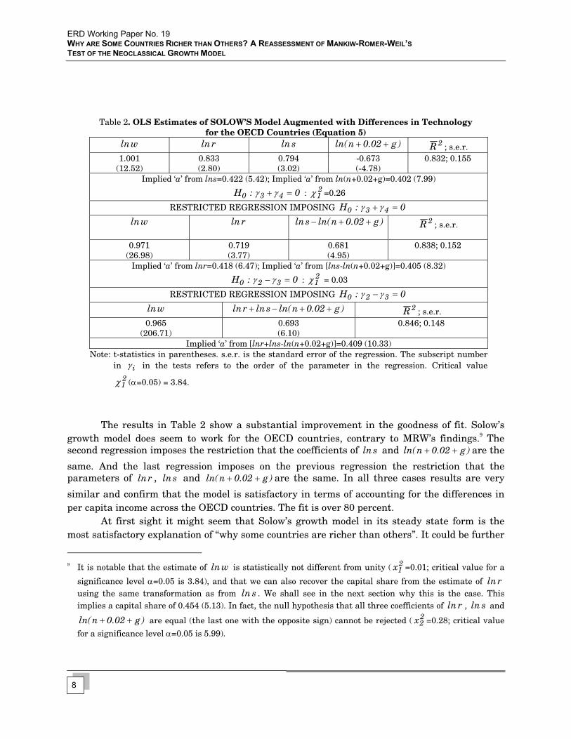
Table 1. OLS Estimates of MRW’s Specification of SOLOW’s Model

for the OECD Countries (Equation 3) Constant sln )05.0nln( + 2R ; s.e.r.

8.77 (3.51)

0.586 (1.36)

-0.605 (-0.71)

0.025; 0.37

Implied ‘a’ from lns = 0.369 (2.16); Implied ‘a’ from ln(n+0.05) = 0.377 (1.15)

0:H 320 =+ γγ : = 0 21χ

RESTRICTED REGRESSION IMPOSING 0:H 320 =+ γγ

Constant )05.0nln(sln +− 2R ; s.e.r. 8.82

(16.71) 0.591 (1.63)

0.073; 0.364

Implied ‘a’ from [ ln )05.0nln(s +− ] = 0.371 (2.59) Note: t-statistics in parentheses; s.e.r. is the standard error of the regression; ‘a’ is the capital share.

The subscript number in iγ in the tests refers to the order of the parameter in the regression.

The implied capital share ‘a’ is obtained as , where is the estimated

coefficient. Critical value (α=0.05) = 3.84.

)b1/(ba += b21χ

These results are consistent with those of MRW and thus will not be discussed further. Table 2 shows the second set of results, namely from the estimation of equation (5).8

7

8 The model is estimated with the constant term constrained to ln(2.024)=0.705. Hence, the dependent variable

is ln(Y/L)-0.705. The reason why we do this will become clear in the next section.


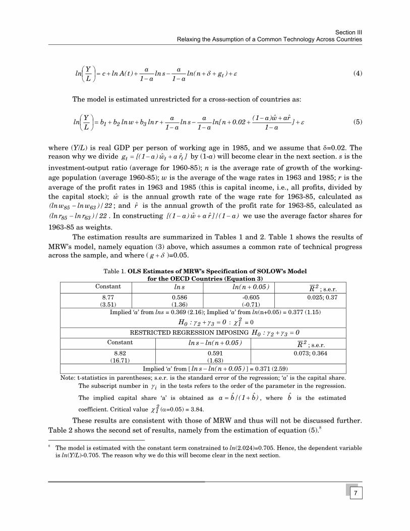
Table 2. OLS Estimates of SOLOW’S Model Augmented with Differences in Technology

for the OECD Countries (Equation 5) wln rln sln )g02.0nln( ++ 2R ; s.e.r.

1.001 (12.52)

0.833 (2.80)

0.794 (3.02)

-0.673 (-4.78)

0.832; 0.155

Implied ‘a’ from lns=0.422 (5.42); Implied ‘a’ from ln(n+0.02+g)=0.402 (7.99)

0:H 430 =+ γγ : =0.26 21χ

RESTRICTED REGRESSION IMPOSING 0:H 430 =+ γγ

wln rln )g02.0nln(sln ++−

2R ; s.e.r.

0.971 (26.98)

0.719 (3.77)

0.681 (4.95)

0.838; 0.152

Implied ‘a’ from lnr=0.418 (6.47); Implied ‘a’ from [lns-ln(n+0.02+g)]=0.405 (8.32)

0:H 320 =−γγ : = 0.03 21χ

RESTRICTED REGRESSION IMPOSING 0:H 320 =−γγ

wln )g02.0nln(slnrln ++−+ 2R ; s.e.r. 0.965

(206.71) 0.693 (6.10)

0.846; 0.148

Implied ‘a’ from [lnr+lns-ln(n+0.02+g)]=0.409 (10.33) Note: t-statistics in parentheses. s.e.r. is the standard error of the regression. The subscript number

in iγ in the tests refers to the order of the parameter in the regression. Critical value

(α=0.05) = 3.84. 21χ

The results in Table 2 show a substantial improvement in the goodness of fit. Solow’s

growth model does seem to work for the OECD countries, contrary to MRW’s findings.9 The second regression imposes the restriction that the coefficients of and are the

same. And the last regression imposes on the previous regression the restriction that the parameters of , and

sln )g02.0nln( ++

rln sln )g02.0nln( ++ are the same. In all three cases results are very

similar and confirm that the model is satisfactory in terms of accounting for the differences in per capita income across the OECD countries. The fit is over 80 percent.

At first sight it might seem that Solow’s growth model in its steady state form is the most satisfactory explanation of “why some countries are richer than others”. It could be further

9 It is notable that the estimate of is statistically not different from unity ( =0.01; critical value for a

significance level α=0.05 is 3.84), and that we can also recover the capital share from the estimate of ln using the same transformation as from . We shall see in the next section why this is the case. This implies a capital share of 0.454 (5.13). In fact, the null hypothesis that all three coefficients of , and

are equal (the last one with the opposite sign) cannot be rejected ( =0.28; critical value

for a significance level α=0.05 is 5.99).

wln 21x

rsln

rln sln

)g02.0nln( ++ 22x

8

Section IVToo Good to be True: The Tyranny of the Accounting Identity

argued that these results strongly justify MRW’s faith in Solow’s model. Countries are rich (poor) because they have high (low) investment rates, low (high) population growth rates, and high (low) levels of technology. See Jones (1998, 53) for a similar view.

On the other hand, paradoxically a suspicion arises. This is that perhaps the results are too good to be true because of all the theoretical problems associated with the concept of aggregate production function (Fisher 1993). Furthermore, it is surprising that only three variables (technology, employment, and capital), notwithstanding their likely serious measurement problems, so comprehensively explain the variation in per capita income.10

When Jones (1998, 54) plotted the predicted steady-state value of relative (with respect to the United States) income per capita against true relative income per capita, he found that virtually all his 104 countries fell on the 45-degree line, giving a very close fit (similar to the almost perfect fit given by the regression analysis), and concluded that “the Solow framework is extremely successful in helping us to understand the wide variation in the wealth of nations” (Jones 1998, 56).

In the next section it is shown why the data must, indeed, always give a near perfect fit to the estimated regression. This raises serious problems for the previous interpretations of Solow’s model. In this sense, we believe our arguments go beyond those of Brock and Durlauf (2001) in their criticisms of the empirical growth literature, namely, that it is difficult to know what variables to include in the analysis; and that the validity of a theory does not imply the falsity of another one, the assumption of parameter heterogeneity across countries, and the lack of attention to endogeneity problems.

IV. TOO GOOD TO BE TRUE: THE TYRANNY OF THE ACCOUNTING IDENTITY

In this section it is shown that the results in the last section can be regarded as merely a

statistical artifact. This is because the above results are totally determined by the income accounting identity that relates value added to the sum of the wage bill plus total profits.

The identity is given by:

ttttt KrLwY += (6)

where is real value added, is the real wage rate and is the ex-post real average profit

rate. This identity simply shows how total output is divided between wages and total profits (i.e., normal return to capital plus economic profits). Therefore, equation (6) does not follow from Euler’s theorem. The wage and profit rates need not be related to the (aggregate) marginal products which, in the light of the aggregation literature, most likely do not even exist (Fisher

tY tw tr

9

10 Srinivasan (1994, 1995) argues the data in the Summers and Heston database, the one used by most authors,

are of very poor quality since most of the data for the developing countries are constructed by extrapolation and interpolation.


1971a, 1971b).11 Furthermore, the aggregate production function itself is unlikely to be well defined and even to exist (Fisher 1969, 1993).12

The accounting identity in growth rates (assuming factor shares are constant) is given by:

tttttttt KaL)a1(KaL)a1(raw)a1(Y +−+=+−++−= φ (7)

where ttt raw)a1( +−=φ , is the labor share, and ttt Y/)Lw(a1 =− ttt Y/)Kr(a = is capital’s share. It will be noticed that the expression for tφ coincides what we called above the dual

measurement of productivity. However, if the aggregate production and cost functions do not exist (as opposed to the microeconomic relationships), the interpretation of tφ as a

measurement of technical progress becomes problematical.13 It is sufficient to note that equation (7) follows directly as a transformation of the accounting identity, equation (6), without any behavioral assumption (such as competitive markets). The only assumption is the constancy of the shares, which can occur for a number of reasons totally unrelated to the existence of an aggregate production function, such as when firms pursue a constant markup pricing policy.

Integrating equation (7) and taking antilogarithms gives:

at

a1t0

at

a1t

at

a1t0t K L )t(B BK L rw BY −−− == (8)

11 It is common to argue that if capital and labor are paid their marginal products, constant returns to scale

implies wL+rK=F(K,AL). r is defined as ( ) K/AL,KF ∂∂ and w as ( ) L/AL,KF ∂∂ (Romer 1996, 35). This is

misleading, and even wrong. In the words of Fisher: “If aggregate capital does not exist, then of course one cannot believe in the marginal productivity of aggregate capital” (Fisher 1971b, 405; italics in the original). The conditions to generate an aggregator of labor are also extremely restrictive, so the same comment applies to the (aggregate) marginal product of labor. The previous result follows from Euler’s theorem which, while correct as a mathematical proposition, conflicts with the aggregation problem in economics. If the aggregates K and L cannot be constructed because of the aggregation problems, then the function F(K, AL) does not exist, and it follows that wL+rK=F(K,AL) has no meaning. Therefore, the notion of estimates of returns to scale at the aggregate level becomes problematic, to say the least. The identity VA=wL+rK will nevertheless always hold. In the words of Samuelson: “No one can stop us from labeling this last vector [residually computed profit returns to “property” or to the nonlabor factor] as (RCj), as J.B. Clark’s model would permit–even though we have no warrant for believing that noncompetitive industries have a common profit rate R and use leets capital (Cj) in proportion to the (Pjqj – WjLj) elements!” (Samuelson 1979, 932).

12 In this sense we strongly disagree with Romer (1996, 8) who claims that the critical assumption of the aggregate production function in Solow’s model is that it has constant returns in capital and labor. The crucial assumption in the authors’ opinion is that the aggregate production function exists. Felipe and Fisher (2003) summarize the most important results of the aggregation literature and discuss why economists continue using a tool without sound theoretical underpinning.

13 It must be clear that the idea of total factor productivity (in its primal and dual forms) at the aggregate is linked to the notions of aggregate production and cost functions (Nadiri 1970). Without the latter there is no reason why the so-called residual tφ in the income accounting identity must be a measure of productivity.

Notice, for example, that the weights (the factor shares) appear in this derivation without invoking the first-order conditions. All this follows from the supposed link between the identity, the aggregate production function, and Euler’s theorem.

10


where .14 Equation (8) is not a production function. It is simply the income

identity, equation (6), rewritten under the assumption that factor shares are constant. Also note that the factor shares appear without invoking the marginal productivity conditions.15 We elaborate upon this below.

at

a1t r w)t(B −=

The definition of the increase in the capital stock is:

ttt KIK δ−≡∆ (9)

where I is gross investment and δ is the constant rate of depreciation. It is a definition because this is the way the capital stock is calculated in practice, using net investment and the perpetual inventory method. From this it follows that:

δδ −=−==∆

t

t

t

tt

t

tKsY

KI

KKK (10)

where s is the constant investment-output ratio.

Let us make our second assumption that the capital-output ratio does not change over

time, so that . While this is a condition for steady state growth in the neoclassical

schema, it is also one of Kaldor’s stylized facts, unrelated to neoclassical theory (Barro and Sala-i-Martin 1995, 5). Using this assumption, equation (7) becomes

tt KY =

0LK La1

K KaL)a1(KY 'tttt

ttttttt =−−⇒+

−=⇒+−+== φφφ (11)

14 is referred to in the neoclassical literature as the dual measure of productivity. It can be

called anything one wants to, but certainly what we have done here (to rewrite an identity) is very different from the standard derivation of the dual in neoclassical economics. What we have done is correct, but tautological.

at

a1t r w)t(B −=

15 This implies that if the assumption of constant shares is correct in the data set in question, the regression

must yield 21tt0t K L )t(B BY αα= a11 −=α and a2 =α and a perfect fit (compare with equation [8]).

This assumption, in practice, is correct for most data sets. Therefore, why do researchers sometimes obtain “increasing returns to scale”? The answer is that B(t) is incorrectly proxied, often through a linear time trend, i.e., B(t)=exp(λ t). If this approximation is incorrect (as most often is), it will induce a bias in the estimates of

1α and 2α (maybe even negative values; see Lucas 1970 and Tatom 1980). But this does not undermine our

argument. The correct proxy for B(t) will yield the best possible regression and hence, will take us back to the identity.

11


where a1

raw)a1(a1

ttt't −

+−=

−=

φφ . Substituting from (10) into (11) and denoting

yields:

tK nLt =

0nKsY '

tt

t =−−− φδ (12)

Denoting , the level of output per effective unit of labor, and

the stock of capital per effective unit of labor allows us to rewrite equation

(12) as

)L)t(B/Y(y ttt =

)L)t(B/K(k ttt =

0nksy '

tt

t =−−− φδ (13)

or,

tt

t yn

sk

φδ ++= (14)

and equation (8) as

a

t0t ]k )t(B[ By = (15)

By substituting (14) into (15) we obtain

a1a

't

a1a

0tn

s )t(B Cy

−−

++=

φδ (16)

where . From here it follows that: )a1/(1

00 )B(C −=

)nln(a1

asln

a1a

)t(Blna1

1 c

LY

ln 't

t

t φδ ++−

−−

+−

+=

(17)

where , and substituting for B(t) and gives: )Cln(c 0= '

tφ

]a1

raw)a1(nln[

a1a

slna1

a]rlnawln)a1[(

a11

cLY

ln tttt

t

t−

+−++

−−

−++−

−+=

δ (18)

or,

]a1

raw)a1(nln[

a1a

slna1

arln

a1a

wln1.0cLY

ln tttt

t

t−

+−++

−−

−+

−++=

δ (19)

12


The question that arises at this point is: how is equation (19) to be interpreted?16 This is

the same dilemma we posed at the end of last section. It is obvious that equation (19) resembles equation (3) above, and that it is identical with equation (5). Equation (3) is the form derived by MRW to test Solow’s model. The difference is that the first expression in equation (19), i.e., the logarithm of the wage and profit rates, appears subsumed into the constant term in (3), and that the last term of equation (19), i.e., the weighted average of the growth rates of the wage and profit rates was assumed to be constant by MRW. Therefore, it could be argued that equation (19) is a more general specification that can be used to test Solow's model. This is because, under this interpretation, we have started with the cost function and, by assuming constant shares, have posited that the underlying production function is in fact a Cobb-Douglas. A constant capital-output ratio has also been assumed, implying equation (19) refers to steady-state growth. The approach set out above is more general than that of MRW because international differences in the rate of technological progress have been allowed for. Under this neoclassical interpretation, it could be argued that the results of estimating this model provide a striking confirmation of the Solow model. This is because all the estimated coefficients are not significantly different from the values that are expected a priori if all countries fulfilled the usual neoclassical assumptions (i.e., existence of the neoclassical aggregate production function and the marginal productivity conditions) and were at their steady state.

There is, however, a more plausible alternative interpretation of equation (19). This is that all we have done is to transform the income accounting identity, equation (6), into another identity, provided the two assumptions used, namely, constant factor shares, and constant capital-output ratio, are empirically correct.17 Recall our arguments above about equations (6) and (8): they are identities. What is important to notice is that equation (6) and the two assumptions made are equally compatible with the absence of a well-behaved aggregate production function, there is no requirement that factors be paid their marginal products, about the state of competition, or about steady-state. Indeed, if the assumptions are (exactly) correct, econometric estimation of equation (19) must yield a perfect fit, and simply because of the underlying identity (and not for any other reason), we should expect the estimates of the profit rate, saving rate, and that of the sum of the growth rate of the labor force plus depreciation plus “technical progress” to give a ballpark figure of , or 2/3 (with the appropriate sign) for 0.4. The estimate of the wage rate should equal unity.

)a1/(ab −=

≅a

16 Since we are not dealing with a true behavioral model but with an identity we can recover the value of the

constant term. From it follows that at

a1t

at

a1t0t K L rw BY −−=

a1aa1

ta

t

t0

)a1(a

1

]Y)a1[()aY(

YB

−− −=

−= , since factor shares are constant.

17 The assumptions of constancy of the shares and of the capital-output ratio refer across countries.

13


But can all this be interpreted to be a test, in the sense of providing verification (strictly speaking, nonrefutation) of Solow’s model? The answer is clearly “no” because, as we have noted, the estimates are compatible with the assumption of a no well-defined aggregate production function. Moreover, an of unity should be a clear sign of suspicion. 2R

The argument implies is that if factor shares and the capital-output ratio are constant, equation (19) will always yield a high fit (with data for any sample of countries) and with the corresponding parameters. Furthermore, if ttt r aw )a1(g +−= and are

constant, then equation (19) becomes MRW’s equation (3), and it will indeed give highly significant and plausible estimates.

aa10 )t(r )t(w B)t(A −=

As indicated above, the two assumptions used are quite general. The hypothesis of a constant capital-output ratio is one of Kaldor’s stylized facts. It is a very general proposition.18 Regarding the assumption of constant shares, it could be asked whether it implies a Cobb-Douglas production function. It is standard to argue that the reason why factor shares appear to be more or less constant is that the underlying technology of the economy is Cobb-Douglas (Mankiw 1995, 288). The answer, however, is that this is not necessarily the case. In his seminal simulation work, Fisher (1971a) simulated a series of micro-economies with Cobb-Douglas production functions. He aggregated them deliberately violating the conditions for successful aggregation. He found, to his surprise, that when factor shares were constant the aggregate Cobb-Douglas worked very well. This led him to conclude that the (standard) view that constancy of the labor share is due to the presence of an aggregate Cobb-Douglas production function is erroneous. In fact, he concluded, the argument runs the other way around, that is, the aggregate Cobb-Douglas works well because labor’s share is roughly constant. Thus, what the argument says is that the Cobb-Douglas will work as long factor shares are constant, even though the true underlying technology might be fixed coefficients.19 Factor shares will be constant, for example, if firms follow a constant mark-up on wages pricing policy (Lee 1999) with any underlying technology at the plant level.20

The conclusion is that if the two assumptions used above are empirically correct, the national income accounts imply that an equation like (19) exists, and we will always find that there is a positive relationship between the savings rate and income per capita, and a negative relationship between population growth and income per capita.

18 And certainly the British economist would be rather displeased to find out that this stylized fact is

interpreted in terms of an aggregate production function, a notion that for many years he fought against. 19 In the neoclassical model, factor shares are constant in the steady state for any production function. Mankiw

(1995, 288) indicates that factor shares may be roughly constant in the US data merely because the US economy has not recently been far from its steady state.

20 See also Nelson and Winter (1982), who create a non-neoclassical economy that leads to constant factor shares and where a Cobb-Douglas yields good results.

14


But the important question, we insist, is whether this approach this can in any way be interpreted as a test of Solow’s model. The answer is, again, no. If the estimated coefficients are identical to those predicted by equation (19), it could be because the model satisfies all the Solovian assumptions, but the estimated coefficients are equally compatible with none of Solow’s assumptions being valid. The data cannot discriminate between the two hypotheses and all one can say is that the assumptions of constant shares and a constant capital-output ratio have not been refuted.21

The case perhaps more difficult to gauge is the one when there is not a perfect fit to the data, like in MRW (and virtually all applications). In fact, with data taken from the national accounts we will never obtain a perfect fit. The reason is simply that neither factor shares nor the capital-output ratio are exactly constant. Does this then imply a rejection of Solow’s model? We continue arguing it does not. All this means is that either factor shares or the capital-output ratio is not constant. The first can be taken under a neoclassical interpretation as a rejection that the underlying production function is a Cobb-Douglas. However, we can always find a better approximation to the identity (and which will resemble another production function) that allows factor shares to vary, and this could be (erroneously) interpreted as a production function. The second does refute the proposition that growth is in steady-state, but the results convey no more information than if a direct test of whether the capital-output ratio is constant were undertaken.

Moreover, given our arguments, statistical estimation of equation (19) is not needed. One simply has to check whether the two assumptions above are empirically correct. For most countries, the assumption that factor shares are constant is correct. Indeed, factor shares vary very slowly and within a narrow range. This is true in our data set. Factor shares increased slightly in the 25-year period considered but display very little variation across countries in both initial and terminal years. So, it all comes down to checking whether the capital-output ratio is constant. Here again we observe a similar pattern: capital-output ratios increased in time in all countries but the standard deviations in both initial and terminal years were small and identical in both periods. We conclude that, overall, equation (19) has to work well in terms of fit and yield estimates close to the hypothesized results.

A related important issue is that estimation of equation (19) does not require instrumental variable methods, as MRW (1992, 411) suggest, because the equation is fundamentally an identity. The error term here, if any, derives from an incorrect approximation to the income accounting identity. There is no endogeneity problem in the standard sense.

21 One may be also tempted to argue that the problem is similar to that of observational equivalence, in this

case between equations (19) and (5) (or equation (3) if technology levels and growth rates are constant across countries). However, for this argument to be correct, one would have to deal with two models that have the same implications about observable phenomena under all circumstances. Here, however, we do not have two alternative theories that generate the same distribution of observations. One of them is the alleged theory (Solow’s), but the other one is just an identity. Therefore, this is not an identification problem the strict sense. Placing a priori restrictions on Solow’s model will never identify an identity. On the observational equivalence problem in macroeconomics see Backhouse and Salanti (2000).

15


Certainly, wage rate, profit rate, employment and capital are endogenous variables, but nobody would argue that estimation of equation (6), an identity, requires instrumental variables, since there is no error term. If equation (19) is a perfect approximation to equation (6), the argument remains. It is true, however, that if equation (19) is not a perfect approximation to equation (6), the estimation method will matter. It may be possible that instrumental variable estimation, for example, could yield, under these circumstances, estimates closer to the theoretical values. But this is a minor issue once the whole argument is appreciated.

The implications of this argument are far reaching. It is not possible to test the predictions of Solow’s growth model, as it is known a priori what the estimates will be. Equation (19) is little more than a tautology. Moreover, it now becomes clear why Jones’ (1998) procedure gives such results. By calculating the level of technology from the supposed production function as A=Y/F(K,L) (see equation [8]), all Jones (1998) and Hall and Jones (1999) did was to calculate the weighted average of the wage and profit rates. This is their measure of productivity. In the neoclassical theory this is referred to as the dual or price based measure of productivity. However, it arises as a tautology, without invoking any theory.22

Jones (1998) substituted A=Y/F(K,L) into the steady-state solution (i.e., an expression comparable to equation [14] above, which follows from the identity too).23 In other words, all that was achieved was a return to the underlying identity.24 Hall and Jones (1999, 94) asked: “What do the measured differences in productivity across countries actually reflect?” They argued, following Solow (1957), that they measure differences in the quality of human capital, on-the-job training, or vintage effects (Romer [1996, 25] defines A in a similar way). And as a corollary they argue that a theory of productivity differences is needed.25 While they are correct in focusing on the determinants of productivity differences such as disparities in social infrastructure, their procedure for calculating technology is problematic since ‘A’ is, by

22 In that framework, the profit rate is computed independently, and thus the accounting identity need not hold,

hence the relationship with the production function and Euler’s theorem. As we have argued above, however, the identity must hold always.

23 As indicated above, this method was first used by Solow (1957). Solow used the production function to calculate the level of technology, which was then used to “deflate” the production function in order to remove the effect of technical change. In terms of equation (8), Solow constructed the series , where

y=Y/L. Then he regressed on . It is little wonder that he found a fit of over 0.99.

)t(B/yq tt =

tq ttt L/Kk =24 Jones (1998, equation 3.1) and Hall and Jones (1999, equation 1) used a production function with human

capital (H). It is easy to show that “technology”, calculated as A=Y/F(K,H), where (u is defined as the average educational attainment of the labor force (i.e., years of schooling) and ψ is the return to schooling (i.e., percentage by which each year of schooling increases a worker’s wage), can be computed as

from the accounting identity (equation [8] above). Jones indicates that “estimates of A

computed this way are the residuals from growth accounting: they incorporate any differences in production not factored in through the inputs” (Jones 1998, 55; italics original).

L eH uψ=

u)a1/(att e/rw ψ−

25 This idea had been previously expressed by Prescott (1998).

16


definition, a weighted average of the wage and profit rates.26 It is one thing to argue that we need a theory of the components of equation (7) (that is, the factor shares, growth rates of the wage and profit rates, and the growth rates of capital and labor), and of how productivity and growth feed each other, in order to explain differences in growth. It is quite another thing to estimate equation (7) as Y (or a transformation of it), to test whether

the estimated coefficients are equal to the factor shares, and take this is as a test of a growth

theory.

t4t3t2t1t KbLbrbwbˆ +++=

ib

What is the result of further augmenting Solow’s model in the sense of including additional variables, such as human capital? If the variables used in these regressions are statistically significant, it must be because they serve as a proxy for the weighted average of the wage and profit rates. Consequently, they reduce, to some extent, the degree of omitted variable bias. As noted above, Knowles and Owen (1995) and Nonneman and Vanhoudt (1996) extended the model by introducing health capital and the average annual ratio of gross domestic expenditure on research and development to nominal GDP, respectively. The correlations between the logarithm of this variable and the logarithms of wages and profit rates are 0.811 and –0.768, respectively. It is not surprising that the addition of this variable to the MRW specification improved the fit of the model as they found a “good” proxy for B(t), although the savings rate, the proxy for human capital, and the growth rate of employment plus technology and depreciation, were statistically insignificant. This is because Nonneman and Vanhoudt were still using , and thus was poorly approximated (same for the modification of

Knowles and Owen 1995).

)05.0nln( + 'tφ

Islam (1995), on the other hand, used panel estimation and heterogeneous intercepts. The use of individual country dummies also helps to approximate better the identity. And finally, Temple (1998) correctly pointed out that the MRW specification lacks robustness. The problem, however, is not that the model is flawed because its goodness of fit varies substantially with the sample of countries. Even the specification given by equation (19), derived directly from the identity, may conceivably not give a close fit. It all depends on whether or not the assumptions used (viz. constant factor shares and a constant capital-output ratio), are approximately correct. It would be possible to find a sample of countries where these do not hold and thus there would be a poor fit to the identity. This would not, however, affect the theoretical argument concerning the problems posed by the underlying identity for the interpretation of the parameters of the model.

We close this section by quoting Solow (1994) in reference to this research program (see also the first footnote above): “The temptation of wishful thinking hovers over the interpretation of these cross-section studies. It should be countered by cheerful skepticism. The introduction of a wide range of explanatory variables has the advantage of offering partial

17

26 Hall and Jones (1999) conclude that differences in institutions and government policies (social infrastructure

in general) cause differences in “productivity”. This is a rather non-neoclassical and interesting explanation of the wage and profit rates.


shelter from the bias due to omitted variables. But this protection is paid for. As the range of explanation broadens, it becomes harder and harder to believe in an underlying structural, reversible relation that amounts to more than a sly way of saying that Japan grew rapidly and the United Kingdom slowly during this period” (Solow 1994, 51).27

V. THE CONVERGENCE REGRESSION AND THE SPEED OF CONVERGENCE It is necessary to consider the implications of this argument for estimates of the speed of

convergence given by the MRW specification. One of the main points MRW stressed in their paper was that Solow’s growth model predicts conditional, not absolute, convergence. Convergence works through lags in the diffusion of knowledge (income difference might tend to shrink as poorer countries gain access to best-practice technology) and through differential rates of return on capital (capital flows to the countries with a lower capital-labor ratio, where the rate of return is higher).

The speed of convergence, denoted by λ, measures how quickly a deviation from the steady state growth rate is corrected over time. In other words, it indicates the percentage of the deviation from steady state that is eliminated each year. A rapid rate of convergence implies that economies are close to their steady states. When MRW tested for conditional convergence they found that indeed it occurs, but the rate implied by Solow’s model is much faster than the rate the convergence regressions indicate. A number of studies, including MRW’s, have found evidence of conditional convergence at a rate of about 2 percent per year. That is, each country moves 2 percent closer to its own steady state each year (Mankiw 1995, 285). This implies that the economy moves halfway to steady state in about 35 years. On the other hand, it can be shown that the speed of convergence according to Solow’s model equals )a1( )gn( −++= δλ

(Barro and Sala-i-Martin 1995, 36-38; Mankiw 1995, 285). Using the averages in our data set (we assume δ=0.02), λ= (0.01+0.02+0.021)*0.768 = 0.0391, or 3.91 percent per year, almost twice the rate that most studies estimate.

The convergence regression is derived by taking an approximation around the steady state (Mankiw 1995). Empirically, λ is estimated through a regression of the difference in

27 Romer (2001) has very strong words against this research program from a methodological point of view. In

essence, he argues that what this program has done is to advocate a narrow methodology based on model testing and on using strong theoretical priors with a view to restricting attention to a very small subset of all possible models. “Then show that one of the models from within this narrow set fits the data and, if possible, show that there are other models that do not. Having tested and rejected some models so that the exercise looks like it has some statistical power, accept the model that fits the data as a “good model” ” (Romer 2001, 226). Romer is correct in his assessment that MRW never considered alternative models. For example, the finding of a negative coefficient for the initial income variable is interpreted, in the context of the neoclassical model, as evidence of diminishing returns to capital. But, as Romer argues, this finding could also be interpreted as implying that the technology of the country that starts at a lower level of development is lower and it grows faster as better technology diffuses there. Romer claims that MRW’s approach does not advance science and refers to it as refers to it as a dead end.

18

Section VThe Convergence Regression and the Speed of Convergence

income per capita between the final and initial periods on the same regressors as previously used (i.e., savings rate and the sum of the growth rate of employment, depreciation rate, and technology), plus the level of income per capita in the initial period. The coefficient of the initial income variable (τ) is a function of the speed of convergence, namely, (MRW,

1992, 423). This equation is:

)e1( tλτ −−−=

ετλλ +++−

−−−

−+=− −−0

tt00t yln)05.0nln(

a1a

)e1(slna1

a)e1(b)ylny(ln (20)

where and are the levels of income per worker in 1985 and 1960, respectively. ty 0y

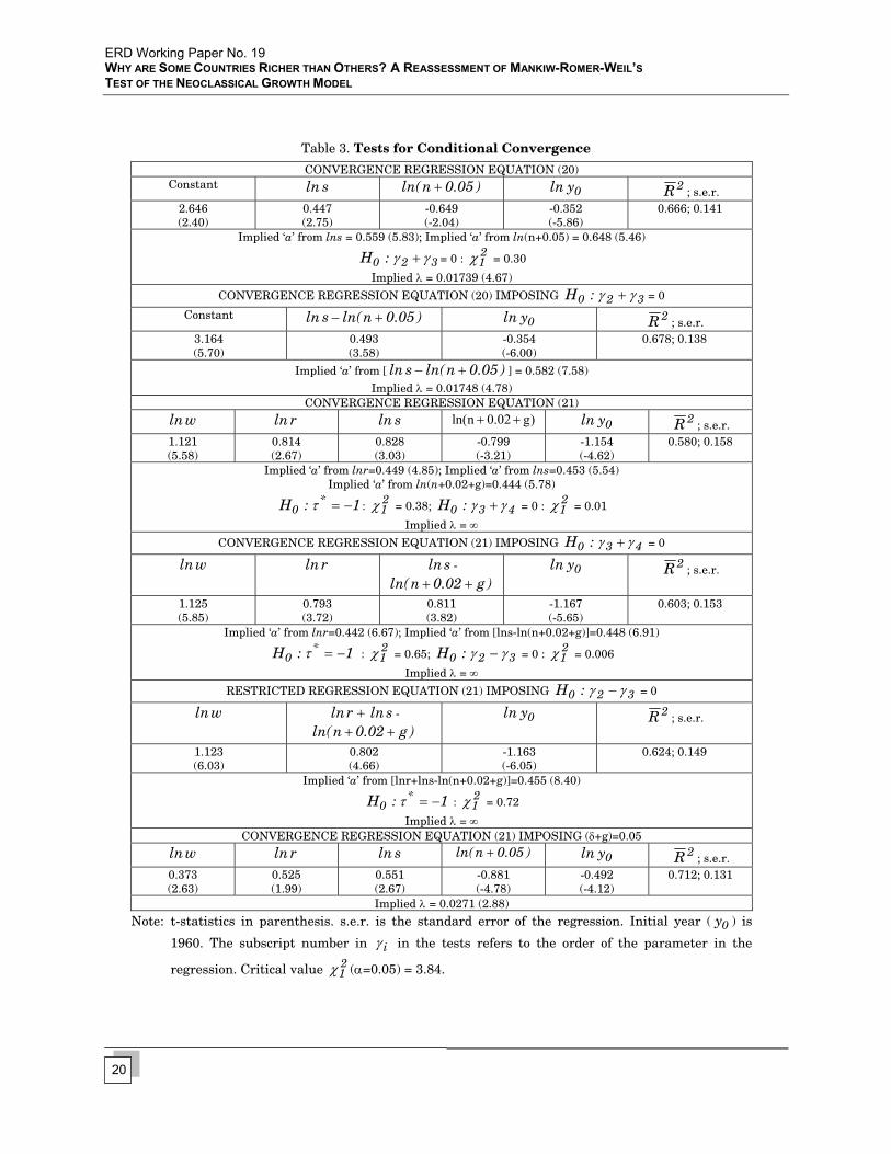
Estimation results of equation (20) are displayed in the upper part of Table 3 (the first two regressions, where the coefficients are estimated unrestricted and restricted, respectively). The results are close to those of MRW (1992, Table IV), with a very similar speed of convergence, slightly below to 2 percent a year.28

What do the arguments in Section 4 imply for the convergence regression and the speed of convergence? In terms of equation (19) above, this specification can derived by subtracting the logarithm of income per capita in the initial period from both sides of the equation. This yields:

−−

+−

++=− slna1

arln

a1a

wln1.0 c)ylny(ln tt0t

0*tt yln]

a1raw)a1(

nln[a1

aτδ +

−+−

++−

− (21)

Equation (21) indicates that the parameter of has to be = -1 (i.e., the estimate

obtained is minus unity). Our argument indicates that since equation (19) is essentially an identity, subtraction of on both sides implies that the estimate of will be minus one.

The third, fourth, and fifth regressions in Table 3 show the OLS estimates of equation (21).29

0yln *τ

ln0yln 0y

19

28 The speed of convergence is derived from the last coefficient, that is, . Once λ is determined,

implied capital share is obtained from the other coefficients. )e1( tλτ −−−=

29 Equation (21) is also estimated with the restricted constant.


Table 3. Tests for Conditional Convergence

CONVERGENCE REGRESSION EQUATION (20) Constant sln )05.0nln( + 0yln 2R ; s.e.r.

2.646 (2.40)

0.447 (2.75)

-0.649 (-2.04)

-0.352 (-5.86)

0.666; 0.141

Implied ‘a’ from lns = 0.559 (5.83); Implied ‘a’ from ln(n+0.05) = 0.648 (5.46)

320 :H γγ + = 0 : = 0.30 21χ

Implied λ = 0.01739 (4.67)

CONVERGENCE REGRESSION EQUATION (20) IMPOSING 320 :H γγ + = 0

Constant )05.0nln(sln +− 0yln 2R ; s.e.r. 3.164 (5.70)

0.493 (3.58)

-0.354 (-6.00)

0.678; 0.138

Implied ‘a’ from [ )05.0nln(sln +− ] = 0.582 (7.58) Implied λ = 0.01748 (4.78)

CONVERGENCE REGRESSION EQUATION (21)

wln rln sln )g02.0nln( ++ 0yln 2R ; s.e.r. 1.121 (5.58)

0.814 (2.67)

0.828 (3.03)

-0.799 (-3.21)

-1.154 (-4.62)

0.580; 0.158

Implied ‘a’ from lnr=0.449 (4.85); Implied ‘a’ from lns=0.453 (5.54) Implied ‘a’ from ln(n+0.02+g)=0.444 (5.78)

1:H *0 −=τ : = 0.38; 2

1χ 430 :H γγ + = 0 : = 0.01 21χ

Implied λ = ∞

CONVERGENCE REGRESSION EQUATION (21) IMPOSING 430 :H γγ + = 0

wln rln sln02.0

-

)gnln( ++ 0yln 2R ; s.e.r.

1.125 (5.85)

0.793 (3.72)

0.811 (3.82)

-1.167 (-5.65)

0.603; 0.153

Implied ‘a’ from lnr=0.442 (6.67); Implied ‘a’ from [lns-ln(n+0.02+g)]=0.448 (6.91)

1:H *0 −=τ : = 0.65; 2

1χ 320 :H γγ − = 0 : = 0.006 21χ

Implied λ = ∞

RESTRICTED REGRESSION EQUATION (21) IMPOSING 320 :H γγ − = 0

wln +rln.0n

sln02

-

)gln( ++ 0yln 2R ; s.e.r.

1.123 (6.03)

0.802 (4.66)

-1.163 (-6.05)

0.624; 0.149

Implied ‘a’ from [lnr+lns-ln(n+0.02+g)]=0.455 (8.40)

1:H *0 −=τ : = 0.72 2

1χImplied λ = ∞

CONVERGENCE REGRESSION EQUATION (21) IMPOSING (δ+g)=0.05

wln rln sln )05.0nln( + 0yln 2R ; s.e.r. 0.373 (2.63)

0.525 (1.99)

0.551 (2.67)

-0.881 (-4.78)

-0.492 (-4.12)

0.712; 0.131

Implied λ = 0.0271 (2.88)

Note: t-statistics in parenthesis. s.e.r. is the standard error of the regression. Initial year ( ) is

1960. The subscript number in 0y

iγ in the tests refers to the order of the parameter in the

regression. Critical value (α=0.05) = 3.84. 21χ

20

Section VThe Convergence Regression and the Speed of Convergence

These results provide a very different picture of the convergence discussion. The findings for are as predicted, and the rest of the parameters continue being very well estimated in terms of size and sign (and the restrictions on the parameters continue to not being rejected).30 If this equation were to be interpreted as being the neoclassical growth model, the results imply

, or λ = ∞ (under the null hypothesis that ). The neoclassical

interpretation would be presumably that the speed of convergence is infinite and all countries are growing at or near their steady state.31 But, as we have seen, with differences in “technical progress” allowed for, the identity will always give this result. The only reason why the conventional estimates are greater than minus unity is due to the assumption imposed on the model of a spatially constant rate of technical change and a constant level of technology.32

*τ

(−= 1)e1 t* −=− −λτ 1* −=τ

As one better approximates the identity by including other variables in the regression (compare Tables IV and V in MRW 1992, or the augmentations by Nonneman and Vandhout 1996) or by including heterogeneous intercepts (Islam 1995) and allowing the growth rates of technology to differ (Lee et al. 1997), the speed of convergence increases because variations in B(t) and are better captured. Durlauf and Johnson (1995, 370 and 375, Tables II and V)

found higher rates of convergence in the regressions for each subsample than in the single regime, but rejected the hypothesis of convergence among the high-output economies. On the other hand, Temple (1998, 369, Table 3) did not find much higher rates of convergence, except in the lowest quartile (9.2 percent a year). The exchange between Lee et al. (1998) and Islam (1998) concerned differences in the size of λ as a consequence of the different estimation methods and assumptions about what is allowed to vary. Lee et al. (1998) report regressions where the mean speed convergence increases to 0.23 (when the restriction that g is the same across countries is relaxed) and to 0.29 (with heterogeneity in λ and in g). Islam’s (1998, 325) intuition in his exchange with Lee et al. (1998) was correct: “Clearly, a different estimation method is not the main reason for this substantial increase.” Maddala and Wu’s (2000)

'tφ

30 Notice that the coefficients of and sln )05.0nln( + are multiplied by in equation (20), and they are not

in equation (21). However, since the estimate of must be unity, it does not affect the result.

*τ*τ

31 We believe that his result implies that if countries are at their steady state growth rate, the speed of

convergence is undefined. See equation (13) in MRW, i.e., what occurs if . )t(ylnyln * =32 Islam (1995, equation 11) argues that a better way to estimate the rate of convergence is through an equation

that incorporates transitional behavior. He derives an equation with on the left-hand side (as opposed

to the difference between last and initial periods) and with on the right hand side (and the same other

regressors, i.e., and ln . He acknowledges (Islam 1995, 11) that his regression has the same

omitted-variable bias problem as MRW’s equation, due to an improper account of A0. In this case, and from the point of view of the accounting identity, the estimate of has to be zero, leading to the same

conclusions about the speed of convergence as with the MRW regression. As Islam’s approximation to the identity is substantially worse than that provided by equation (21), it seems that he is estimating a true behavioral equation. Lee et al. (1998, 321) indicate that the estimate of tends to unity in the

probability limit. And Quah (1996) shows that the 2 percent convergence rate observed is a statistical artifact, the product of “unit root econometrics in disguise.”

tyln

0

0ylnsln ( 05.0n + )

yln

0yln

21


estimation procedure allowed them to calculate individual convergence rates for the OECD countries. Their estimates range from 1.27 percent per year for Switzerland to 10.32 percent per year for West Germany, with an average for the 17 OECD European countries of 4.68 percent per year. And when they separate the sample into different periods, the average convergence rate increases to 19.7 percent per year for 1950-1960.

As has been shown, as the restrictions on B(t) and (i.e., that they are common) are

relaxed (i.e., that they are the same across countries), the convergence regression estimated approximates equation (21) better, τ tends to unity and λ increases. But this must be true irrespective of the sample size, the number of countries (in the context of panel estimation) and the estimator used. Although the exchange between Lee et al. (1998) and Islam (1998) about the meaning of convergence when one permits heterogeneity in growth rates provides some useful insights (most notably that the very concept of convergence becomes problematical), it is not appreciated that the underlying problem is more fundamental, namely, that no matter what method is used to estimate this regression, the results will be conditioned by the presence of the underlying accounting identity. Technical fixes do not solve the problem. The last regression in Table 3 shows equation (21) estimated with a common (g in MRW). The results are very

similar to those of Islam (1995, 1141, Table I). The biases and other econometric issues discussed by Islam (1995, 1998); Lee et al. (1998); and Maddala and Wu (2000) are not fundamentally econometric problems. The whole argument rests on how close the regression used approximates the income accounting identity.

'tφ

'tφ

VI. CONCLUSIONS: WHAT IS LEFT OF SOLOW’S GROWTH MODEL? Why are some countries richer than others? Is the neoclassical growth model, based on

an aggregate production function, a useful theory of economic growth? This paper has evaluated whether the predictions of Solow’s growth modelnamely, that the higher the rate of saving, the richer the country; and the higher the rate of population growth, the poorer the countrycan be tested and potentially refuted.

We have used MRW’s specification of Solow’s model and shown that a form identical to that used by MRW can be derived by simply transforming the income accounting identity that relates output to the sum of the total wage bill plus total profits. To do this only requires the assumptions that factor shares and the capital-output ratio are constant. This has allowed us to question that indeed Solow’s growth model can be tested in the sense of it being capable of refutation.

It has been argued that the key to understanding the results discussed in the literature lies in the assumption of a common level of technology and rate of technical progress across countries. Although this assumption has been discussed in the literature, authors have missed the important point that all that is being estimated is an approximation to an accounting identity. From this point of view, the assumption of a common rate of technological progress

22

Section VIConclusions: What is Left of Solow’s Growth Model?

amounts to treating the weighted average of the wage and profit rates that appears in the accounting identity as a constant across countries. The form derived from the accounting identity explicitly incorporating differences in growth of the weighted average of the wage and profit rates and using only two assumptions, is so close to the identity itself that it explains most of the variation in income per capita in the OECD countries. MRW’ regression, on the other hand, explained only one percent. This form, or a good approximation to it, guarantees a high statistical fit, and where the implicit values of the output elasticities are very close to the respective factor shares. The estimate of the coefficient of the savings rate must be positive and that of the sum of employment and technology growth rates must be negative. All this is solely the result of the accounting identity. It has been argued that MRW’s equation imposes on the identity the empirically incorrect assumptions that the weighted average of the wage and profit rates and the weighted average of the growth rates of the wage and profit rates are constant across countries. The fact that this gives a less than perfect statistical fit may give the impression that a behavioral regression, rather than an identity is actually being estimated.

The conditional convergence equation discussed in the literature is also affected by our arguments. It has been shown that once the weighted average of the wage and profit rates is properly introduced, the “identity” predicts that the speed of convergence, under neoclassical assumptions, must be infinite. Certainly this is a most implausible result.

The conclusion that has to be drawn is that the predictions of Solow’s growth model cannot be tested econometrically because they cannot be refuted. In view of the above findings, it is difficult to find an optimistic note on which to close. This framework does not help answer the central question of why some countries are richer than others. The implications of the paper, therefore, go far beyond a mere critique or a proposal for improvement in the estimation and testing of the neoclassical growth model. The problem discussed is far more fundamental than that of the necessity for a further augmentation of Solow’s model, or the use of more appropriate econometric techniques.

From the policy perspective (Kenny and Williams 2000, Rashid 2000), the argument implies that we cannot measure the impact of standard growth policies, e.g., the effect on an increase in the savings rate on income per capita. However, our arguments should not be taken as implying that a country’s income level is not, in some sense, related to savings and investment, population growth, and technology, any more than that the production of an individual commodity is not related to the volume of inputs used. The arguments should not be misconstrued either as a claim that any regression explaining income per capita is futile because, one way or another, the right-hand side variables (e.g., countries’ latitude) are proxying the right-hand side variables of the income accounting identity. The same applies to the convergence literature, that is, studying whether historically countries have tended to converge is an important issue (the notion of sigma-convergence is not effected by our arguments). And a regression of growth rates on initial income (and perhaps other variables) certainly says something. As Easterly and Levine (2001) indicate “The coefficient on initial income does not necessarily capture only neoclassical transitional dynamics. In technology

23


diffusion models, initial income may proxy for the initial gap in TFP between economies. In these models, therefore, catch-up can be in TFP as well as in traditional factors of production” (Easterly and Levine 2001, p.209).33 What has to be inferred is that the neoclassical growth model, as formulated in MRW’s specification and derived from an aggregate production function, cannot be the place to start any discussion about growth, development and convergence.

In the authors’ opinion, the above calls for a serious reconsideration of the neoclassical growth model and its explanatory power of differences in income per capita. If we are going to continue using this framework in order to think about questions of growth, we need a different procedure and methodology to test the predictions of the neoclassical model. Given that the whole framework depends on the existence of the aggregate production function, the feasibility of this option seems problematical. We see two options open. First, perhaps the discussion of economic growth should be formulated in terms other than the neoclassical production function, perhaps along the lines of evolutionary growth models (Nelson and Winter 1982). Secondly, the accounting identity, equation (6) could be used as a reference framework to expand on the proposal to develop a theory of TFP differences, as advocated by Prescott (1998) and Easterly and Levine (2001) (although certainly outside the neoclassical model and the aggregate production function framework). As equations (6) and (7) show, the rate of TFP growth is always, by virtue of the identity, a weighted average of the wage and profit rates. This, it must be stressed, is true always. Therefore, any theory explaining TFP (or its growth rate) must be implicitly a theory of this weighted average. We hope that realizing that the mystery lies in this weighted average will shed light.

Felipe and Fisher (2003) conclude their survey by arguing that “macroeconomists should pause before continuing to do applied work with no sound foundation and dedicate some time to studying other approaches to value, distribution, employment, growth, technical progress, etc., in order to understand which questions can legitimately be posed to the empirical aggregate data.” It is not possible to rely on the instrumentalist argument that as all models necessarily involve abstraction because they are stories, the fact that the neoclassical growth model can give good statistical fits means that aggregation problems can be ignored as empirically unimportant. It has been shown precisely why these models if correctly specified must always give good statistical fits. A model that cannot be potentially refuted empirically is not a productive metaphor.

33 The technology gap approach, for example, posits that the rate of economic growth of a country is positively

influenced by the rate of growth in the technological level of the country. Other important variables in this paradigm are the catch up process and the country’s ability to mobilize resources for transforming social, institutional, and economic structures. See Fagerberg (1987).

24

References

REFERENCES Backhouse, R. E., and A. Salanti, 2000. “Introduction.” In R. E. Backhouse and A. Salanti, eds.,

Macroeconomics and the Real World. Oxford and New York: Oxford University Press. Barro, R. J., and X. Sala-i-Martin, 1995. Economic Growth. New York: McGraw Hill. Bernanke, B. S., and R. S. Gürkaynak, 2001. Is Growth Exogenous? Taking Mankiw, Romer,

and Weil Seriously. NBER Working Paper 8365, National Bureau of Economic Research, Massachusetts.

Bliss, C., 1999. “Galton’s Fallacy and Economic Convergence.” Oxford Economic Papers 51:4-14. Brock, W. A., and S. N. Durlauf, 2001. “What Have We Learned from a Decade of Empirical

Research on Growth? Growth Empirics and Reality.” World Bank Economic Review 15(2):229-72.

Cannon, E. S., and N. W. Duck, 2000. “Galton’s Fallacy and Economic Convergence.” Oxford Economic Papers 52:415-9.

Durlauf, S., 2000. “Econometric Analysis and the Study of Economic Growth: A Sceptical Perspective.” In R. E. Backhouse and A. Salanti, eds., Macroeconomics and the Real World. Oxford and New York: Oxford University Press.

Durlauf, S. N., and P. A. Johnson, 1995. “Multiple Regimes and Cross-Country Growth Behavior.” Journal of Applied Econometrics 10:365-84.

Durlauf, S., and D. Quah, 1999. “The New Empirics of Economic Growth.” In J. Taylor and M. Woodford, eds., Handbook of Macroeconomics. Amsterdam: North Holland.

Easterly, W., and R. Levine, 2001. “It’s Not Factor Accumulation: Stylized Facts and Growth Models.” World Bank Economic Review 15(2):177-219.

Fagerberg, J., 1987. “A Technology Gap Approach to why Growth Rates Differ.” Research Policy 16:87-99.

Felipe, J., and F. M. Fisher, 2003. “Aggregation in Production Functions: What Applied Economists Should Know.” Metroeconomica. Forthcoming.

Fisher, F. M., 1969. “The Existence of Aggregate Production Functions.” Econometrica 37(4, October):553-77.

, 1971a. “Aggregate Production Functions and the Explanation of Wages: A Simulation Experiment.” The Review of Economics and Statistics LIII(4, November):305-25.

, 1971b. “Reply.” Econometrica 39(2, March):405. , 1993. Aggregation. Aggregate Production Functions and Related Topics. Cambridge, MA:

The MIT Press. Hall, R. E., and C. I. Jones, 1999. “Why Do Some Countries Produce so much more Output than

Others?” Quarterly Journal of Economics 114(February):83-116. Islam, N., 1995. “Growth Empirics: A Panel Data Approach.” Quarterly Journal of Economics

90:1127-70. , 1998. “Growth Empirics: A Panel Data ApproachA Reply.” Quarterly Journal of

Economics 113(1, February):325-9.

25


, 1999. “International Comparisons of Total Factor Productivity: A Review.” Review of Income and Wealth 45(4, December):493-518.

Jones, C. I., 1997. “Comment.” In B. S. Bernanke and J. Rotemberg, eds., NBER Macroeconomics Annual 1997. Cambridge: The MIT Press.

, 1998. Introduction to Economic Growth. New York: W. W. Norton & Co., Inc. Jorgenson, D. W., 1995. Productivity: Post-war U.S. Economic Growth. Cambridge: MIT Press. Kenny, C., and D. Williams, 2000. “What Do We Know about Economic Growth? Or, Why Don’t

We Know Very Much?” World Development 29(1):1-22. Klenow, P., and A. Rodriguez-Clare, 1997. “The Neoclassical Revival in Growth Economics: Has

It Gone Too Far?” NBER Macroeconomics Annual 12:73-103. Knowles, S., and P. Dorian Owen, 1995. “Health Capital and Cross-Country Variation in Income

per Capita in the Mankiw-Romer-Weil Model.” Economics Letters 48:99-106. Lee, F. S. 1998. Post-Keynesian Price Theory. Cambridge: Cambridge University Press. Lee, K., M. Hashem Pesararan, and R. Smith, 1997. “Growth and Convergence in a Multi-

Country Empirical Stochastic Solow Model.” Journal of Applied Econometrics XII:357-92.

1998. “Growth Empirics: A Panel Data Approach –A Comment.” Quarterly Journal of Economics 113(1, February):319-23.

Lucas, R., 1970. “Capacity, Overtime, and Empirical Production Functions.” American Economic Review Papers and Proceedings 60(2, May):23-7.

Maddala, G. S., and S. Wu, 2000. “Cross-Country Growth Regressions: Problems of Heterogeneity and Interpretation.” Applied Economics 32:635-42.

Mankiw, G., 1995. “The Growth of Nations” Brookings Papers on Economic Activity 1(September):275-325.

, 1997. “Comment.” In B. S. Bernanke and J. Rotemberg, eds., NBER Macroeconomics Annual 1997. Cambridge: The MIT Press.

Mankiw, G., D. Romer, and D. N. Weil. 1992: “A Contribution to the Empirics of Economic Growth.” Quarterly Journal of Economics 107(2, May):407-37.

Nadiri, I. M., 1970. “Some Approaches to the Theory and Measurement of Total Factor Productivity: A Survey.” Journal of Economic Literature VIII(December):1137-77.

Nelson, R., and S. G. Winter. 1982. An Evolutionary Theory of Economic Change. Cambridge, MA: Harvard University Press.

Nonneman, W., and P. Vanhoudt. 1996. “A Further Augmentation of the Solow Model and the Empirics of Economic Growth for OECD Countries.” Quarterly Journal of Economics 111:943-53.

Pack, H., 1994. “Endogenous Growth Theory: Intellectual Appeal and Empirical Shortcomings.” Journal of Economic Perspectives 8(1, Winter):55-72.

Parente, S., and E. C. Prescott, 1994. “Barriers to Technology Adoption and Development.” Journal of Political Economy 102(2):298-321.

26

References

Prescott, E. C., 1998. “Needed: A Theory of Total Factor Productivity.” International Economic Review.39(3, August):525-52.

Quah, D., 1993a. “Galton’s Fallacy and Tests of the Convergence Hypothesis.” Scandinavian Journal of Economics 95(4):427-43.

, 1993b. “Empirical Cross-Section Dynamics in Economic Growth.” European Economic Review 37:426-34.

, 1996. “Empirics for Economic Growth and Convergence. European Economic Review 40:1353-75.

Rashid, S., 2000. Economic Policy for Growth. Economic Development is Human Development. Boston: Kluwer Academic Press.

Romer, D., 1996. Advanced Macroeconomics. New York: McGraw Hill. Romer, P., 2001. “Comment on “It’s Not Factor Accumulation: Stylized Facts and Growth

Models.” World Bank Economic Review 15(2):225-7. Sala-i-Martin, X., 2001. “What Have We Learned from a Decade of Empirical Research on

Growth? Comment on “Growth Empirics and Reality” by William A. Brock and Steven N. Durlauf. ” World Bank Economic Review 15(2):277-82.

Samuelson, P. A., 1979. “Paul Douglas’s Measurement of Production Functions and Marginal Productivities.” Journal of Political Economy 87:923-39.

Simon, H., 1979. “Rational Decision Making in Business Organizations.” American Economic Review 69(4, September):493-513.

Solow, R., 1956. “A Contribution to the Theory of Economic Growth.” Quarterly Journal of Economics 70:65-94.

, 1957. “Technical Change and the Aggregate Production Function.” Review of Economics and Statistics 39:312-20.

, 1988. “Growth Theory and After.” American Economic Review 78(3):307-17. , 1994. “Perspectives on Growth Theory.” Journal of Economic Perspectives8(1,

Winter):45-54. , 2001. “What Have We Learned from a Decade of Empirical Research on Growth?

Applying Growth Theory across Countries.” World Bank Economic Review 15(2):283-8. Srinivasan, T. N., 1994. “Data Base for Development Analysis: An Overview.” Journal of

Development Analysis 44:3-27. , 1995. “Long-run Growth Theories and Empirics: Anything New? In T. Ito and A. C.

Krueger, eds., Growth Theories in Light of the East Asian Experience. Chicago: University of Chicago Press.

Tatom, J. A. 1980. “The ‘Problem’ of Procyclical Real Wages and Productivity.” Journal of Political Economy 88(2):385-94.

Temple, J., 1998. “Robustness Tests of the Augmented Solow Model.” Journal of Applied Econometrics 13:361-75.

, 1999. “The New Growth Evidence.” Journal of Economic Literature XXXVII(March):112-56.

27

28

PUBLICATIONS FROM THEECONOMICS AND RESEARCH DEPARTMENT

ERD WORKING PAPER SERIES (WPS)(Published in-house; Available through ADB Office of External Relations; Free of Charge)

No. 1 Capitalizing on Globalization—Barry Eichengreen, January 2002

No. 2 Policy-based Lending and Poverty Reduction:An Overview of Processes, Assessmentand Options—Richard Bolt and Manabu Fujimura

January 2002No. 3 The Automotive Supply Chain: Global Trends

and Asian Perspectives—Francisco Veloso and Rajiv Kumar

January 2002No. 4 International Competitiveness of Asian Firms:

An Analytical Framework—Rajiv Kumar and Doren Chadee

February 2002No. 5 The International Competitiveness of Asian

Economies in the Apparel Commodity Chain—Gary Gereffi

February 2002No. 6 Monetary and Financial Cooperation in East

Asia—The Chiang Mai Initiative and Beyond—Pradumna B. Rana

February 2002No. 7 Probing Beneath Cross-national Averages: Poverty,

Inequality, and Growth in the Philippines—Arsenio M. Balisacan and Ernesto M. Pernia

March 2002No. 8 Poverty, Growth, and Inequality in Thailand

—Anil B. DeolalikarApril 2002

No. 9 Microfinance in Northeast Thailand: Who Benefitsand How Much?—Brett E. Coleman

April 2002No. 10 PovertyReduction and the Role of Institutions in

Developing Asia—Anil B. Deolalikar, Alex B. Brilliantes, Jr.,

Raghav Gaiha, Ernesto M. Pernia, Mary Raceliswith the assistance of Marita Concepcion Castro-

ERD TECHNICAL NOTE SERIES (TNS)(Published in-house; Available through ADB Office of External Relations; Free of Charge)

No. 1 Contingency Calculations for EnvironmentalImpacts with Unknown Monetary Values—David Dole February 2002

No. 2 Integrating Risk into ADB’s Economic Analysisof Projects—Nigel Rayner, Anneli Lagman-Martin,

and Keith Ward June 2002

Guevara, Liza L. Lim, Pilipinas F. QuisingMay 2002

No. 11 The European Social Model: Lessons forDeveloping Countries—Assar Lindbeck

May 2002No. 12 Costs and Benefits of a Common Currency for

ASEAN—Srinivasa Madhur

May 2002No. 13 Monetary Cooperation in East Asia: A Survey

—Raul FabellaMay 2002

No. 14 Toward A Political Economy Approachto Prolicy-based Lending—George Abonyi

May 2002No. 15 A Framework for Establishing Priorities in a

Country Poverty Reduction Strategy—Ron Duncan and Steve Pollard

June 2002No. 16 The Role of Infrastructure in Land-use Dynamics

and Rice Production in Viet Nam’s Mekong RiverDelta—Christopher Edmonds

July 2002No. 17 Effect of Decentralization Strategy on

Macroeconomic Stability in Thailand—Kanokpan Lao-Araya

August 2002No. 18 Poverty and Patterns of Growth

—Rana Hasan and M. G. QuibriaAugust 2002

No. 19 Why are Some Countries Richer than Others?A Reassessment of Mankiw-Romer-Weil’s Test ofthe Neoclassical Growth Model—Jesus Felipe and John McCombie

August 2002

No. 3 Measuring Willingness to Pay for Electricity—Peter Choynowski July 2002

No. 4 Economic Issues in the Design and Analysis of aWastewater Treatment Project—David Dole

July 2002

29

MONOGRAPH SERIES(Published in-house; Available through ADB Office of External Relations; Free of charge)

EDRC REPORT SERIES (ER)

ERD POLICY BRIEF SERIES (PBS)(Published in-house; Available through ADB Office of External Relations; Free of charge)

No. 1 Is Growth Good Enough for the Poor?—Ernesto M. Pernia, October 2001

No. 2 India’s Economic ReformsWhat Has Been Accomplished?What Remains to Be Done?—Arvind Panagariya, November 2001

No. 3 Unequal Benefits of Growth in Viet Nam—Indu Bhushan, Erik Bloom, and Nguyen MinhThang, January 2002

No. 4 Is Volatility Built into Today’s World Economy?—J. Malcolm Dowling and J.P. Verbiest,February 2002

No. 5 What Else Besides Growth Matters to PovertyReduction? Philippines—Arsenio M. Balisacan and Ernesto M. Pernia,February 2002

No. 6 Achieving the Twin Objectives of Efficiency andEquity: Contracting Health Services in Cambodia—Indu Bhushan, Sheryl Keller, and BradSchwartz,March 2002

No. 7 Causes of the 1997 Asian Financial Crisis: WhatCan an Early Warning System Model Tell Us?—Juzhong Zhuang and Malcolm Dowling,June 2002

No. 8 The Role of Preferential Trading Arrangementsin Asia—Christopher Edmonds and Jean-Pierre Verbiest,July 2002

No. 9 The Doha Round: A Development Perspective—Jean-Pierre Verbiest, Jeffrey Liang, and LeaSumulong, July 2002

No. 1 ASEAN and the Asian Development Bank—Seiji Naya, April 1982

No. 2 Development Issues for the Developing Eastand Southeast Asian Countriesand International Cooperation—Seiji Naya and Graham Abbott, April 1982

No. 3 Aid, Savings, and Growth in the Asian Region—J. Malcolm Dowling and Ulrich Hiemenz,

April 1982No. 4 Development-oriented Foreign Investment

and the Role of ADB—Kiyoshi Kojima, April 1982

No. 5 The Multilateral Development Banksand the International Economy’s MissingPublic Sector—John Lewis, June 1982

No. 6 Notes on External Debt of DMCs—Evelyn Go, July 1982

No. 7 Grant Element in Bank Loans—Dal Hyun Kim, July 1982

No. 8 Shadow Exchange Rates and StandardConversion Factors in Project Evaluation—Peter Warr, September 1982

No. 9 Small and Medium-Scale ManufacturingEstablishments in ASEAN Countries:Perspectives and Policy Issues—Mathias Bruch and Ulrich Hiemenz,

January 1983No. 10 A Note on the Third Ministerial Meeting of GATT

—Jungsoo Lee, January 1983No. 11 Macroeconomic Forecasts for the Republic

of China, Hong Kong, and Republic of Korea—J.M. Dowling, January 1983

No. 12 ASEAN: Economic Situation and Prospects—Seiji Naya, March 1983

No. 13 The Future Prospects for the DevelopingCountries of Asia—Seiji Naya, March 1983

No. 14 Energy and Structural Change in the Asia-Pacific Region, Summary of the Thirteenth

Pacific Trade and Development Conference—Seiji Naya, March 1983

No. 15 A Survey of Empirical Studies on Demandfor Electricity with Special Emphasis on PriceElasticity of Demand—Wisarn Pupphavesa, June 1983

No. 16 Determinants of Paddy Production in Indonesia:1972-1981–A Simultaneous Equation ModelApproach—T.K. Jayaraman, June 1983

No. 17 The Philippine Economy: EconomicForecasts for 1983 and 1984—J.M. Dowling, E. Go, and C.N. Castillo,

June 1983No. 18 Economic Forecast for Indonesia

—J.M. Dowling, H.Y. Kim, Y.K. Wang,and C.N. Castillo, June 1983

No. 19 Relative External Debt Situation of AsianDeveloping Countries: An Applicationof Ranking Method—Jungsoo Lee, June 1983

No. 20 New Evidence on Yields, Fertilizer Application,and Prices in Asian Rice Production—William James and Teresita Ramirez, July 1983

No. 21 Inflationary Effects of Exchange RateChanges in Nine Asian LDCs—Pradumna B. Rana and J. Malcolm Dowling, Jr., December 1983

No. 22 Effects of External Shocks on the Balanceof Payments, Policy Responses, and DebtProblems of Asian Developing Countries—Seiji Naya, December 1983

No. 23 Changing Trade Patterns and Policy Issues:The Prospects for East and Southeast AsianDeveloping Countries—Seiji Naya and Ulrich Hiemenz, February 1984

No. 24 Small-Scale Industries in Asian EconomicDevelopment: Problems and Prospects—Seiji Naya, February 1984

No. 25 A Study on the External Debt Indicators

30

Applying Logit Analysis—Jungsoo Lee and Clarita Barretto, February 1984

No. 26 Alternatives to Institutional Credit Programsin the Agricultural Sector of Low-IncomeCountries—Jennifer Sour, March 1984

No. 27 Economic Scene in Asia and Its Special Features—Kedar N. Kohli, November 1984

No. 28 The Effect of Terms of Trade Changes on theBalance of Payments and Real NationalIncome of Asian Developing Countries—Jungsoo Lee and Lutgarda Labios, January 1985

No. 29 Cause and Effect in the World Sugar Market:Some Empirical Findings 1951-1982—Yoshihiro Iwasaki, February 1985

No. 30 Sources of Balance of Payments Problemin the 1970s: The Asian Experience—Pradumna Rana, February 1985

No. 31 India’s Manufactured Exports: An Analysisof Supply Sectors—Ifzal Ali, February 1985

No. 32 Meeting Basic Human Needs in AsianDeveloping Countries—Jungsoo Lee and Emma Banaria, March 1985

No. 33 The Impact of Foreign Capital Inflowon Investment and Economic Growthin Developing Asia—Evelyn Go, May 1985

No. 34 The Climate for Energy Developmentin the Pacific and Asian Region:Priorities and Perspectives—V.V. Desai, April 1986

No. 35 Impact of Appreciation of the Yen onDeveloping Member Countries of the Bank—Jungsoo Lee, Pradumna Rana, and Ifzal Ali,

May 1986No. 36 Smuggling and Domestic Economic Policies

in Developing Countries—A.H.M.N. Chowdhury, October 1986

No. 37 Public Investment Criteria: Economic InternalRate of Return and Equalizing Discount Rate—Ifzal Ali, November 1986

No. 38 Review of the Theory of Neoclassical PoliticalEconomy: An Application to Trade Policies—M.G. Quibria, December 1986

No. 39 Factors Influencing the Choice of Location:Local and Foreign Firms in the Philippines—E.M. Pernia and A.N. Herrin, February 1987

No. 40 A Demographic Perspective on DevelopingAsia and Its Relevance to the Bank—E.M. Pernia, May 1987

No. 41 Emerging Issues in Asia and Social CostBenefit Analysis—I. Ali, September 1988

No. 42 Shifting Revealed Comparative Advantage:Experiences of Asian and Pacific DevelopingCountries—P.B. Rana, November 1988

No. 43 Agricultural Price Policy in Asia:Issues and Areas of Reforms—I. Ali, November 1988

No. 44 Service Trade and Asian Developing Economies—M.G. Quibria, October 1989

No. 45 A Review of the Economic Analysis of PowerProjects in Asia and Identification of Areasof Improvement—I. Ali, November 1989

No. 46 Growth Perspective and Challenges for Asia:Areas for Policy Review and Research—I. Ali, November 1989

No. 47 An Approach to Estimating the PovertyAlleviation Impact of an Agricultural Project—I. Ali, January 1990

No. 48 Economic Growth Performance of Indonesia,the Philippines, and Thailand:The Human Resource Dimension—E.M. Pernia, January 1990

No. 49 Foreign Exchange and Fiscal Impact of a Project:A Methodological Framework for Estimation—I. Ali, February 1990

No. 50 Public Investment Criteria: Financialand Economic Internal Rates of Return—I. Ali, April 1990

No. 51 Evaluation of Water Supply Projects:An Economic Framework—Arlene M. Tadle, June 1990

No. 52 Interrelationship Between Shadow Prices, ProjectInvestment, and Policy Reforms:An Analytical Framework—I. Ali, November 1990

No. 53 Issues in Assessing the Impact of Projectand Sector Adjustment Lending—I. Ali, December 1990

No. 54 Some Aspects of Urbanizationand the Environment in Southeast Asia—Ernesto M. Pernia, January 1991

No. 55 Financial Sector and EconomicDevelopment: A Survey—Jungsoo Lee, September 1991

No. 56 A Framework for Justifying Bank-AssistedEducation Projects in Asia: A Reviewof the Socioeconomic Analysisand Identification of Areas of Improvement—Etienne Van De Walle, February 1992

No. 57 Medium-term Growth-StabilizationRelationship in Asian Developing Countriesand Some Policy Considerations—Yun-Hwan Kim, February 1993

No. 58 Urbanization, Population Distribution,and Economic Development in Asia—Ernesto M. Pernia, February 1993

No. 59 The Need for Fiscal Consolidation in Nepal:The Results of a Simulation—Filippo di Mauro and Ronald Antonio Butiong,

July 1993No. 60 A Computable General Equilibrium Model

of Nepal—Timothy Buehrer and Filippo di Mauro,

October 1993No. 61 The Role of Government in Export Expansion

in the Republic of Korea: A Revisit—Yun-Hwan Kim, February 1994

No. 62 Rural Reforms, Structural Change,and Agricultural Growth inthe People’s Republic of China—Bo Lin, August 1994

No. 63 Incentives and Regulation for Pollution Abatementwith an Application to Waste Water Treatment—Sudipto Mundle, U. Shankar,and Shekhar Mehta, October 1995

No. 64 Saving Transitions in Southeast Asia—Frank Harrigan, February 1996

No. 65 Total Factor Productivity Growth in East Asia:A Critical Survey—Jesus Felipe, September 1997

No. 66 Foreign Direct Investment in Pakistan:Policy Issues and Operational Implications—Ashfaque H. Khan and Yun-Hwan Kim,

July 1999No. 67 Fiscal Policy, Income Distribution and Growth

—Sailesh K. Jha, November 1999

31

No. 1 International Reserves:Factors Determining Needs and Adequacy—Evelyn Go, May 1981

No. 2 Domestic Savings in Selected DevelopingAsian Countries—Basil Moore, assisted by

A.H.M. Nuruddin Chowdhury, September 1981No. 3 Changes in Consumption, Imports and Exports

of Oil Since 1973: A Preliminary Survey ofthe Developing Member Countriesof the Asian Development Bank—Dal Hyun Kim and Graham Abbott,

September 1981No. 4 By-Passed Areas, Regional Inequalities,

and Development Policies in SelectedSoutheast Asian Countries—William James, October 1981

No. 5 Asian Agriculture and Economic Development—William James, March 1982

No. 6 Inflation in Developing Member Countries:An Analysis of Recent Trends—A.H.M. Nuruddin Chowdhury and

J. Malcolm Dowling, March 1982No. 7 Industrial Growth and Employment in

Developing Asian Countries: Issues andPerspectives for the Coming Decade—Ulrich Hiemenz, March 1982

No. 8 Petrodollar Recycling 1973-1980.Part 1: Regional Adjustments andthe World Economy—Burnham Campbell, April 1982

No. 9 Developing Asia: The Importanceof Domestic Policies—Economics Office Staff under the direction

of Seiji Naya, May 1982No. 10 Financial Development and Household

Savings: Issues in Domestic ResourceMobilization in Asian Developing Countries—Wan-Soon Kim, July 1982

No. 11 Industrial Development: Role of SpecializedFinancial Institutions—Kedar N. Kohli, August 1982

No. 12 Petrodollar Recycling 1973-1980.Part II: Debt Problems and an Evaluationof Suggested Remedies—Burnham Campbell, September 1982

No. 13 Credit Rationing, Rural Savings, and FinancialPolicy in Developing Countries—William James, September 1982

No. 14 Small and Medium-Scale ManufacturingEstablishments in ASEAN Countries:Perspectives and Policy Issues—Mathias Bruch and Ulrich Hiemenz, March 1983

No. 15 Income Distribution and EconomicGrowth in Developing Asian Countries—J. Malcolm Dowling and David Soo, March 1983

No. 16 Long-Run Debt-Servicing Capacity ofAsian Developing Countries: An Applicationof Critical Interest Rate Approach—Jungsoo Lee, June 1983

No. 17 External Shocks, Energy Policy,and Macroeconomic Performance of AsianDeveloping Countries: A Policy Analysis—William James, July 1983

No. 18 The Impact of the Current Exchange RateSystem on Trade and Inflation of SelectedDeveloping Member Countries—Pradumna Rana, September 1983

No. 19 Asian Agriculture in Transition: Key Policy Issues—William James, September 1983

No. 20 The Transition to an Industrial Economy

ECONOMIC STAFF PAPERS (ES)

in Monsoon Asia—Harry T. Oshima, October 1983

No. 21 The Significance of Off-Farm Employmentand Incomes in Post-War East Asian Growth—Harry T. Oshima, January 1984

No. 22 Income Distribution and Poverty in SelectedAsian Countries—John Malcolm Dowling, Jr., November 1984

No. 23 ASEAN Economies and ASEAN EconomicCooperation—Narongchai Akrasanee, November 1984

No. 24 Economic Analysis of Power Projects—Nitin Desai, January 1985

No. 25 Exports and Economic Growth in the Asian Region—Pradumna Rana, February 1985

No. 26 Patterns of External Financing of DMCs—E. Go, May 1985

No. 27 Industrial Technology Developmentthe Republic of Korea—S.Y. Lo, July 1985

No. 28 Risk Analysis and Project Selection:A Review of Practical Issues—J.K. Johnson, August 1985

No. 29 Rice in Indonesia: Price Policy and ComparativeAdvantage—I. Ali, January 1986

No. 30 Effects of Foreign Capital Inflowson Developing Countries of Asia—Jungsoo Lee, Pradumna B. Rana,

and Yoshihiro Iwasaki, April 1986No. 31 Economic Analysis of the Environmental

Impacts of Development Projects—John A. Dixon et al., EAPI,

East-West Center, August 1986No. 32 Science and Technology for Development:

Role of the Bank—Kedar N. Kohli and Ifzal Ali, November 1986

No. 33 Satellite Remote Sensing in the Asianand Pacific Region—Mohan Sundara Rajan, December 1986

No. 34 Changes in the Export Patterns of Asian andPacific Developing Countries: An EmpiricalOverview—Pradumna B. Rana, January 1987

No. 35 Agricultural Price Policy in Nepal—Gerald C. Nelson, March 1987

No. 36 Implications of Falling Primary CommodityPrices for Agricultural Strategy in the Philippines—Ifzal Ali, September 1987

No. 37 Determining Irrigation Charges: A Framework—Prabhakar B. Ghate, October 1987

No. 38 The Role of Fertilizer Subsidies in AgriculturalProduction: A Review of Select Issues—M.G. Quibria, October 1987

No. 39 Domestic Adjustment to External Shocksin Developing Asia—Jungsoo Lee, October 1987

No. 40 Improving Domestic Resource Mobilizationthrough Financial Development: Indonesia—Philip Erquiaga, November 1987

No. 41 Recent Trends and Issues on Foreign DirectInvestment in Asian and Pacific DevelopingCountries—P.B. Rana, March 1988

No. 42 Manufactured Exports from the Philippines:A Sector Profile and an Agenda for Reform—I. Ali, September 1988

No. 43 A Framework for Evaluating the EconomicBenefits of Power Projects—I. Ali, August 1989

No. 44 Promotion of Manufactured Exports in Pakistan

32

—Jungsoo Lee and Yoshihiro Iwasaki,September 1989

No. 45 Education and Labor Markets in Indonesia:A Sector Survey—Ernesto M. Pernia and David N. Wilson,

September 1989No. 46 Industrial Technology Capabilities

and Policies in Selected ADCs—Hiroshi Kakazu, June 1990

No. 47 Designing Strategies and Policiesfor Managing Structural Change in Asia—Ifzal Ali, June 1990

No. 48 The Completion of the Single European Commu-nity Market in 1992: A Tentative Assessment ofits Impact on Asian Developing Countries—J.P. Verbiest and Min Tang, June 1991

No. 49 Economic Analysis of Investment in PowerSystems—Ifzal Ali, June 1991

No. 50 External Finance and the Role of MultilateralFinancial Institutions in South Asia:Changing Patterns, Prospects, and Challenges—Jungsoo Lee, November 1991

No. 51 The Gender and Poverty Nexus: Issues andPolicies—M.G. Quibria, November 1993

No. 52 The Role of the State in Economic Development:Theory, the East Asian Experience,and the Malaysian Case

—Jason Brown, December 1993No. 53 The Economic Benefits of Potable Water Supply

Projects to Households in Developing Countries—Dale Whittington and Venkateswarlu Swarna,

January 1994No. 54 Growth Triangles: Conceptual Issues

and Operational Problems—Min Tang and Myo Thant, February 1994

No. 55 The Emerging Global Trading Environmentand Developing Asia—Arvind Panagariya, M.G. Quibria,

and Narhari Rao, July 1996No. 56 Aspects of Urban Water and Sanitation in

the Context of Rapid Urbanization inDeveloping Asia—Ernesto M. Pernia and Stella LF. Alabastro,

September 1997No. 57 Challenges for Asia’s Trade and Environment

—Douglas H. Brooks, January 1998No. 58 Economic Analysis of Health Sector Projects-

A Review of Issues, Methods, and Approaches—Ramesh Adhikari, Paul Gertler, and

Anneli Lagman, March 1999No. 59 The Asian Crisis: An Alternate View

—Rajiv Kumar and Bibek Debroy, July 1999No. 60 Social Consequences of the Financial Crisis in

Asia—James C. Knowles, Ernesto M. Pernia, and

Mary Racelis, November 1999

No. 1 Poverty in the People’s Republic of China:Recent Developments and Scopefor Bank Assistance—K.H. Moinuddin, November 1992

No. 2 The Eastern Islands of Indonesia: An Overviewof Development Needs and Potential—Brien K. Parkinson, January 1993

No. 3 Rural Institutional Finance in Bangladeshand Nepal: Review and Agenda for Reforms—A.H.M.N. Chowdhury and Marcelia C. Garcia,

November 1993No. 4 Fiscal Deficits and Current Account Imbalances

of the South Pacific Countries:A Case Study of Vanuatu—T.K. Jayaraman, December 1993

No. 5 Reforms in the Transitional Economies of Asia—Pradumna B. Rana, December 1993

No. 6 Environmental Challenges in the People’s Republicof China and Scope for Bank Assistance—Elisabetta Capannelli and Omkar L. Shrestha,

December 1993No. 7 Sustainable Development Environment

and Poverty Nexus—K.F. Jalal, December 1993

No. 8 Intermediate Services and EconomicDevelopment: The Malaysian Example—Sutanu Behuria and Rahul Khullar, May 1994

No. 9 Interest Rate Deregulation: A Brief Surveyof the Policy Issues and the Asian Experience—Carlos J. Glower, July 1994

No. 10 Some Aspects of Land Administrationin Indonesia: Implications for Bank Operations—Sutanu Behuria, July 1994

No. 11 Demographic and Socioeconomic Determinantsof Contraceptive Use among Urban Women inthe Melanesian Countries in the South Pacific:A Case Study of Port Vila Town in Vanuatu—T.K. Jayaraman, February 1995

No. 12 Managing Development throughInstitution Building— Hilton L. Root, October 1995

No. 13 Growth, Structural Change, and OptimalPoverty Interventions—Shiladitya Chatterjee, November 1995

No. 14 Private Investment and MacroeconomicEnvironment in the South Pacific IslandCountries: A Cross-Country Analysis—T.K. Jayaraman, October 1996

No. 15 The Rural-Urban Transition in Viet Nam:Some Selected Issues—Sudipto Mundle and Brian Van Arkadie,

October 1997No. 16 A New Approach to Setting the Future

Transport Agenda—Roger Allport, Geoff Key, and Charles Melhuish

June 1998No. 17 Adjustment and Distribution:

The Indian Experience—Sudipto Mundle and V.B. Tulasidhar, June 1998

No. 18 Tax Reforms in Viet Nam: A Selective Analysis—Sudipto Mundle, December 1998

No. 19 Surges and Volatility of Private Capital Flows toAsian Developing Countries: Implicationsfor Multilateral Development Banks—Pradumna B. Rana, December 1998

No. 20 The Millennium Round and the Asian Economies:An Introduction—Dilip K. Das, October 1999

No. 21 Occupational Segregation and the GenderEarnings Gap—Joseph E. Zveglich, Jr. and Yana van der MeulenRodgers, December 1999

No. 22 Information Technology: Next Locomotive ofGrowth?—Dilip K. Das, June 2000

OCCASIONAL PAPERS (OP)

33

1. Improving Domestic Resource Mobilization ThroughFinancial Development: Overview September 1985

2. Improving Domestic Resource Mobilization ThroughFinancial Development: Bangladesh July 1986

3. Improving Domestic Resource Mobilization ThroughFinancial Development: Sri Lanka April 1987

4. Improving Domestic Resource Mobilization ThroughFinancial Development: India December 1987

5. Financing Public Sector Development Expenditurein Selected Countries: Overview January 1988

6. Study of Selected Industries: A Brief ReportApril 1988

7. Financing Public Sector Development Expenditurein Selected Countries: Bangladesh June 1988

8. Financing Public Sector Development Expenditurein Selected Countries: India June 1988

9. Financing Public Sector Development Expenditurein Selected Countries: Indonesia June 1988

10. Financing Public Sector Development Expenditurein Selected Countries: Nepal June 1988

11. Financing Public Sector Development Expenditurein Selected Countries: Pakistan June 1988

12. Financing Public Sector Development Expenditurein Selected Countries: Philippines June 1988

13. Financing Public Sector Development Expenditurein Selected Countries: Thailand June 1988

14. Towards Regional Cooperation in South Asia:ADB/EWC Symposium on Regional Cooperationin South Asia February 1988

15. Evaluating Rice Market Intervention Policies:Some Asian Examples April 1988

16. Improving Domestic Resource Mobilization ThroughFinancial Development: Nepal November 1988

17. Foreign Trade Barriers and Export Growth

September 198818. The Role of Small and Medium-Scale Industries in the

Industrial Development of the PhilippinesApril 1989

19. The Role of Small and Medium-Scale ManufacturingIndustries in Industrial Development: The Experienceof Selected Asian CountriesJanuary 1990

20. National Accounts of Vanuatu, 1983-1987January 1990

21. National Accounts of Western Samoa, 1984-1986February 1990

22. Human Resource Policy and EconomicDevelopment: Selected Country StudiesJuly 1990

23. Export Finance: Some Asian ExamplesSeptember 1990

24. National Accounts of the Cook Islands, 1982-1986September 1990

25. Framework for the Economic and Financial Appraisalof Urban Development Sector Projects January 1994

26. Framework and Criteria for the Appraisaland Socioeconomic Justification of Education ProjectsJanuary 1994

27. Guidelines for the Economic Analysis of ProjectsFebruary 1997

28. Investing in Asia1997

29. Guidelines for the Economic Analysisof Telecommunication Projects1998

30. Guidelines for the Economic Analysisof Water Supply Projects1999

SPECIAL STUDIES, COMPLIMENTARY (SSC)(Published in-house; Available through ADB Office of External Relations; Free of Charge)

No. 1 Estimates of the Total External Debt ofthe Developing Member Countries of ADB:1981-1983—I.P. David, September 1984

No. 2 Multivariate Statistical and GraphicalClassification Techniques Appliedto the Problem of Grouping Countries—I.P. David and D.S. Maligalig, March 1985

No. 3 Gross National Product (GNP) MeasurementIssues in South Pacific Developing MemberCountries of ADB—S.G. Tiwari, September 1985

No. 4 Estimates of Comparable Savings in SelectedDMCs—Hananto Sigit, December 1985

No. 5 Keeping Sample Survey Designand Analysis Simple—I.P. David, December 1985

No. 6 External Debt Situation in AsianDeveloping Countries—I.P. David and Jungsoo Lee, March 1986

No. 7 Study of GNP Measurement Issues in theSouth Pacific Developing Member Countries.Part I: Existing National Accountsof SPDMCs–Analysis of Methodologyand Application of SNA Concepts—P. Hodgkinson, October 1986

No. 8 Study of GNP Measurement Issues in the SouthPacific Developing Member Countries.Part II: Factors Affecting IntercountryComparability of Per Capita GNP—P. Hodgkinson, October 1986

No. 9 Survey of the External Debt Situationin Asian Developing Countries, 1985—Jungsoo Lee and I.P. David, April 1987

No. 10 A Survey of the External Debt Situationin Asian Developing Countries, 1986—Jungsoo Lee and I.P. David, April 1988

No. 11 Changing Pattern of Financial Flows to Asianand Pacific Developing Countries—Jungsoo Lee and I.P. David, March 1989

No. 12 The State of Agricultural Statistics inSoutheast Asia—I.P. David, March 1989

No. 13 A Survey of the External Debt Situationin Asian and Pacific Developing Countries:1987-1988—Jungsoo Lee and I.P. David, July 1989

No. 14 A Survey of the External Debt Situation inAsian and Pacific Developing Countries: 1988-1989—Jungsoo Lee, May 1990

No. 15 A Survey of the External Debt Situationin Asian and Pacific Developing Countries: 1989-1992—Min Tang, June 1991

No. 16 Recent Trends and Prospects of External DebtSituation and Financial Flows to Asianand Pacific Developing Countries—Min Tang and Aludia Pardo, June 1992

No. 17 Purchasing Power Parity in Asian DevelopingCountries: A Co-Integration Test—Min Tang and Ronald Q. Butiong, April 1994

No. 18 Capital Flows to Asian and Pacific DevelopingCountries: Recent Trends and Future Prospects—Min Tang and James Villafuerte, October 1995

STATISTICAL REPORT SERIES (SR)

34

Edited by S.Ghon Rhee & Yutaka Shimomoto, 1999$35.00 (paperback)

9. Corporate Governance and Finance in East Asia:A Study of Indonesia, Republic of Korea, Malaysia,Philippines and ThailandJ. Zhuang, David Edwards, D. Webb,& Ma. Virginita CapulongVol. 1, 2000 $10.00 (paperback)Vol. 2, 2001 $15.00 (paperback)

10. Financial Management and Governance IssuesAsian Development Bank, 2000Cambodia $10.00 (paperback)People’s Republic of China $10.00 (paperback)Mongolia $10.00 (paperback)Pakistan $10.00 (paperback)Papua New Guinea $10.00 (paperback)Uzbekistan $10.00 (paperback)Viet Nam $10.00 (paperback)Selected Developing Member Countries $10.00 (paperback)

11. Guidelines for the Economic Analysis of ProjectsAsian Development Bank, 1997$10.00 (paperback)

12. Handbook for the Economic Analysis of Water SupplyProjectsAsian Development Bank, 1999$15.00 (hardbound)

13. Handbook for the Economic Analysis of Health SectorProjectsAsian Development Bank, 2000$10.00 (paperback)

1. Rural Poverty in Developing AsiaEdited by M.G. QuibriaVol. 1: Bangladesh, India, and Sri Lanka, 1994$35.00 (paperback)Vol. 2: Indonesia, Republic of Korea, Philippines,and Thailand, 1996$35.00 (paperback)

2. External Shocks and Policy Adjustments:Lessons from the Gulf CrisisEdited by Naved Hamid and Shahid N. Zahid, 1995$15.00 (paperback)

3. Gender Indicators of Developing Asianand Pacific CountriesAsian Development Bank, 1993$25.00 (paperback)

4. Urban Poverty in Asia: A Survey of Critical IssuesEdited by Ernesto Pernia, 1994$20.00 (paperback)

5. Indonesia-Malaysia-Thailand Growth Triangle:Theory to PracticeEdited by Myo Thant and Min Tang, 1996$15.00 (paperback)

6. Emerging Asia: Changes and ChallengesAsian Development Bank, 1997$30.00 (paperback)

7. Asian ExportsEdited by Dilip Das, 1999$35.00 (paperback)$55.00 (hardbound)

8. Mortgage-Backed Securities Markets in Asia

SPECIAL STUDIES, ADB (SS, ADB)(Published in-house; Available commercially through ADB Office of External Relations)

1. Informal Finance: Some Findings from AsiaPrabhu Ghate et. al., 1992$15.00 (paperback)

2. Mongolia: A Centrally Planned Economyin TransitionAsian Development Bank, 1992$15.00 (paperback)

3. Rural Poverty in Asia, Priority Issues and PolicyOptionsEdited by M.G. Quibria, 1994$25.00 (paperback)

4. Growth Triangles in Asia: A New Approachto Regional Economic CooperationEdited by Myo Thant, Min Tang, and Hiroshi Kakazu1st ed., 1994 $36.00 (hardbound)Revised ed., 1998 $55.00 (hardbound)

5. Urban Poverty in Asia: A Survey of Critical IssuesEdited by Ernesto Pernia, 1994$18.00 (paperback)

6. Critical Issues in Asian Development:Theories, Experiences, and PoliciesEdited by M.G. Quibria, 1995$15.00 (paperback)$36.00 (hardbound)

7. From Centrally Planned to Market Economies:The Asian ApproachEdited by Pradumna B. Rana and Naved Hamid, 1995Vol. 1: Overview$36.00 (hardbound)Vol. 2: People’s Republic of China and Mongolia$50.00 (hardbound)Vol. 3: Lao PDR, Myanmar, and Viet Nam$50.00 (hardbound)

8. Financial Sector Development in AsiaEdited by Shahid N. Zahid, 1995$50.00 (hardbound)

9. Financial Sector Development in Asia: Country StudiesEdited by Shahid N. Zahid, 1995$55.00 (hardbound)

10. Fiscal Management and Economic Reformin the People’s Republic of ChinaChristine P.W. Wong, Christopher Heady,and Wing T. Woo, 1995$15.00 (paperback)

11. Current Issues in Economic Development:An Asian PerspectiveEdited by M.G. Quibria and J. Malcolm Dowling, 1996$50.00 (hardbound)

12. The Bangladesh Economy in TransitionEdited by M.G. Quibria, 1997$20.00 (hardbound)

13. The Global Trading System and Developing AsiaEdited by Arvind Panagariya, M.G. Quibria,and Narhari Rao, 1997$55.00 (hardbound)

14. Social Sector Issues in Transitional Economies of AsiaEdited by Douglas H. Brooks and Myo Thant, 1998$25.00 (paperback)$55.00 (hardbound)

15. Rising to the Challenge in Asia: A Study of FinancialMarketsAsian Development Bank, 1999Vol. 1 $20.00 (paperback)Vol. 2 $15.00 (paperback)Vol. 3 $25.00 (paperback)Vols. 4-12 $20.00 (paperback)

SPECIAL STUDIES, OUP (SS,OUP)(Co-published with Oxford University Press; Available commercially through Oxford University PressOffices, Associated Companies, and Agents)

35

SERIALS(Co-published with Oxford University Press; Available commercially through Oxford University PressOffices, Associated Companies, and Agents)

1. Asian Development Outlook (ADO; annual)$36.00 (paperback)

2. Key Indicators of Developing Asian and Pacific Countries (KI; annual)$35.00 (paperback)

JOURNAL(Published in-house; Available commercially through ADB Office of External Relations)

1. Asian Development Review (ADR; semiannual)$5.00 per issue; $8.00 per year (2 issues)

Documents

Why are Some Countries Richer than Others? A Reassessment of Mankiw ... · erd working paper no. 19 why are some countries richer than others? a reassessment of mankiw-romer-weil’s