
Advanced methods for FE-reliability analysisAdaptive polynomial chaos expansions
B. Sudret1,2, G. Blatman3
1Phimeca Engineering, Centre d’Affaires du Zenith, 34 rue de Sarlieve, F-63800 Cournond’Auvergne
2Clermont Universite, IFMA, EA 3867, Laboratoire de Mecanique et Ingenieries, BP 10448,F-63000 Clermont-Ferrand
3EDF R&D, Dpt for Materials and Mechanics of Components, Site des Renardieres, F-77818Moret-sur-Loing
December 2nd, 2009
Uncertainty assessmentPolynomial chaos expansions
Adaptive sparse polynomial chaos expansionsApplications examples
Conclusions
Outline
1 Uncertainty assessment
2 Polynomial chaos expansions
3 Adaptive sparse polynomial chaos expansions (Blatman & Sudret, 2008-9)
4 Applications in structural reliability
5 Conclusions
Bruno Sudret (Phimeca) JCSS workshop on semi-probabilistic FEM calculations December 2nd, 2009 2 / 32
Uncertainty assessmentPolynomial chaos expansions
Adaptive sparse polynomial chaos expansionsApplications examples
Conclusions
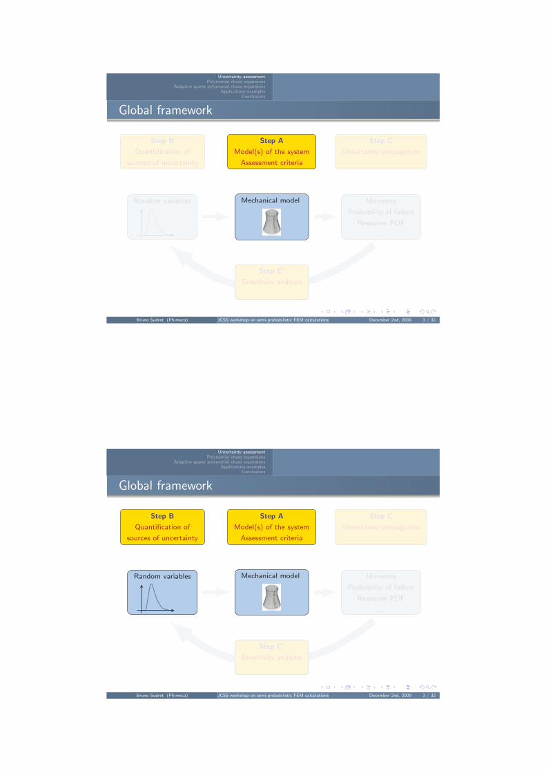
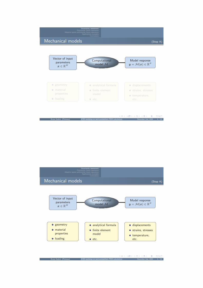
Global framework
Step A
Model(s) of the system
Assessment criteria
Step B
Quantification of
sources of uncertainty
Step C
Uncertainty propagation
Random variables Mechanical model Moments
Probability of failure
Response PDF
...
Step C’
Sensitivity analysis
Step C’
Sensitivity analysis
Bruno Sudret (Phimeca) JCSS workshop on semi-probabilistic FEM calculations December 2nd, 2009 3 / 32
Uncertainty assessmentPolynomial chaos expansions
Adaptive sparse polynomial chaos expansionsApplications examples
Conclusions
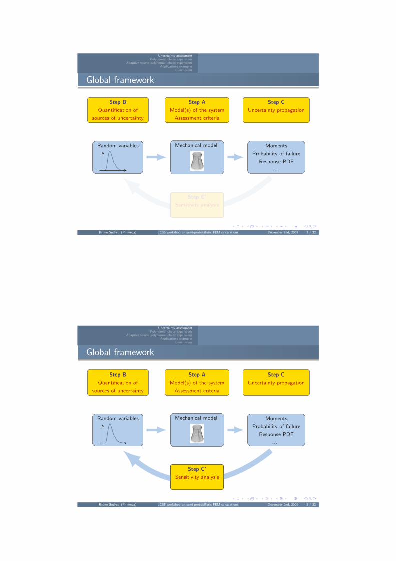
Mechanical models (Step A)
Computationalmodel M
Vector of inputparametersx ∈ R
M
Model responsey = M(x) ∈ R
N
geometry
materialproperties
loading
analytical formula
finite elementmodel
etc.
displacements
strains, stresses
temperature,etc.
Bruno Sudret (Phimeca) JCSS workshop on semi-probabilistic FEM calculations December 2nd, 2009 4 / 32
Uncertainty assessmentPolynomial chaos expansions
Adaptive sparse polynomial chaos expansionsApplications examples
Conclusions
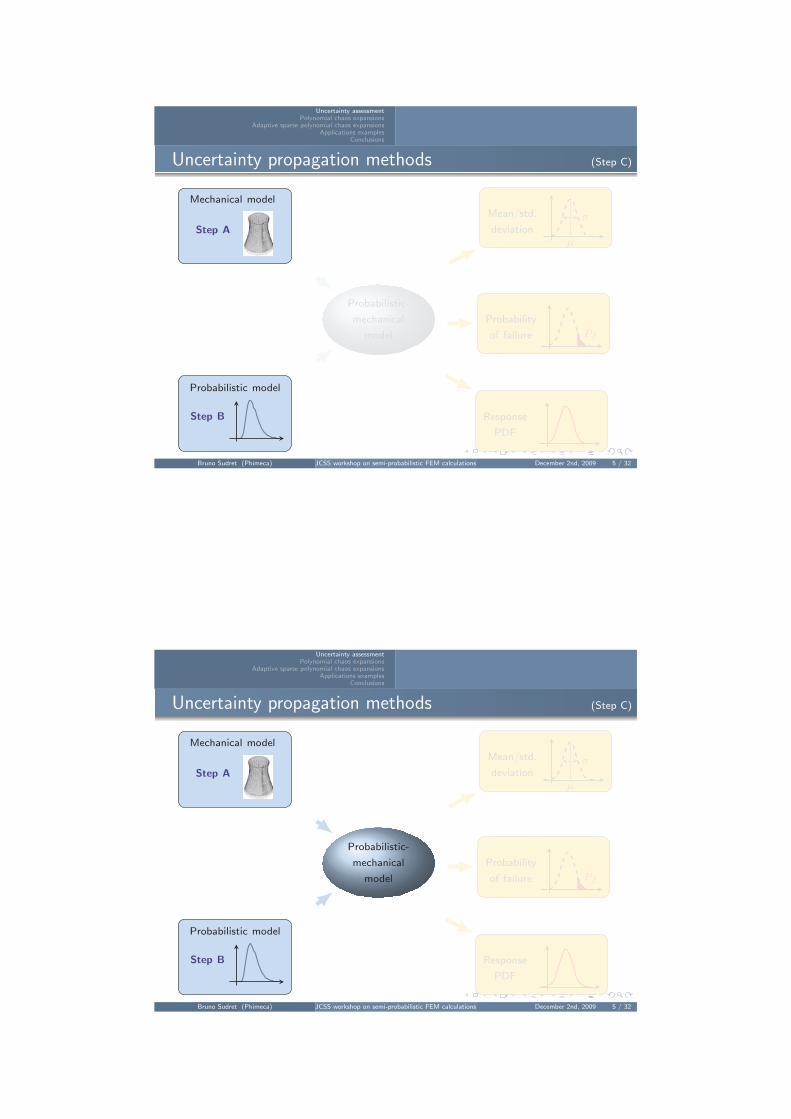
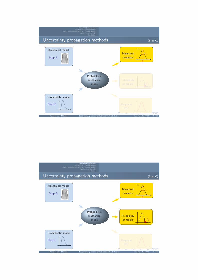
Uncertainty propagation methods (Step C)
Mechanical model
Step A
Mean/std.
deviationµ
σ
Probabilistic-
mechanical
model
Probability
of failure Pf
Probabilistic model
Step B Response
Bruno Sudret (Phimeca) JCSS workshop on semi-probabilistic FEM calculations December 2nd, 2009 5 / 32
Uncertainty assessmentPolynomial chaos expansions
Adaptive sparse polynomial chaos expansionsApplications examples
Conclusions
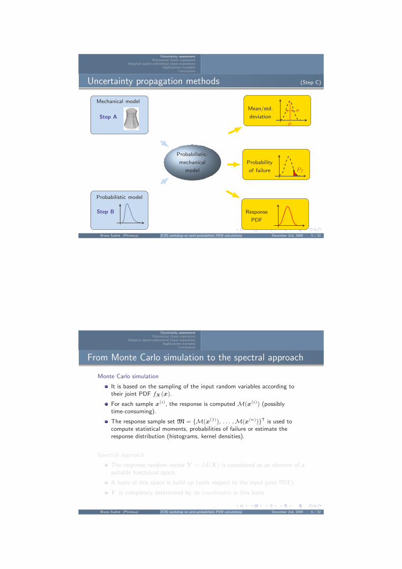
From Monte Carlo simulation to the spectral approach
Monte Carlo simulation
It is based on the sampling of the input random variables according totheir joint PDF fX (x).
For each sample x(i), the response is computed M(x(i)) (possiblytime-consuming).
The response sample set M = M(x(1)), . . . ,M(x(n))T is used tocompute statistical moments, probabilities of failure or estimate theresponse distribution (histograms, kernel densities).
Spectral approach
The response random vector Y = M(X) is considered as an element of asuitable functional space.
A basis of this space is build up (with respect to the input joint PDF).
Y is completely determined by its coordinates in this basis.
Bruno Sudret (Phimeca) JCSS workshop on semi-probabilistic FEM calculations December 2nd, 2009 6 / 32

Uncertainty assessmentPolynomial chaos expansions
Adaptive sparse polynomial chaos expansionsApplications examples
Conclusions
From Monte Carlo simulation to the spectral approach
Monte Carlo simulation
It is based on the sampling of the input random variables according totheir joint PDF fX (x).
For each sample x(i), the response is computed M(x(i)) (possiblytime-consuming).
The response sample set M = M(x(1)), . . . ,M(x(n))T is used tocompute statistical moments, probabilities of failure or estimate theresponse distribution (histograms, kernel densities).
Spectral approach
The response random vector Y = M(X) is considered as an element of asuitable functional space.
A basis of this space is build up (with respect to the input joint PDF).
Y is completely determined by its coordinates in this basis.
Bruno Sudret (Phimeca) JCSS workshop on semi-probabilistic FEM calculations December 2nd, 2009 6 / 32
Uncertainty assessmentPolynomial chaos expansions
Adaptive sparse polynomial chaos expansionsApplications examples
Conclusions
Generalized polynomial chaos basisComputation of the expansion coefficientsPost-processing of the coefficients
Principles
Random model response
Y = M(X) dim X = M, dim Y = 1
X : random vector of input parameters of prescribed PDF fX (X)
Y : scalar random response
If E[Y 2
]< ∞, then Y ∈ L2(Ω,F , PX ), the Hilbert space of second order
random variables equipped with the inner product < Y, Z >= E [Y Z]
Hilbertian basisY =
∑j∈IN
yj Ψj(X)
where:
Ψj(X): polynomial chaos basis
yj : “coordinates”, i.e. coefficients to be computed
Bruno Sudret (Phimeca) JCSS workshop on semi-probabilistic FEM calculations December 2nd, 2009 7 / 32
Uncertainty assessmentPolynomial chaos expansions
Adaptive sparse polynomial chaos expansionsApplications examples
Conclusions
Generalized polynomial chaos basisComputation of the expansion coefficientsPost-processing of the coefficients
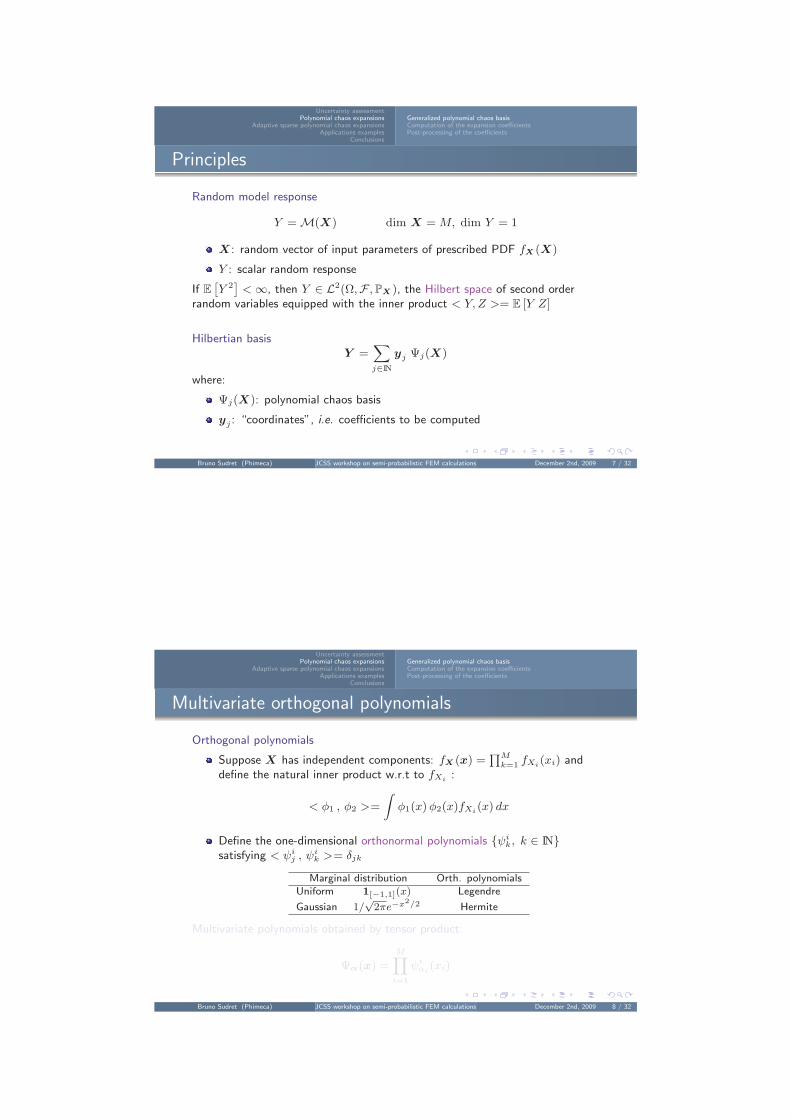
Multivariate orthogonal polynomials
Orthogonal polynomials
Suppose X has independent components: fX (x) =∏M
k=1 fXi(xi) anddefine the natural inner product w.r.t to fXi :
< φ1 , φ2 >=
∫φ1(x) φ2(x)fXi(x) dx
Define the one-dimensional orthonormal polynomials ψik, k ∈ IN
satisfying < ψij , ψi
k >= δjk
Marginal distribution Orth. polynomialsUniform 1[−1,1](x) Legendre
Gaussian 1/√
2πe−x2/2 Hermite
Multivariate polynomials obtained by tensor product:
Ψα(x) =
M∏i=1
ψiαi
(xi)
Bruno Sudret (Phimeca) JCSS workshop on semi-probabilistic FEM calculations December 2nd, 2009 8 / 32
Uncertainty assessmentPolynomial chaos expansions
Adaptive sparse polynomial chaos expansionsApplications examples
Conclusions
Generalized polynomial chaos basisComputation of the expansion coefficientsPost-processing of the coefficients
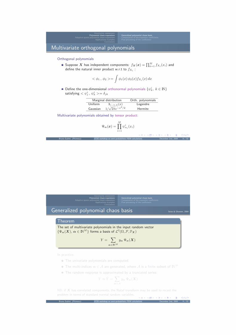
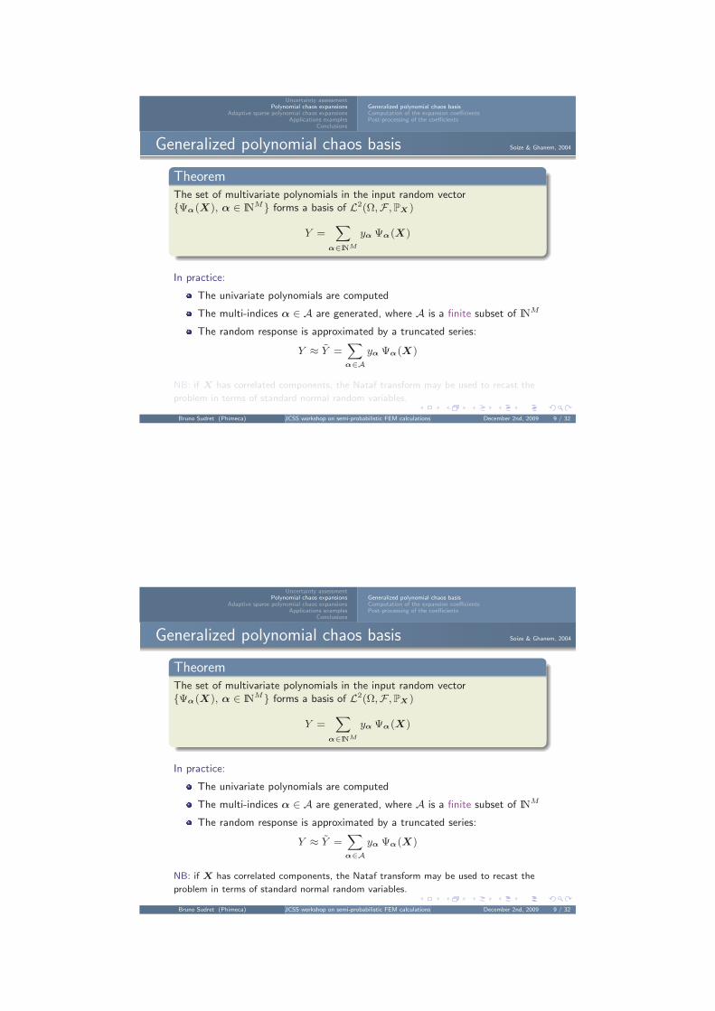
Generalized polynomial chaos basis Soize & Ghanem, 2004
TheoremThe set of multivariate polynomials in the input random vectorΨα(X), α ∈ INM forms a basis of L2(Ω,F , PX )
Y =∑
α∈INM
yα Ψα(X)
In practice:
The univariate polynomials are computed
The multi-indices α ∈ A are generated, where A is a finite subset of INM
The random response is approximated by a truncated series:
Y ≈ Y =∑α∈A
yα Ψα(X)
NB: if X has correlated components, the Nataf transform may be used to recast the
problem in terms of standard normal random variables.
Bruno Sudret (Phimeca) JCSS workshop on semi-probabilistic FEM calculations December 2nd, 2009 9 / 32
Uncertainty assessmentPolynomial chaos expansions
Adaptive sparse polynomial chaos expansionsApplications examples
Conclusions
Generalized polynomial chaos basisComputation of the expansion coefficientsPost-processing of the coefficients
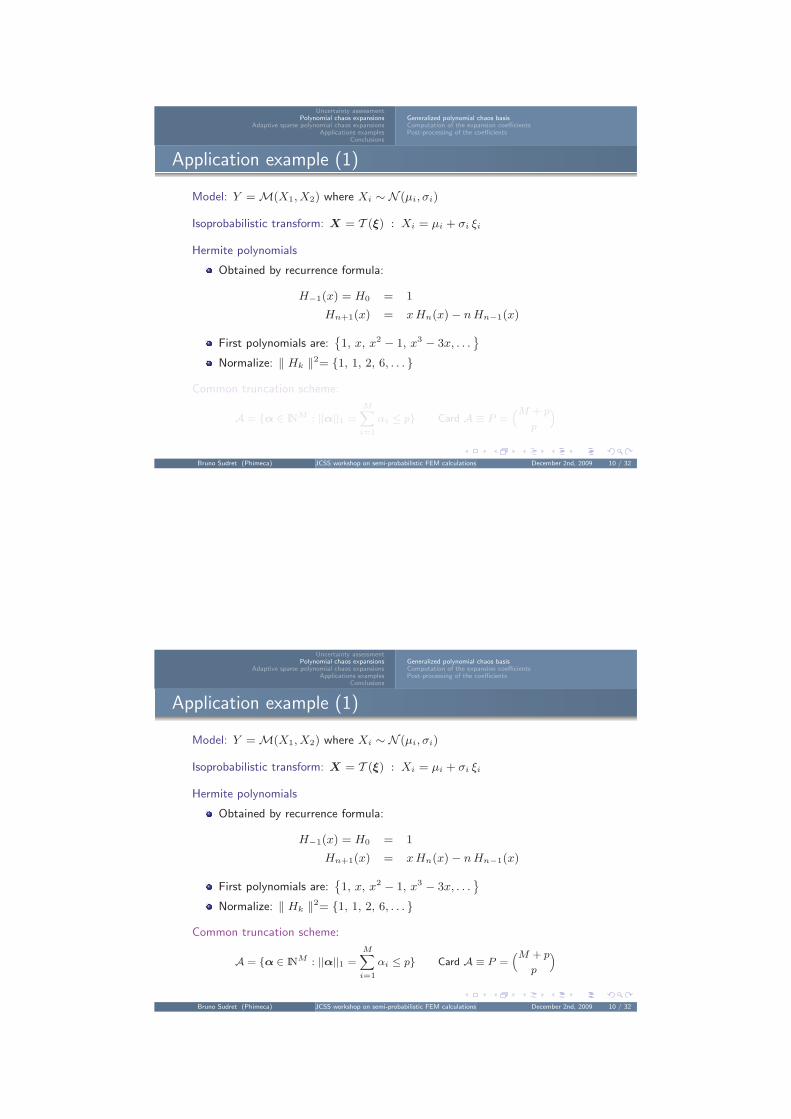
Application example (1)
Model: Y = M(X1, X2) where Xi ∼ N (µi, σi)
Isoprobabilistic transform: X = T (ξ) : Xi = µi + σi ξi
Hermite polynomials
Obtained by recurrence formula:
H−1(x) = H0 = 1
Hn+1(x) = x Hn(x) − n Hn−1(x)
First polynomials are:1, x, x2 − 1, x3 − 3x, . . .
Normalize: ‖ Hk ‖2= 1, 1, 2, 6, . . .
Common truncation scheme:
A = α ∈ INM : ||α||1 =
M∑i=1
αi ≤ p Card A ≡ P =(M + p
p
)
Bruno Sudret (Phimeca) JCSS workshop on semi-probabilistic FEM calculations December 2nd, 2009 10 / 32
Uncertainty assessmentPolynomial chaos expansions
Adaptive sparse polynomial chaos expansionsApplications examples
Conclusions
Generalized polynomial chaos basisComputation of the expansion coefficientsPost-processing of the coefficients
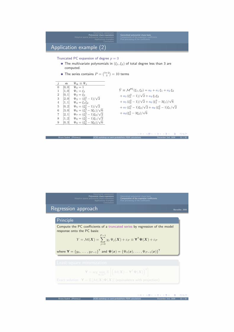
Application example (2)
Truncated PC expansion of degree p = 3
The multivariate polynomials in (ξ1, ξ2) of total degree less than 3 arecomputed.
The series contains P =(3+23
)= 10 terms
j α Ψα ≡ Ψj
0 [0, 0] Ψ0 = 11 [1, 0] Ψ1 = ξ12 [0, 1] Ψ2 = ξ23 [2, 0] Ψ3 = (ξ2
1 − 1)/√
24 [1, 1] Ψ4 = ξ1ξ25 [0, 2] Ψ5 = (ξ2
2 − 1)/√
2
6 [3, 0] Ψ6 = (ξ31 − 3ξ1)/
√6
7 [2, 1] Ψ7 = (ξ21 − 1)ξ2/
√2
8 [1, 2] Ψ8 = (ξ22 − 1)ξ1/
√2
9 [0, 3] Ψ9 = (ξ32 − 3ξ2)/
√6
Y ≡ MPC(ξ1, ξ2) = a0 + a1 ξ1 + a2 ξ2
+ a3 (ξ21 − 1)/
√2 + a4 ξ1ξ2
+ a5 (ξ22 − 1)/
√2 + a6 (ξ3
1 − 3ξ1)/√
6
+ a7 (ξ21 − 1)ξ2/
√2 + a8 (ξ2
2 − 1)ξ1/√
2
+ a9(ξ32 − 3ξ2)/
√6
Bruno Sudret (Phimeca) JCSS workshop on semi-probabilistic FEM calculations December 2nd, 2009 11 / 32
Uncertainty assessmentPolynomial chaos expansions
Adaptive sparse polynomial chaos expansionsApplications examples
Conclusions
Generalized polynomial chaos basisComputation of the expansion coefficientsPost-processing of the coefficients
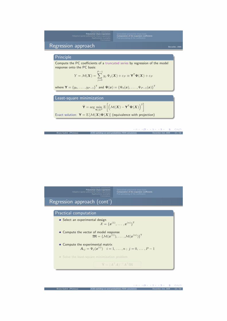
Regression approach Berveiller, 2005
PrincipleCompute the PC coefficients of a truncated series by regression of the modelresponse onto the PC basis:
Y = M(X) =
P−1∑j=0
yj Ψj(X) + εP ≡ YTΨ(X) + εP
where Y = y0, . . . , yP−1T and Ψ(x) = Ψ0(x), . . . , ΨP−1(x)T
Least-square minimization
Y = arg minY∈RP
E
[(M(X) − YTΨ(X)
)2]
Exact solution: Y = E [M(X)Ψ(X)] (equivalence with projection)
Bruno Sudret (Phimeca) JCSS workshop on semi-probabilistic FEM calculations December 2nd, 2009 12 / 32
Uncertainty assessmentPolynomial chaos expansions
Adaptive sparse polynomial chaos expansionsApplications examples
Conclusions
Generalized polynomial chaos basisComputation of the expansion coefficientsPost-processing of the coefficients
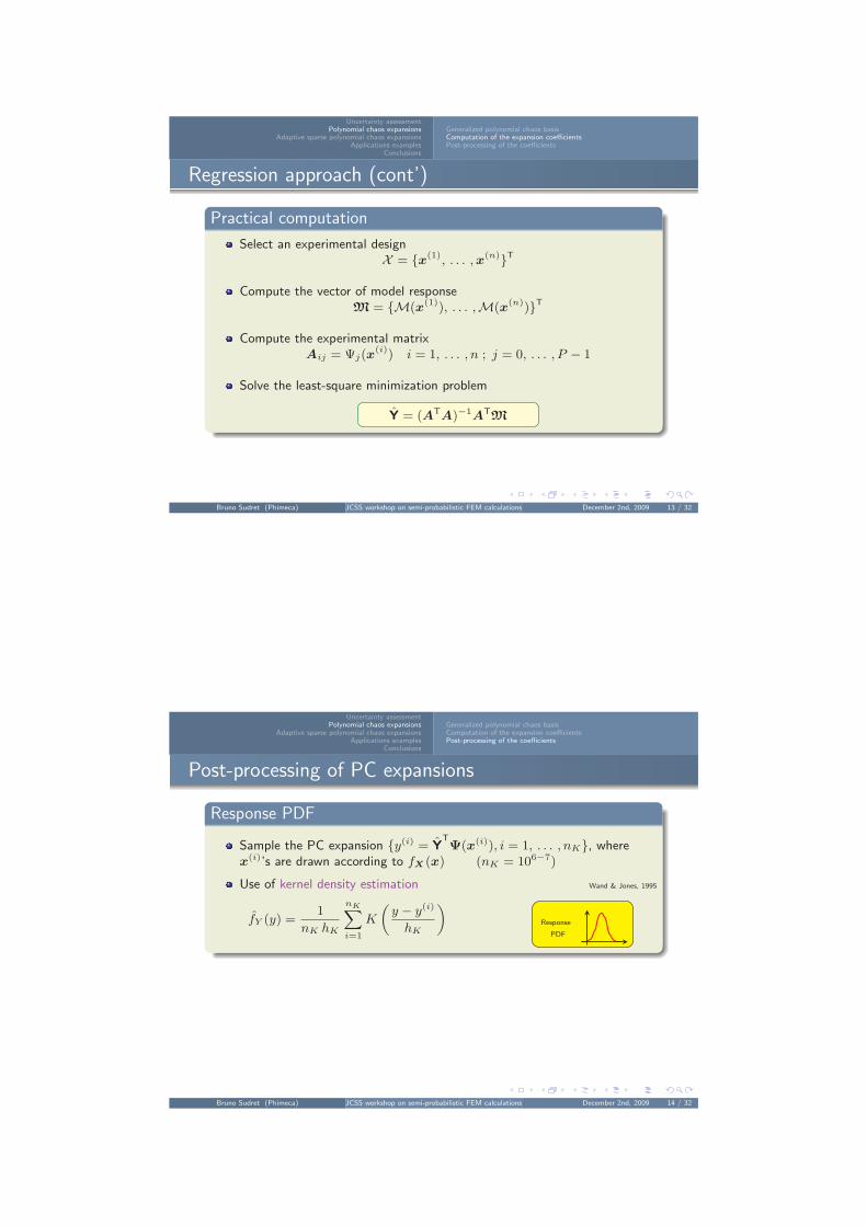
Regression approach (cont’)
Practical computation
Select an experimental designX = x(1), . . . , x(n)T
Compute the vector of model responseM = M(x(1)), . . . ,M(x(n))T
Compute the experimental matrixAij = Ψj(x
(i)) i = 1, . . . , n ; j = 0, . . . , P − 1
Solve the least-square minimization problem
Y = (ATA)−1ATM
Bruno Sudret (Phimeca) JCSS workshop on semi-probabilistic FEM calculations December 2nd, 2009 13 / 32
Uncertainty assessmentPolynomial chaos expansions
Adaptive sparse polynomial chaos expansionsApplications examples
Conclusions
Generalized polynomial chaos basisComputation of the expansion coefficientsPost-processing of the coefficients
Post-processing of PC expansions
Response PDF
Sample the PC expansion y(i) = YTΨ(x(i)), i = 1, . . . , nK, where
x(i)’s are drawn according to fX (x) (nK = 106−7)
Use of kernel density estimation Wand & Jones, 1995
fY (y) =1
nK hK
nK∑i=1
K
(y − y(i)
hK
)Response
Bruno Sudret (Phimeca) JCSS workshop on semi-probabilistic FEM calculations December 2nd, 2009 14 / 32
Uncertainty assessmentPolynomial chaos expansions
Adaptive sparse polynomial chaos expansionsApplications examples
Conclusions
Generalized polynomial chaos basisComputation of the expansion coefficientsPost-processing of the coefficients
Post-processing of PC expansions
Response PDF
Sample the PC expansion y(i) = YTΨ(x(i)), i = 1, . . . , nK, where
x(i)’s are drawn according to fX (x) (nK = 106−7)
Use of kernel density estimation Wand & Jones, 1995
fY (y) =1
nK hK
nK∑i=1
K
(y − y(i)
hK
)Response
Statistical momentsµPC
Y ≡ E [Y ] = y0
σ2,PCY ≡ Var [Y ] =
P−1∑j=1
y2j
...
Mean/std.
deviationµ
σ
Bruno Sudret (Phimeca) JCSS workshop on semi-probabilistic FEM calculations December 2nd, 2009 14 / 32
Uncertainty assessmentPolynomial chaos expansions
Adaptive sparse polynomial chaos expansionsApplications examples
Conclusions
Generalized polynomial chaos basisComputation of the expansion coefficientsPost-processing of the coefficients
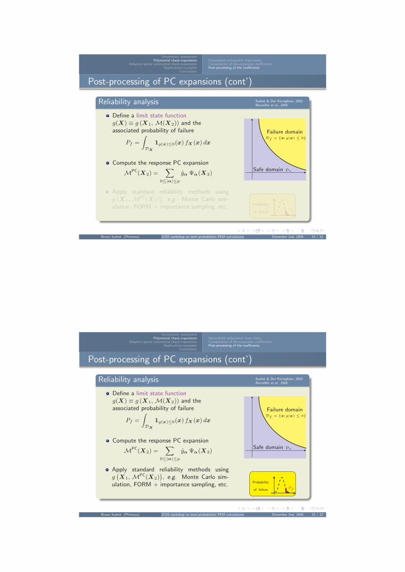
Post-processing of PC expansions (cont’)
Reliability analysis Sudret & Der Kiureghian, 2002Berveiller et al., 2005
Define a limit state functiong(X) ≡ g (X1, M(X2)) and theassociated probability of failure
Pf =
∫DX
1g(x)≤0(x) fX (x) dx
Compute the response PC expansion
MPC(X2) =∑
0≤|α|≤p
yα Ψα(X2)
Failure domainDf = x:g(x) ≤ 0
Safe domain Ds
Apply standard reliability methods usingg
(X1, MPC(X2)
), e.g. Monte Carlo sim-
ulation, FORM + importance sampling, etc. Probability
of failurePf
Bruno Sudret (Phimeca) JCSS workshop on semi-probabilistic FEM calculations December 2nd, 2009 15 / 32
Uncertainty assessmentPolynomial chaos expansions
Adaptive sparse polynomial chaos expansionsApplications examples
Conclusions
Generalized polynomial chaos basisComputation of the expansion coefficientsPost-processing of the coefficients
Post-processing of PC expansions (cont’)
Reliability analysis Sudret & Der Kiureghian, 2002Berveiller et al., 2005
Define a limit state functiong(X) ≡ g (X1, M(X2)) and theassociated probability of failure
Pf =
∫DX
1g(x)≤0(x) fX (x) dx
Compute the response PC expansion
MPC(X2) =∑
0≤|α|≤p
yα Ψα(X2)
Failure domainDf = x:g(x) ≤ 0
Safe domain Ds
Apply standard reliability methods usingg
(X1, MPC(X2)
), e.g. Monte Carlo sim-
ulation, FORM + importance sampling, etc. Probability
of failurePf
Bruno Sudret (Phimeca) JCSS workshop on semi-probabilistic FEM calculations December 2nd, 2009 15 / 32
Uncertainty assessmentPolynomial chaos expansions
Adaptive sparse polynomial chaos expansionsApplications examples
Conclusions
Error estimators and sparse truncation schemesAdaptive algorithms
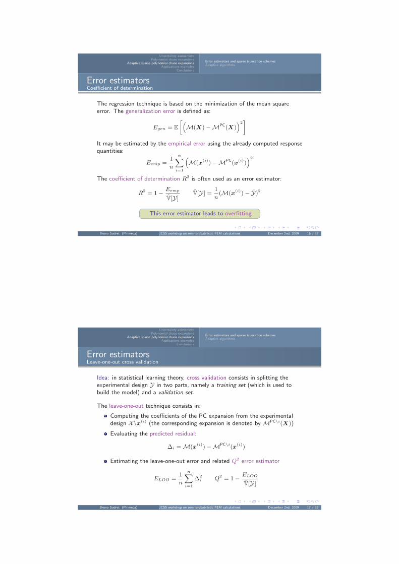
Error estimatorsCoefficient of determination
The regression technique is based on the minimization of the mean squareerror. The generalization error is defined as:
Egen = E
[(M(X) −MPC(X)
)2]
It may be estimated by the empirical error using the already computed responsequantities:
Eemp =1
n
n∑i=1
(M(x(i)) −MPC(x(i))
)2
The coefficient of determination R2 is often used as an error estimator:
R2 = 1 − Eemp
V[Y]V[Y] =
1
n(M(x(i)) − Y)2
This error estimator leads to overfitting
Bruno Sudret (Phimeca) JCSS workshop on semi-probabilistic FEM calculations December 2nd, 2009 16 / 32
Uncertainty assessmentPolynomial chaos expansions
Adaptive sparse polynomial chaos expansionsApplications examples
Conclusions
Error estimators and sparse truncation schemesAdaptive algorithms
Error estimatorsLeave-one-out cross validation
Idea: in statistical learning theory, cross validation consists in splitting theexperimental design Y in two parts, namely a training set (which is used tobuild the model) and a validation set.
The leave-one-out technique consists in:
Computing the coefficients of the PC expansion from the experimentaldesign X\x(i) (the corresponding expansion is denoted by MPC\i(X))
Evaluating the predicted residual:
∆i = M(x(i)) −MPC\i(x(i))
Estimating the leave-one-out error and related Q2 error estimator
ELOO =1
n
n∑i=1
∆2i Q2 = 1 − ELOO
V[Y]
Bruno Sudret (Phimeca) JCSS workshop on semi-probabilistic FEM calculations December 2nd, 2009 17 / 32
Uncertainty assessmentPolynomial chaos expansions
Adaptive sparse polynomial chaos expansionsApplications examples
Conclusions
Error estimators and sparse truncation schemesAdaptive algorithms
The curse of dimensionality
Common truncation scheme: all the multivariate polynomials up to aprescribed order p are selected. The number of unknown coefficients growthspolynomially both in M and p.
P =
(M + p
p
)
So does the size of experimental design, e.g. n = 2P when using Latinhypercube sampling.
“Full” expansions are not tractable when M ≥ 10
Solutions:
sparse truncation schemes, based on the sparsity-of-effect principle
adaptive algorithms for the construction of the PC expansion
Bruno Sudret (Phimeca) JCSS workshop on semi-probabilistic FEM calculations December 2nd, 2009 18 / 32
Uncertainty assessmentPolynomial chaos expansions
Adaptive sparse polynomial chaos expansionsApplications examples
Conclusions
Error estimators and sparse truncation schemesAdaptive algorithms
Hyperbolic truncation schemes
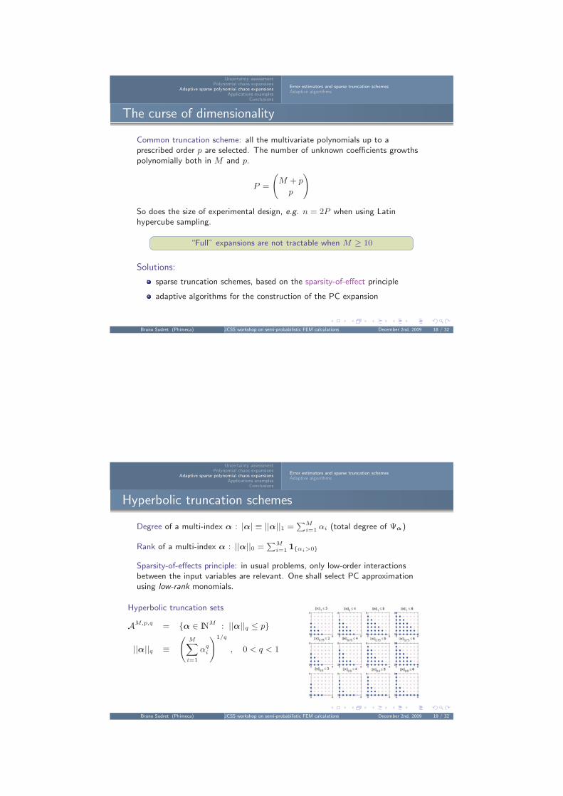
Degree of a multi-index α : |α| ≡ ||α||1 =∑M
i=1 αi (total degree of Ψα)
Rank of a multi-index α : ||α||0 =∑M
i=1 1αi>0
Sparsity-of-effects principle: in usual problems, only low-order interactionsbetween the input variables are relevant. One shall select PC approximationusing low-rank monomials.
Hyperbolic truncation sets
AM,p,q = α ∈ INM : ||α||q ≤ p
||α||q ≡(
M∑i=1
αqi
)1/q
, 0 < q < 1
Bruno Sudret (Phimeca) JCSS workshop on semi-probabilistic FEM calculations December 2nd, 2009 19 / 32
Uncertainty assessmentPolynomial chaos expansions
Adaptive sparse polynomial chaos expansionsApplications examples
Conclusions
Error estimators and sparse truncation schemesAdaptive algorithms
Adaptive algorithm: principles
Adaptivity in the PC basis:
Build up the polynomial chaos basis from scratch, i.e. starting with asingle constant term, using an iterative algorithm
Add monomial terms (that are selected using the hyperbolic truncationscheme) one-by-one and decide whether they are kept or discarded (R2
coefficient is used)
Monitor the PC error using cross-validation (Q2 estimate) and stop whenQ2
tgt is attained.
Adaptivity in the experimental design:
In each step, the PC coefficients are computed by regression. Nestedexperimental designs (e.g. quasi-random numbers, nested LHS) are usedin order to make the regression problem well-posed.
Bruno Sudret (Phimeca) JCSS workshop on semi-probabilistic FEM calculations December 2nd, 2009 20 / 32
Uncertainty assessmentPolynomial chaos expansions
Adaptive sparse polynomial chaos expansionsApplications examples
Conclusions
Error estimators and sparse truncation schemesAdaptive algorithms
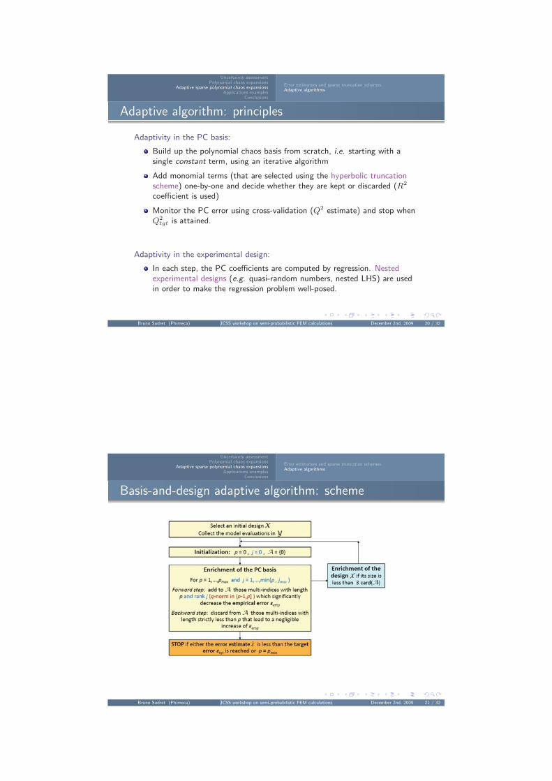
Basis-and-design adaptive algorithm: scheme
Bruno Sudret (Phimeca) JCSS workshop on semi-probabilistic FEM calculations December 2nd, 2009 21 / 32
Uncertainty assessmentPolynomial chaos expansions
Adaptive sparse polynomial chaos expansionsApplications examples
Conclusions
Elastic trussFrame structureFoundation with spatial variability
Elastic truss Blatman et al., 2007
Problem statement
10 independent random variables
4 section/material properties(lognormal)
6 loads (Gumbel)
Use of Hermite polynomial chaos
Response quantity: vertical displacement at midspan
Reliability problem:
g(X) = vmax − v(X) = vmax − FEM(E1, A1, E2, A2, P1, . . . , P6)
Bruno Sudret (Phimeca) JCSS workshop on semi-probabilistic FEM calculations December 2nd, 2009 22 / 32
Uncertainty assessmentPolynomial chaos expansions
Adaptive sparse polynomial chaos expansionsApplications examples
Conclusions
Elastic trussFrame structureFoundation with spatial variability
Structural reliability results (adaptive algorithm)
Threshold (cm) Reference Full PCE Sparse PCE
βREF β ε (%) β ε (%)
10 1.72 1.71 0.6 1.72 0.011 2.38 2.38 0.0 2.38 0.012 2.97 2.98 0.3 2.99 0.714 3.98 4.04 1.5 4.07 2.316 4.85 4.95 2.1 5.02 3.5
1 − Q2 1 · 10−6 9 · 10−5
Number of terms 286 114Number of FE runs 443 207
Using ∼ 200 finite element runs, the structural reliability problem with various
thresholds is solved accurately up to β = 5.
Bruno Sudret (Phimeca) JCSS workshop on semi-probabilistic FEM calculations December 2nd, 2009 23 / 32
Uncertainty assessmentPolynomial chaos expansions
Adaptive sparse polynomial chaos expansionsApplications examples
Conclusions
Elastic trussFrame structureFoundation with spatial variability
PDF of the maximal deflection
Using ∼ 200 finite element runs, the PDF of the maximal deflection is
accurately computed in the central part as well as in the tails.
Bruno Sudret (Phimeca) JCSS workshop on semi-probabilistic FEM calculations December 2nd, 2009 24 / 32
Uncertainty assessmentPolynomial chaos expansions
Adaptive sparse polynomial chaos expansionsApplications examples
Conclusions
Elastic trussFrame structureFoundation with spatial variability
Frame under lateral loads
Problem statement
21 correlated randomvariables:
2 Young’s moduli(truncated Gaussian)
8 cross sections and 8moments of inertia(truncated Gaussian)
3 loads (lognormal)
Use of Nataf transform and Hermite polynomial chaos
Bruno Sudret (Phimeca) JCSS workshop on semi-probabilistic FEM calculations December 2nd, 2009 25 / 32
Uncertainty assessmentPolynomial chaos expansions
Adaptive sparse polynomial chaos expansionsApplications examples
Conclusions
Elastic trussFrame structureFoundation with spatial variability
Structural reliability results (adaptive algorithm)
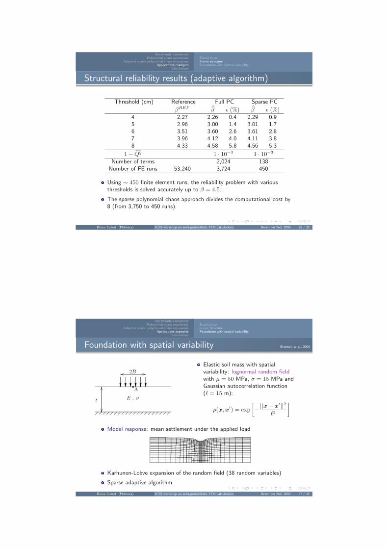
Threshold (cm) Reference Full PC Sparse PC
βREF β ε (%) β ε (%)
4 2.27 2.26 0.4 2.29 0.95 2.96 3.00 1.4 3.01 1.76 3.51 3.60 2.6 3.61 2.87 3.96 4.12 4.0 4.11 3.88 4.33 4.58 5.8 4.56 5.3
1 − Q2 1 · 10−3 1 · 10−3
Number of terms 2,024 138Number of FE runs 53,240 3,724 450
Using ∼ 450 finite element runs, the reliability problem with variousthresholds is solved accurately up to β = 4.5.
The sparse polynomial chaos approach divides the computational cost by8 (from 3,750 to 450 runs).
Bruno Sudret (Phimeca) JCSS workshop on semi-probabilistic FEM calculations December 2nd, 2009 26 / 32
Uncertainty assessmentPolynomial chaos expansions
Adaptive sparse polynomial chaos expansionsApplications examples
Conclusions
Elastic trussFrame structureFoundation with spatial variability
Foundation with spatial variability Blatman et al., 2009
Elastic soil mass with spatialvariability: lognormal random fieldwith µ = 50 MPa, σ = 15 MPa andGaussian autocorrelation function( = 15 m):
ρ(x, x′) = exp
[−||x − x′||2
2
]
Model response: mean settlement under the applied load
Karhunen-Loeve expansion of the random field (38 random variables)
Sparse adaptive algorithm
Bruno Sudret (Phimeca) JCSS workshop on semi-probabilistic FEM calculations December 2nd, 2009 27 / 32
Uncertainty assessmentPolynomial chaos expansions
Adaptive sparse polynomial chaos expansionsApplications examples
Conclusions
Elastic trussFrame structureFoundation with spatial variability
Foundation - Results (1)
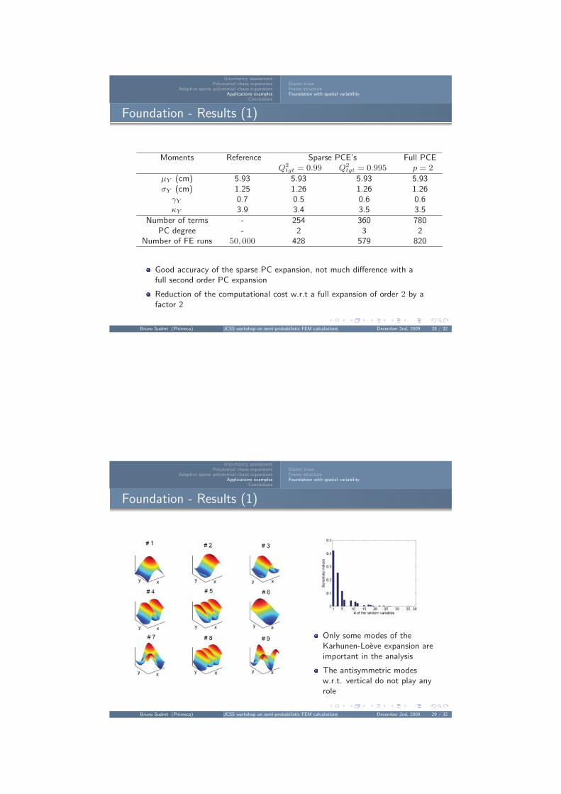
Moments Reference Sparse PCE’s Full PCEQ2
tgt = 0.99 Q2tgt = 0.995 p = 2
µY (cm) 5.93 5.93 5.93 5.93σY (cm) 1.25 1.26 1.26 1.26
γY 0.7 0.5 0.6 0.6κY 3.9 3.4 3.5 3.5
Number of terms - 254 360 780PC degree - 2 3 2
Number of FE runs 50, 000 428 579 820
Good accuracy of the sparse PC expansion, not much difference with afull second order PC expansion
Reduction of the computational cost w.r.t a full expansion of order 2 by afactor 2
Bruno Sudret (Phimeca) JCSS workshop on semi-probabilistic FEM calculations December 2nd, 2009 28 / 32
Uncertainty assessmentPolynomial chaos expansions
Adaptive sparse polynomial chaos expansionsApplications examples
Conclusions
Elastic trussFrame structureFoundation with spatial variability
Foundation - Results (1)
Only some modes of theKarhunen-Loeve expansion areimportant in the analysis
The antisymmetric modesw.r.t. vertical do not play anyrole
Bruno Sudret (Phimeca) JCSS workshop on semi-probabilistic FEM calculations December 2nd, 2009 29 / 32
Uncertainty assessmentPolynomial chaos expansions
Adaptive sparse polynomial chaos expansionsApplications examples
Conclusions
Elastic trussFrame structureFoundation with spatial variability
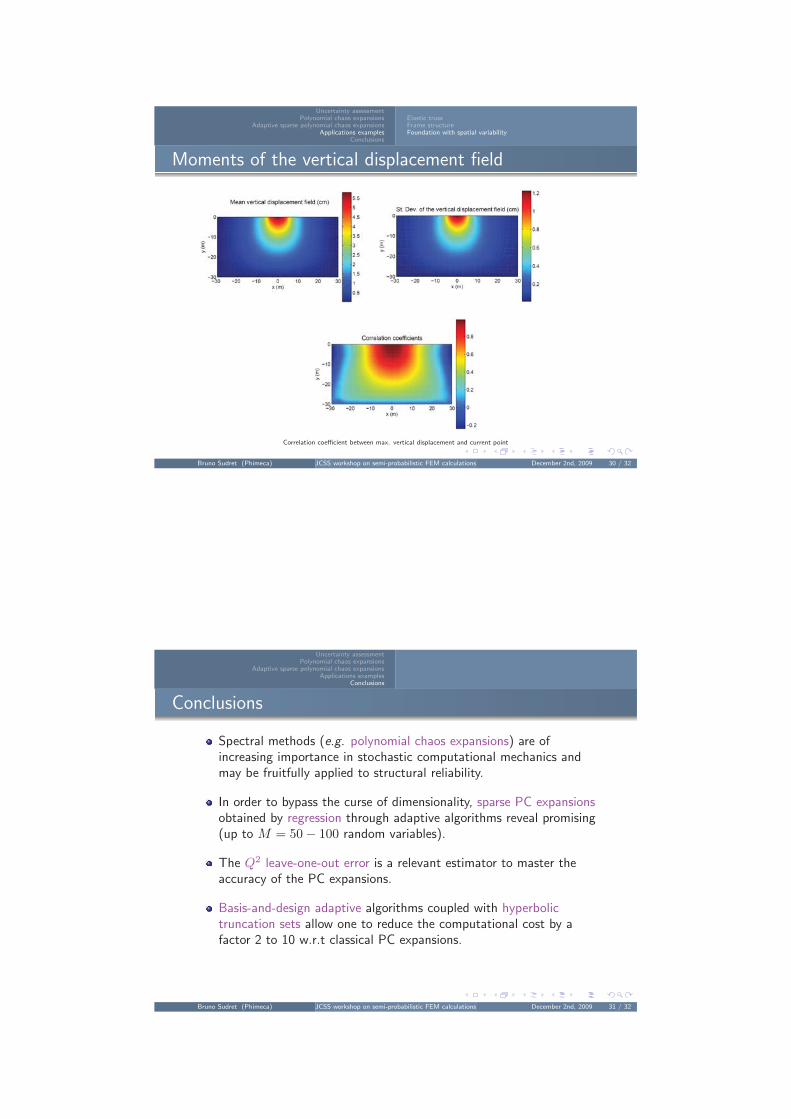
Moments of the vertical displacement field
Correlation coefficient between max. vertical displacement and current point
Bruno Sudret (Phimeca) JCSS workshop on semi-probabilistic FEM calculations December 2nd, 2009 30 / 32
Uncertainty assessmentPolynomial chaos expansions
Adaptive sparse polynomial chaos expansionsApplications examples
Conclusions
Conclusions
Spectral methods (e.g. polynomial chaos expansions) are ofincreasing importance in stochastic computational mechanics andmay be fruitfully applied to structural reliability.
In order to bypass the curse of dimensionality, sparse PC expansionsobtained by regression through adaptive algorithms reveal promising(up to M = 50 − 100 random variables).
The Q2 leave-one-out error is a relevant estimator to master theaccuracy of the PC expansions.
Basis-and-design adaptive algorithms coupled with hyperbolictruncation sets allow one to reduce the computational cost by afactor 2 to 10 w.r.t classical PC expansions.
Bruno Sudret (Phimeca) JCSS workshop on semi-probabilistic FEM calculations December 2nd, 2009 31 / 32

Uncertainty assessmentPolynomial chaos expansions
Adaptive sparse polynomial chaos expansionsApplications examples
Conclusions
Thank you very much for your attention!
Acknowlegment: The partnership between Phimeca, IFMA/LaMI and EDF R&D
under Contract # 8610-AAP-5910049992 is gratefully acknowledged.
Bruno Sudret (Phimeca) JCSS workshop on semi-probabilistic FEM calculations December 2nd, 2009 32 / 32
Uncertainty assessmentPolynomial chaos expansions
Adaptive sparse polynomial chaos expansionsApplications examples
Conclusions
References
Berveiller, M. (2005).
Elements finis stochastiques : approches intrusive et non intrusive pour des analyses de fiabilite.Ph. D. thesis, Universite Blaise Pascal, Clermont-Ferrand.
Blatman, G. (2009).
Adaptive sparse polynomial chaos expansions for uncertainty propagation and sensitivity analysis.Ph. D. thesis, Universite Blaise Pascal, Clermont-Ferrand.in preparation.
Blatman, G. and B. Sudret (2008).
Sparse polynomial chaos expansions and adaptive stochastic finite elements using a regression approach.Comptes Rendus Mecanique 336(6), 518–523.
Blatman, G. and B. Sudret (2009).
Use of sparse polynomial chaos expansions in adaptive stochastic finite element analysis.Prob. Eng. Mech..(In press).
Soize, C. and R. Ghanem (2004).
Physical systems with random uncertainties: chaos representations with arbitrary probability measure.SIAM J. Sci. Comput. 26(2), 395–410.
Sudret, B. (2007).
Uncertainty propagation and sensitivity analysis in mechanical models – Contributions to structural reliability and stochasticspectral methods.Habilitation a diriger des recherches, Universite Blaise Pascal, Clermont-Ferrand, France.
Bruno Sudret (Phimeca) JCSS workshop on semi-probabilistic FEM calculations December 2nd, 2009 32 / 32
Recommended