Embed Size (px)
Citation preview

U.S. Department of the InteriorU.S. Geological Survey
Circular 1413
Developing Integrated Methods to Address Complex Resource and Environmental Issues
Geophysics
Remote Sensing
Geochemistry

Front cover. Top photograph, Jonathan Caine drilling a stilling well for a streamgage in upper Handcart Gulch, Colo. (USGS photograph) Middle photograph, Ships and relief drill rigs working to intersect and seal the Macondo well during the Deepwater Horizon oil spill, July 9, 2010. (Photograph by Gregg Swayze, USGS) Bottom photograph, Benjamin Drenth measuring strength of the Earth’s gravity field at Great Dunes National Park, June 2011. (Photograph by David V. Fitterman)Back cover. Seth Haines doing field work near Isabella Dam, above Bakersfield, Calif., February 2007. (Photograph by Bethany Burton)

Developing Integrated Methods to Address Complex Resource and Environmental Issues
Edited by Kathleen S. Smith, Jeffrey D. Phillips, Anne E. McCafferty, and Roger N. Clark
Circular 1413
U.S. Department of the InteriorU.S. Geological Survey

U.S. Department of the InteriorSALLY JEWELL, Secretary
U.S. Geological SurveySuzette M. Kimball, Director
U.S. Geological Survey, Reston, Virginia: 2016
For more information on the USGS—the Federal source for science about the Earth, its natural and living resources, natural hazards, and the environment—visit http://www.usgs.gov or call 1–888–ASK–USGS.
For an overview of USGS information products, including maps, imagery, and publications, visit http://www.usgs.gov/pubprod/.
Any use of trade, firm, or product names is for descriptive purposes only and does not imply endorsement by the U.S. Government.
Although this information product, for the most part, is in the public domain, it also may contain copyrighted materials as noted in the text. Permission to reproduce copyrighted items must be secured from the copyright owner.
Suggested citation:Smith, K.S., Phillips, J.D., McCafferty, A.E., and Clark, R.N., eds., 2016, Developing integrated methods to address complex resource and environmental issues: U.S. Geological Survey Circular 1413, 160 p., http://dx.doi.org/10.3133/cir1413.
Library of Congress Cataloging-in-Publication Data
Developing integrated methods to address complex resource and environmental issues / edited by Kathleen S. Smith, Jeffrey D. Phillips, Anne E. McCafferty, and Roger N. Clark. pages cm. -- (Circular ; 1413) Includes bibliographical references. ISBN 978-1-4113-3969-9 (pbk.) 1. Geophysics. 2. Geodynamics. 3. Earth sciences. 4. Environmental risk assessment. I. Smith, Kathleen S. (Geologist) II. Phillips, Jeffrey D. III. McCafferty, Anne. IV. Clark, Roger N. (Roger Nelson) QE501.D485 2015 550--dc23 2015035017
ISSN 1067-084X (print) ISSN 2330-5703 (online)ISBN 978-1-4113-3969-9

iii
Conversion FactorsSI to Inch/Pound
Multiply By To obtainLength
centimeter (cm) 0.3937 inch (in.)millimeter (mm) 0.03937 inch (in.)meter (m) 3.281 foot (ft) kilometer (km) 0.6214 mile (mi)meter (m) 1.094 yard (yd)
Areasquare meter (m2) 0.0002471 acre square kilometer (km2) 247.1 acresquare centimeter (cm2) 0.001076 square foot (ft2)square meter (m2) 10.76 square foot (ft2) square centimeter (cm2) 0.1550 square inch (ft2) square kilometer (km2) 0.3861 square mile (mi2)
Volumeliter (L) 33.82 ounce, fluid (fl. oz)liter (L) 0.2642 gallon (gal)cubic meter (m3) 264.2 gallon (gal) cubic decimeter (dm3) 0.2642 gallon (gal) cubic meter (m3) 0.0002642 million gallons (Mgal) cubic centimeter (cm3) 0.06102 cubic inch (in3) cubic decimeter (dm3) 61.02 cubic inch (in3) liter (L) 61.02 cubic inch (in3) cubic decimeter (dm3) 0.03531 cubic foot (ft3) cubic meter (m3) 35.31 cubic foot (ft3)cubic meter (m3) 1.308 cubic yard (yd3) cubic kilometer (km3) 0.2399 cubic mile (mi3)
Flow ratemeter per second (m/s) 3.281 foot per second (ft/s) meter per minute (m/min) 3.281 foot per minute (ft/min) meter per hour (m/hr) 3.281 foot per hour (ft/hr)meter per day (m/d) 3.281 foot per day (ft/d)meter per year (m/yr) 3.281 foot per year ft/yr) cubic meter per second (m3/s) 35.31 cubic foot per second (ft3/s)cubic meter per second per
square kilometer [(m3/s)/km2]91.49 cubic foot per second per square mile [(ft3/s)/mi2]
cubic meter per day (m3/d) 35.31 cubic foot per day (ft3/d) liter per second (L/s) 15.85 gallon per minute (gal/min) cubic meter per day (m3/d) 264.2 gallon per day (gal/d) cubic meter per second (m3/s) 22.83 million gallons per day (Mgal/d) kilometer per hour (km/h) 0.6214 mile per hour (mi/h)
Massgram (g) 0.03527 ounce, avoirdupois (oz)kilogram (kg) 2.205 pound avoirdupois (lb)megagram (Mg) 1.102 ton, short (2,000 lb)megagram (Mg) 0.9842 ton, long (2,240 lb)metric ton per day 1.102 ton per day (ton/d)

iv
Magnetic susceptibilitymagnetic susceptibility (SI) 1/(4π)=0.079577 magnetic susceptibility (cgs or electromagnetic
unit per cubic centimeter [emu/cm3])Density
kilogram per cubic meter (kg/m3) 0.001 grams per cubic centimeter (g/cm3) Hydraulic conductivity
meter per day (m/d) 3.281 foot per day (ft/d) Hydraulic gradient
meter per kilometer (m/km) 5.27983 foot per mile (ft/mi) Transmissivity*
meter squared per day (m2/d) 10.76 foot squared per day (ft2/d)
Temperature in degrees Celsius (°C) may be converted to degrees Fahrenheit (°F) as follows:
°F=(1.8×°C)+32
Temperature in degrees Fahrenheit (°F) may be converted to degrees Celsius (°C) as follows:
°C=(°F-32)/1.8
Vertical coordinate information is referenced to the insert datum name (and abbreviation) here, for instance, “North American Vertical Datum of 1988 (NAVD 88)”
Horizontal coordinate information is referenced to the insert datum name (and abbreviation) here, for instance, “North American Datum of 1983 (NAD 83)”
Altitude, as used in this report, refers to distance above the vertical datum.
*Transmissivity: The standard unit for transmissivity is cubic foot per day per square foot times foot of aquifer thickness [(ft3/d)/ft2]ft. In this report, the mathematically reduced form, foot squared per day (ft2/d), is used for convenience.
Specific conductance is given in microsiemens per centimeter at 25 degrees Celsius (µS/cm at 25 °C).
Electrical conductivity is given in microsiemens per centimeters (µS/cm).
Resistivity is given in ohm-meters.
Concentrations of chemical constituents in water are given either in milligrams per liter (mg/L) or micrograms per liter (µg/L).
Conversion Factors—ContinuedSI to Inch/Pound
Multiply By To obtain

v
Contents
Introduction............................................................................................................................................1
Laboratory Facilities and Capabilities 4
Spectroscopy Laboratory ..................................................................................................4References Cited...................................................................................................................................5
Geophysical Instrumentation Laboratory .......................................................................6Denver Microbeam Laboratory for Microanalysis .......................................................7
Selection of Published Research Supported by the Denver Microbeam Laboratory ...............7
Minerals and Health Laboratory ......................................................................................8Projects...................................................................................................................................................8Primary Products ..................................................................................................................................8References Cited...................................................................................................................................9
Petrophysics Laboratory ....................................................................................................9References Cited...................................................................................................................................9
Biocatalysis Laboratory ...................................................................................................10References Cited.................................................................................................................................10
Gene-Based Techniques in Support of U.S. Geological Survey Environmental Health and Ecology Studies ................................................................................11
References Cited.................................................................................................................................12
Identification of Trace-Metal Species and Their Distribution in Rocks, Sediments, and Biota Using Synchrotron Techniques ..................................13
References Cited.................................................................................................................................13
Method and Software Development 15
U.S. Geological Survey Digital Spectral Library ........................................................15Issue and Scope..................................................................................................................................15Objectives.............................................................................................................................................15Background..........................................................................................................................................15Results and Conclusions ...................................................................................................................16Additional Information .......................................................................................................................16References Cited.................................................................................................................................16
Remote Identification, Mapping, and Quantification of Materials .........................17Issue and Scope..................................................................................................................................17Objectives.............................................................................................................................................17Background..........................................................................................................................................17Results and Conclusions ...................................................................................................................19Primary Products ................................................................................................................................19References Cited.................................................................................................................................19

vi
Multifaceted Approach to Microanalysis ....................................................................20Issue and Scope..................................................................................................................................20Objectives.............................................................................................................................................20Background..........................................................................................................................................20Results and Conclusions ...................................................................................................................20Collaborators .......................................................................................................................................23References Cited.................................................................................................................................23
Three-Dimensional Magnetotelluric Inversion for Improved Structural Imaging ....................................................................................................................23
Issue and Scope..................................................................................................................................23Objectives.............................................................................................................................................24Background..........................................................................................................................................24Results and Conclusions ...................................................................................................................24References Cited.................................................................................................................................26
Improving Radar and Acoustic Imaging .......................................................................29Issue and Scope..................................................................................................................................29Objectives.............................................................................................................................................29Background..........................................................................................................................................29Results and Conclusions ...................................................................................................................29Collaborators .......................................................................................................................................30Selected References ..........................................................................................................................30
U.S. Geological Survey Open-Source Ground Penetrating Radar Software ........31Issue and Scope..................................................................................................................................31Objectives.............................................................................................................................................31Background..........................................................................................................................................32Results and Conclusions ...................................................................................................................32Collaborators .......................................................................................................................................32References Cited.................................................................................................................................32
Potential-Field Software .................................................................................................35Issue and Scope..................................................................................................................................35Objectives.............................................................................................................................................35Background..........................................................................................................................................35Results and Conclusions ...................................................................................................................35Collaborators .......................................................................................................................................36References Cited.................................................................................................................................36
Improving Geophysical Model Assessment with Bayesian Markov Chain Monte Carlo Methods ...........................................................................................37
Issue and Scope..................................................................................................................................37Objectives.............................................................................................................................................37Background..........................................................................................................................................38Results and Conclusions ...................................................................................................................38Selected References ..........................................................................................................................41

vii
Instrument Development 42
Development and Implementation of Passive Electrical Monitoring Arrays .......42Issue and Scope..................................................................................................................................42Objectives.............................................................................................................................................42Background..........................................................................................................................................43Results and Conclusions ...................................................................................................................43Collaborators .......................................................................................................................................44Selected References ..........................................................................................................................44
Development of a Waterborne Electromagnetic Survey System ............................44Issue and Scope..................................................................................................................................44Objectives.............................................................................................................................................44Background..........................................................................................................................................44Results and Conclusions ...................................................................................................................45Collaborators .......................................................................................................................................45Selected References ..........................................................................................................................45
Minerals, Energy, and Climate 48
Integrated Structural Geologic and Potential-Field Geophysical Studies to Understand the Spatial Localization of Magmatic-Hydrothermal Mineral Deposits ...................................................................................................48
Issue and Scope..................................................................................................................................48Objectives.............................................................................................................................................48Background..........................................................................................................................................48Results ..................................................................................................................................................48Conclusions..........................................................................................................................................50Acknowledgments ..............................................................................................................................50Related Project References ..............................................................................................................50References Cited.................................................................................................................................50
Geophysical Support for Global Mineral Resource Assessments .........................52Issue and Scope..................................................................................................................................52Objectives.............................................................................................................................................52Background..........................................................................................................................................52Results and Conclusions ...................................................................................................................52Collaborators .......................................................................................................................................52
viii
References Cited.................................................................................................................................52
U.S. Geological Survey Cooperative Research on Carbon Dioxide Sequestration Using Ultramafic and Carbonate Rocks .................................54
Issue and Scope..................................................................................................................................54Objectives.............................................................................................................................................54Background..........................................................................................................................................54
Accelerated Weathering of Limestone ..................................................................................54Mineral Carbonation Using Ultramafic Rocks ......................................................................54
Results and Conclusions ...................................................................................................................54Collaborators .......................................................................................................................................56For Additional Information .................................................................................................................56References Cited.................................................................................................................................56
Three-Dimensional Magnetic Property Model Characterizing the Mesozoic Section of the Cook Inlet Basin, South-Central Alaska .................................57
Issue and Scope..................................................................................................................................57Objectives.............................................................................................................................................57Background..........................................................................................................................................57Results and Conclusions ...................................................................................................................57Collaborators .......................................................................................................................................59Selected References ..........................................................................................................................59
Integrated Research on Hydrogeological and Geochemical Processes in a Mineralized Alpine Watershed—Handcart Gulch, Colorado ......................59
Issue and Scope..................................................................................................................................59Objectives.............................................................................................................................................59Background..........................................................................................................................................60Results, Conclusions, and Ongoing Work .......................................................................................61Collaborators .......................................................................................................................................61References Cited.................................................................................................................................61
Overview of Carbon Reservoirs and Sequestration in Sulfide Mine Wastes...........................................................................................................66
Issue and Scope..................................................................................................................................66Objectives.............................................................................................................................................66Background..........................................................................................................................................66Results and Conclusions ...................................................................................................................67References Cited.................................................................................................................................68
Metals Sequestration by Biochar in Sulfide-Bearing Mine-Waste Leachate Experiments—Implications for Mine-Waste Reclamation and Carbon Sequestration .........................................................................................................68
Issue and Scope..................................................................................................................................68Objectives.............................................................................................................................................68Background..........................................................................................................................................68Results and Conclusions ...................................................................................................................69Collaborators .......................................................................................................................................70Selected References ..........................................................................................................................70

ix
Element Cycling, Toxicity, and Health 72
Salt and Selenium Cycling in Shale-Derived Soils, Southwestern United States ..........................................................................................................72
Issue and Scope..................................................................................................................................72Objectives.............................................................................................................................................72Background..........................................................................................................................................72Results and Conclusions ...................................................................................................................73Collaborators .......................................................................................................................................75References Cited.................................................................................................................................75
Microbial Communities Involved in Arsenic and Iron Cycling at the Lava Cap Mine Superfund Site, California .........................................................................76
Issue and Scope..................................................................................................................................76Objectives.............................................................................................................................................76Background..........................................................................................................................................76Results and Conclusions ...................................................................................................................76Collaborators .......................................................................................................................................80References Cited.................................................................................................................................80
Geochemical Signatures as Natural Fingerprints .....................................................80Issue and Scope..................................................................................................................................80Objectives.............................................................................................................................................80Background..........................................................................................................................................80Results and Conclusions ...................................................................................................................81Collaborators .......................................................................................................................................81References Cited.................................................................................................................................83
Trace Metal Partitioning Between Sediments and Groundwater in the Basin-Fill Aquifer Surrounding Fallon, Nevada ..............................................84
Issue and Scope..................................................................................................................................84Objectives.............................................................................................................................................84Background..........................................................................................................................................84Results and Conclusions ...................................................................................................................84Acknowledgments ..............................................................................................................................86Collaborators .......................................................................................................................................86References Cited.................................................................................................................................86
Bioaccessibility of Potentially Toxic Metals and Metalloids in Earth Materials ......................................................................................................87
Issue and Scope..................................................................................................................................87Objectives.............................................................................................................................................87Background..........................................................................................................................................87Results and Conclusions ...................................................................................................................88Collaborators .......................................................................................................................................89Publications Funded in Part by This Project ..................................................................................89

x
Diffusive Gradients in Thin Films and Biotic Ligand Models—Tools for Evaluating the Health of the Environment ........................................................90
Issue and Scope..................................................................................................................................90Objectives.............................................................................................................................................90Background..........................................................................................................................................90Results and Conclusions ...................................................................................................................91Collaborators .......................................................................................................................................92Selected References ..........................................................................................................................92
Influence of Organic Matter on Copper Toxicity in Streams Impacted by Mining.................................................................................................................93
Issue and Scope..................................................................................................................................93Objectives.............................................................................................................................................93Background..........................................................................................................................................93Results and Conclusions ...................................................................................................................93Collaborators .......................................................................................................................................94Selected References .........................................................................................................................95
Detection of Potentially Asbestos-Bearing Rocks Using Imaging Spectroscopy ..........................................................................................................95
Issue and Scope..................................................................................................................................95Objectives.............................................................................................................................................95Background..........................................................................................................................................96Results and Conclusions ...................................................................................................................96Collaborators .......................................................................................................................................98Publications Funded in Part by This Project ..................................................................................98References Cited.................................................................................................................................98
Hydrology and Water Quality 101
MiniSipper—New, Long-Duration, Automated, In Situ Sampler for High-Resolution Water-Quality Monitoring ...................................................101
Issue and Scope................................................................................................................................101Objectives...........................................................................................................................................101Background........................................................................................................................................101Results and Conclusions .................................................................................................................102Collaborators .....................................................................................................................................103Selected References ........................................................................................................................103
Mapping the Environment—Pollution, Organics, and Bacteria ...........................103Issue and Scope................................................................................................................................103Objectives...........................................................................................................................................103Background........................................................................................................................................103Results and Conclusions .................................................................................................................106Primary Products ..............................................................................................................................106References Cited...............................................................................................................................106

xi
Aeromagnetic Methods for Mapping Covered Faults in Sediments ....................108Issue and Scope................................................................................................................................108Objectives...........................................................................................................................................108Background........................................................................................................................................108Results and Conclusions .................................................................................................................108Related U.S. Geological Survey Project ........................................................................................110References Cited...............................................................................................................................110
Constraints on Rio Grande Rift Structure and Stratigraphy from 3-D Magnetotelluric Modelling, Española Basin, New Mexico ......................110
Issue and Scope................................................................................................................................110Objectives...........................................................................................................................................110Background........................................................................................................................................110Results and Conclusions .................................................................................................................112Collaborators .....................................................................................................................................112Selected References ........................................................................................................................112
Providing a Subsurface Framework for Regional Groundwater Models of Alluvial Basins—Example from the Southern Española Basin, North-Central New Mexico ...............................................................................113
Issue and Scope................................................................................................................................113Objectives...........................................................................................................................................113Background........................................................................................................................................115Results and Conclusions .................................................................................................................115Related U.S. Geological Survey Project ........................................................................................115References Cited...............................................................................................................................115
Hazards and Disaster Assessment 116
Geophysics of Volcanic Landslide Hazards—Inside Story ....................................116Issue and Scope................................................................................................................................116Objectives...........................................................................................................................................116Background........................................................................................................................................116Results and Conclusions .................................................................................................................116Collaborators .....................................................................................................................................118References Cited...............................................................................................................................118
Helicopter Electromagnetic Surveys Over Volcanoes—Resolution and Limitations for Mapping Ice Thickness ..........................................................119
Issue and Scope................................................................................................................................119Objectives...........................................................................................................................................119Background........................................................................................................................................119Results and Conclusions .................................................................................................................120Collaborators .....................................................................................................................................123Selected References ........................................................................................................................123

xii
Geophysical Investigations for Dam and Levee Safety Engineers .......................124Issue and Scope................................................................................................................................124Objectives...........................................................................................................................................124Background........................................................................................................................................124Results and Conclusions .................................................................................................................125Collaborators .....................................................................................................................................127Bibliography .......................................................................................................................................128
Ground-Based Magnetic Survey for a Basalt Aquifer in Frenchman Flat, Nevada National Security Site and Nevada Test and Training Range, Nevada ...................................................................................................................129
Issue and Scope................................................................................................................................129Objectives...........................................................................................................................................129Background........................................................................................................................................129Results and Conclusions .................................................................................................................129Collaborators .....................................................................................................................................129Selected References ........................................................................................................................129
Estimating Bedrock Depth Using Constrained Gravity Inversion, Tooele Army Depot, Utah ....................................................................................131
Issue and Scope................................................................................................................................131Objectives...........................................................................................................................................131Background........................................................................................................................................131Results and Conclusions .................................................................................................................132Collaborators .....................................................................................................................................132Reference Cited.................................................................................................................................132
Development of the ALLTEM, an Electromagnetic System for Detection and Discrimination of Munitions and Explosives of Concern ............................134
Issue and Scope................................................................................................................................134Objectives...........................................................................................................................................134Background........................................................................................................................................134Results and Conclusions .................................................................................................................137Collaborators .....................................................................................................................................137References Cited...............................................................................................................................137
Development of a Ground-Based Tensor Magnetic Gradiometer System ..........138Issue and Scope................................................................................................................................138Objectives...........................................................................................................................................138Background........................................................................................................................................138Results and Conclusions .................................................................................................................138Collaborators .....................................................................................................................................140

xiii
U.S. Geological Survey Environmental Studies of the World Trade Center Area, New York City, after September 11, 2001 .............................................141
Issue and Scope................................................................................................................................141Objectives...........................................................................................................................................141Background........................................................................................................................................141Results and Conclusions .................................................................................................................141Collaborators .....................................................................................................................................141Primary Products ..............................................................................................................................141References Cited...............................................................................................................................141
Spectral Studies of the Deepwater Horizon Oil Spill ..............................................144Issue and Scope................................................................................................................................144Objectives...........................................................................................................................................144Background........................................................................................................................................144Results and Conclusions .................................................................................................................144Collaborators .....................................................................................................................................146Primary Products ..............................................................................................................................146References Cited...............................................................................................................................148
Databases and Framework Studies 149
Unlocking Secrets of East Antarctica with Geophysics .........................................149Issue and Scope................................................................................................................................149Objectives...........................................................................................................................................149Background........................................................................................................................................149Results and Conclusions .................................................................................................................149Collaborators .....................................................................................................................................150References Cited...............................................................................................................................150
Linking Petrophysical Properties to Environmental and Geological Factors ....152Issue and Scope................................................................................................................................152Objectives...........................................................................................................................................153Background........................................................................................................................................153Results and Conclusions .................................................................................................................154Collaborators .....................................................................................................................................155References Cited...............................................................................................................................156
Restoring a National Treasure—Recovery and Reprocessing of Legacy Airborne Data from the Tape Archives of the State Company of Geological Survey and Mining (GEOSURV-IRAQ) ........................................157
Issue and Scope................................................................................................................................157Objectives...........................................................................................................................................157Background........................................................................................................................................157Results and Conclusions .................................................................................................................157Collaborators .....................................................................................................................................157Bibliography .......................................................................................................................................158

xiv
Figures 1. Diagram showing Integrated Methods Development Project (2008–2012) was an
interdisciplinary project to develop tools and conduct innovative research requiring integration of geologic, geophysical, geochemical, and remote-sensing expertise ........1
2. Photograph showing an analytical instrument has a specially designed environment chamber for spectral measurement of materials over a wide range of temperatures and pressures at wavelengths from the ultraviolet to the far infrared ................................4
3. Photographs showing geophysical Instrumentation Laboratory projects and facilities ..........................................................................................................................................6
4. Photograph showing sediment sample prepared for a four-electrode, low-frequency (0.001 to 1,000 hertz) electrical resistivity measurement .......................................................9
5. Photograph showing reaction vessel for studying mine waste geochemistry ................10 6. Graph showing comparison of spectra for alunite from four sensors with different
spectral resolutions ....................................................................................................................15 7. Graph showing spectra of the pyrite weathering sequence from the U.S. Geological
Survey spectral library ...............................................................................................................16 8. Map and graph showing use of Tetracorder mapping system at Leadville, Colorado,
mining district ..............................................................................................................................19 9. Graph showing spectrum of Saturn’s moon lapetus .............................................................19 10. Grayscale image shows the cathodoluminescence intensity of quartz ...........................21 11. Backscattered electron (BSE) image (top) and X-ray intensity maps of lead (Pb),
phosphorus (P), and tungsten (W) from a Nigerian soil sample .........................................22 12. Map, 3-D inversion model, and cross sections showing copper-gold-molybdenum
porphyry deposit, southwest Alaska .......................................................................................25 13. Graph, cross section, and inverse model showing magnetotelluric profile data
distorted by coast effect, southwest Oregon .........................................................................27 14. Map showing resistivity depth slices through the Pacific Northwest United States at
depths of A, 1 kilometer and B, 20 kilometer ..........................................................................28 15. Model estimated from the crosswell radar data ...................................................................30 16. Example GprViewer+ screens ..................................................................................................33 17. Screen example use of hyperbola fitting (to rebar reflections) for velocity analysis
of concrete ...................................................................................................................................34 18. PDEPTH (a graphical magnetic- and gravity-profile-analysis program) is one
example of a U.S. Geological Survey potential-field software program incorporating a graphical user interface ................................................................................36
High-Altitude Magnetic Survey of the Conterminous United States, Alaska, and Offshore Regions ..........................................................................................159
Issue and Scope................................................................................................................................159Objectives...........................................................................................................................................159Background........................................................................................................................................160Results and Conclusions .................................................................................................................160Collaborators .....................................................................................................................................160References Cited...............................................................................................................................160

xv
19. Airborne frequency-domain electromagnetic profile in western Nebraska ....................39 20. Graphs showing Markov chain Monte Carlo (MCMC)-sampled probability
distribution from figure 19E compared with deterministic inversion result (green curve), borehole resistivity logs (yellow curves), and lithologic data (right panel) .........40
21. Photographs showing electrical monitoring array ...............................................................42 22. Photographs showing deployment of electrodes .................................................................43 23. Photographs showing waterborne electromagnetic system consisting of
watercraft for towing and data acquisition (left) and the electromagnetic bird mounted on a pontoon raft (right) ............................................................................................45
24. Graph and map showing apparent resistivity data ...............................................................46 25. Graphs showing comparison of airborne helicopter electromagnetic data and
waterborne electromagnetic data ...........................................................................................47 26. Contour map of calculated depths to the base of Butte Quartz Monzonite using a
3-D gravity inversion model ......................................................................................................49 27. Map showing the complex networks of linked, fanning, or horsetailing faults color
coded to show how groups of faults may have grown as a set .........................................51 28. Map showing polymetallic quartz veins and faults in the Butte mining district ..............51 29. Generalized tectonic map of the Spasski fold belt in Central Asia, plotted on
top of a color shaded-relief, reduced-to-pole aeromagnetic map .....................................53 30. National-scale maps of A, carbonate rocks and B, magnesium-rich ultramafic
rocks thought suitable for carbon dioxide sequestration in the conterminous United States .....................................................................................................55
31. Examples of enhancements applied to magnetic survey data ...........................................56 32. Three-dimensional magnetization model for the Cook Inlet, Alaska, colored to
emphasize lithostratigraphic boundaries ...............................................................................58 33. Maps and aerial photography showing handcart Gulch in central Colorado ..................60 34. Photographs, model results, and graphs showing watershed approach used to
understand the processes controlling water availability and water quality ....................62 35. Photograph showing formation of iron oxide on acid neutralizing capacity (ANC)
rock surfaces in reaction vessel; mine waste material is the upper light-tan layer .......67 36. Photographic showing acid neutralizing capacity (ANC) rock aiding vegetation
and soil recovery of mine waste ..............................................................................................69 37. Scanning electron microscope, secondary electron image of pine wood biochar
produced by Biochar Engineering Corporation, Niwot, Colorado, using a two-stage, low-temperature pyrolysis unit ................................................................................................69
38. Scanning electron microscope, backscatter image of pine-wood biochar exposed to mine-waste leachate in vessel test ....................................................................................70
39. Graph showing depth profile of Mancos Shale trench showing tau (τ) values for total salt (gypsum equivalent, [GE]) and selenium (Se) in soil, transition soil, and shale ..............................................................................................................................................73
40. Graph showing salt and selenium extract (ex) concentrations (dry weight basis) in sequential saturation paste extracts. mg/kg, milligrams per kilogram ..............................74
41. Map showing regional to site-level overview of the Lava Cap Mine Superfund Site, Nevada County, California .........................................................................................................77
42. Boxplots showing basic statistics of arsenic (top), iron, and manganese dry weight concentrations measured over the study period at several locations at the Lava Cap Mine Superfund Site ..........................................................................................................78

xvi
43. Graph showing percent attenuation of dissolved arsenic (As), iron (Fe), and manganese (Mn) through a naturally developed passive bioreactor system that was measured several times during the study period as the difference between the dissolved concentrations of these elements measured at site LL1 (where low oxygen [O2], Fe-, Mn-, and As-rich water seeps out below the dam) and site LL10 (just upstream of the site where seep water meets highly oxygenated lake water from the dam spillway) ...............................................................................................................79
44. Dual-transmitted-light and epifluorescent-light image (400×) of cells of a sheath-forming, iron-oxidizing bacterium (L. ochracea) that composes the bulk of the biogenic ferric (hydr)oxide produced at the Lava Cap Mine Superfund Site ............79
45. Photographs showing collection and sample preparation of Tanner crabs from Glacier Bay National Park .........................................................................................................81
46. Map showing sampling locations relative to generalized bedrock geology, and the locations of known mineral occurrences within Glacier Bay National Park ...................82
47. Boxplots of A, in Ca (logarithm calcium) concentration and B, in Mo (molybdenum) concentration in carapaces based on the bay of origin and C, plots of delta N (nitrogen) compared to delta C (carbon) for the muscle and shell ....................................83
48. Graph showing partitioning of trace elements among seven sediment fractions ..........85 49. Schematic diagram illustrating exposure pathways and variability in body fluid
types and compositions that can be encountered by earth materials ..............................88 50. Graph showing total fluoride, simulated gastric fluid (SGF) leach, and water-leach
fluoride concentrations for volcanic ash samples ................................................................89 51. Photograph showing deployment of diffusive gradients in thin films (DGT)
samplers in the Coeur d’Alene River in northern Idaho .......................................................91 52. Photograph showing preparing to deploy diffusive gradients in thin films (DGT)
samplers in the upper Columbia River in northeastern Washington in-line with flow from seepage meters ........................................................................................................92
53. Photograph showing measuring radon in the upper Columbia River in northeastern Washington. Precipitation of iron oxide during exchange between metal-enriched groundwater and river water likely accounts for the red staining on the rocks .............92
54. Photograph showing sampling locations for natural organic matter (NOM) in the mixing zone below the confluence of the Snake River with Deer Creek near Montezuma, Summit County, Colorado ...................................................................................94
55. Graph showing toxicity test results for copper acute toxicity using water fleas in water amended with natural organic matter (NOM) isolated from water (blue) and suspended sediment (red) collected from the Snake River, Colorado ..............................94
56. Maps showing ultamafic rocks in California..........................................................................96 57. Reflectance spectra of serpentine minerals and color-coded AVIRIS maps of
asbestos-related mineralogy and vegetation ........................................................................97 58. Map, graph, and photograph showing determination of the effects of variable
grass cover on spectral identification of underlying serpentine in the Garden Valley study area .........................................................................................................................99
59. Photograph showing difficulties with water sampling at abandoned mine site in late spring ..................................................................................................................................101
60. Photograph showing MiniSipper with electronics housing, sample coil, and gas (nitrogen, N2) bag .....................................................................................................................101
61. Photograph showing year-long record of aluminum (Al), zinc (Zn), flow, and conductivity at the Standard Mine ........................................................................................102
62. Spectral map of phytoplankton-rich water shows a plume originating from the shore of Turquoise Lake in Colorado .....................................................................................104

xvii
63. Screen image of the Hyperion imaging spectrometer on the EO-1 satellite mapping results for the Fort Cobb reservoir, southwestern Oklahoma, in 2006 .............................105
64. Graph showing spectra of samples containing bacteria ...................................................106 65. Tetracorder (Clark and others, 2003) materials maps for Norris Geyser Basin in
Yellowstone National Park using data from the NASA Airborne Visible and Infrared Imaging Spectrometer (AVIRIS) .............................................................................................107
66. Examples of aeromagnetic expressions of intrasedimentary normal faults and associated derivative maps in the central Rio Grande rift (inset). Images are displayed as color-shaded relief, illuminated from the west ............................................109
67. Simplified geologic map and cross section location of Santa Fe region, New Mexico, showing regional boreholes (solid red circles), magnetotelluric (MT) stations (green circles), and the MT profile cross section (solid black line) .................................111
68. Profile A–A′ is a resistivity section extracted from the 3-D resistivity model with gross lithologic interpretation ................................................................................................112
69. Perspective view of the modeled elevation of the base of the alluvial aquifer in the southern Española Basin in relation to topography, looking east. Topographic surface is raised above the base ...........................................................................................114
70. Three-dimensional view of the distribution of water and alteration based on geologic mapping, resistivity (upper 300 meters), and magnetic (>300-meter thickness) models and measured rock properties ..............................................................117
71. Graph showing uncertainties in ice thickness estimates as a function of ice thickness and basement resistivity .......................................................................................120
72. Example of cross section from Mount Adams two-layer laterally continuous inversions ...................................................................................................................................120
73. Maps showing ice thicknesses for Mounts Baker and Adams ........................................122 74. Photograph showing Success Dam above Portersville, California, has over 250
boreholes drilled into the foundation materials to characterize soft sediments with a potential for liquefaction .............................................................................................125
75. Photograph showing view of the downstream toe of the west abutment of Isabella Auxiliary Dam showing seismic equipment deployed across a fault zone between the top and bottom of the hill ..................................................................................................126
76. Photograph showing student interns help acquire seismic data on the reservoir side of Martis Creek Dam using a trailer-mounted seismic source .................................127
77. Raw magnetic-profile data after removal of the diurnal field plotted as colored dots on a hydrostratigraphic-unit base map (Bechtel Nevada, 2005) with alluvial units above the basalt removed .......................................................................................................130
78. Map showing bedrock elevation for the Tooele Army Depot, Tooele, Utah, as estimated using constrained gravity inversion. The solution is colored within 1,500 feet of outcrops, boreholes, and gravity stations. Note the nonlinear color scale. Reliability is expected to be poor in the uncolored areas ......................................133
79. Graph showing ALLTEM (ALL-the-Time-ElectroMagnetic) transmitter triangular waveform and measured responses from steel (ferrous) and brass (nonferrous) balls .............................................................................................................................................134
80. Phototgraphs showing ALLTEM (ALL-the-Time-ElectroMagnetic) system ....................135 81. Map showing processed ALLTEM (ALL-the-Time-ElectroMagnetic) target
response from the1 meter gradiometer receiver with the horizontal coil (hertz) energized ....................................................................................................................................136
82. Graph showing classified ALLTEM (ALL-the-Time-ElectroMagnetic) data from Yuma Proving Ground, Arizona ...............................................................................................137
xviii
83. Photograph showing tensor magnetic gradiometer system undergoing tests at Yuma Proving Ground, Arizona ...............................................................................................139
84. Photograph showing multiaxis magnetometer array is mounted in a towed platform, along with thermometers, inclinometers, and accelerometers .......................139
85. Photograph showing calibration coefficients were derived from measurements made as the magnetometer array was spun on a turntable apparatus in a nearly uniform magnetic field on site ................................................................................................139
86. Map showing high-quality data acquired by the prototype tensor magnetic gradiometer system ..................................................................................................................140
87. False-color images showing the core affected area around the World Trade Center (WTC) extending from 5 to 12 days after the collapse ...............................143
88. Graph showing laboratory spectra of oil:water emulsion from the Deepwater Horizon oil spill. Sample (DWH10-3) collected May 7, 2010 ..............................................145
89. Photograph of oil emulsion from the Deepwater Horizon oil spill in the Gulf of Mexico off the Louisiana coast ..............................................................................................146
90. Mapping results for oil-to-water ratio for a portion of AVIRIS (airborne visible and infra-red imaging spectrometer) flight line (May 17, 2010) ............................146
91. Three-dimensional perspective of the Gamburtsev Subglacial Mountains, including a view of the deep root imaged beneath the range and of the thinner crust of the East Antarctic rift system that surrounds the mountains .............................150
92. Geologic map of the study area with locations of samples ..............................................152 93. Magnetic anomaly map over the volcanic rocks of the Tertiary Burns Member of
the Silverton Volcanics, southwestern Colorado ................................................................154 94. Boxplot showing magnetic susceptibility ranges for geologic units sampled ...............155 95. Map showing final recovered aeromagnetic data, gridded and merged .......................158 96. Diagram showing a lack of available signal strength (amplitude) in a spectral gap
that needs to be filled by data from a high-altitude magnetic survey (Hildenbrand and others 1996) ........................................................................................................................159
Tables 1. Available free ground penetrating radar analysis software ...............................................31 2. Statistics of sampled magnetizations (A/m) at well locations ............................................57 3. Total and extractable selenium and salt (gypsum equivalent) inventories for
Mancos Shale soil (0–45 centimeters) in the Uncompahgre River watershed. Values are totals for the landscape (in metric tonnes [t]) and per square meter (m–2) of landscape. Undisturbed landscapes are those above the flood plain (FP) .......74
4. Fluxes calculated from precipitation rates, rainfall simulation data, and saturation-paste-extract data are compared to loads measured in tributaries and the Uncompahgre River (UR) ............................................................................................74
5. Grain-size analysis .....................................................................................................................85 6. Results of modified Cordell-Henderson gravity inversion .................................................132 7. Geologic unit, age, and lithologic description of rocks sampled for this study ............153 8. Average and relative ranking of major lithologic units based on the average
physical or environmental property of each unit ................................................................156

Developing Integrated Methods to Address Complex Resource and Environmental Issues
Edited by Kathleen S. Smith, Jeffrey D. Phillips, Anne E. McCafferty, and Roger N. Clark
IntroductionThis circular provides an overview of selected activi-
ties that were conducted within the U.S. Geological Survey (USGS) Integrated Methods Development Project (fig. 1), an interdisciplinary project designed to develop new tools and conduct innovative research requiring integration of geologic, geophysical, geochemical, and remote-sensing expertise. The project was supported by the USGS Mineral Resources Program, and its products and acquired capabili-ties have broad applications to missions throughout the USGS and beyond.
The goals of the project were to anticipate new technolo-gies and research directions that will be needed in the future and to support the following:
• Maintenance and expansion of existing laboratories, equipment, and capabilities;
• Development and evaluation of new methods and applications; and
• Innovative fundamental and applied research activities.In addressing challenges associated with understanding
the location, quantity, and quality of mineral resources, and in investigating the potential environmental consequences of resource development, a number of field and laboratory capabilities and interpretative methodologies evolved from the project that have applications to traditional resource studies as well as to studies related to ecosystem health, human health, disaster and hazard assessment, and planetary science. New or improved tools and research findings developed within the project have been applied to other projects and activities. Specifically, geophysical equipment and techniques have been applied to a variety of traditional and nontraditional mineral- and energy-resource studies, military applications, environ-mental investigations, and applied research activities that involve climate change, mapping techniques, and monitoring capabilities. Diverse applied geochemistry activities provide a process-level understanding of the mobility, chemical specia-tion, and bioavailability of elements, particularly metals and metalloids, in a variety of environmental settings. Imaging spectroscopy capabilities maintained and developed within the project have been applied to traditional resource studies as well as to studies related to ecosystem health, human health, disaster assessment, and planetary science. Brief descriptions of capabilities and laboratory facilities and summaries of some applications of project products and research findings are included in this circular. The work helped support the USGS mission to “provide reliable scientific information to describe and understand the Earth; minimize loss of life and property from natural disasters; manage water, biological, energy, and mineral resources; and enhance and protect our quality of life.” Activities within the project include the following:
• Spanned scales from microscopic to planetary;
• Demonstrated broad applications across disciplines;
• Included life-cycle studies of mineral resources;
• Incorporated specialized areas of expertise in applied geochemistry including mineralogy, hydrogeology, analytical chemistry, aqueous geochemistry,
Figure 1. Integrated Methods Development Project (2008–2012) was an interdisciplinary project to develop tools and conduct innovative research requiring integration of geologic, geophysical, geochemical, and remote-sensing expertise. Products and research conducted within the Integrated Methods Development Project have broad applications.
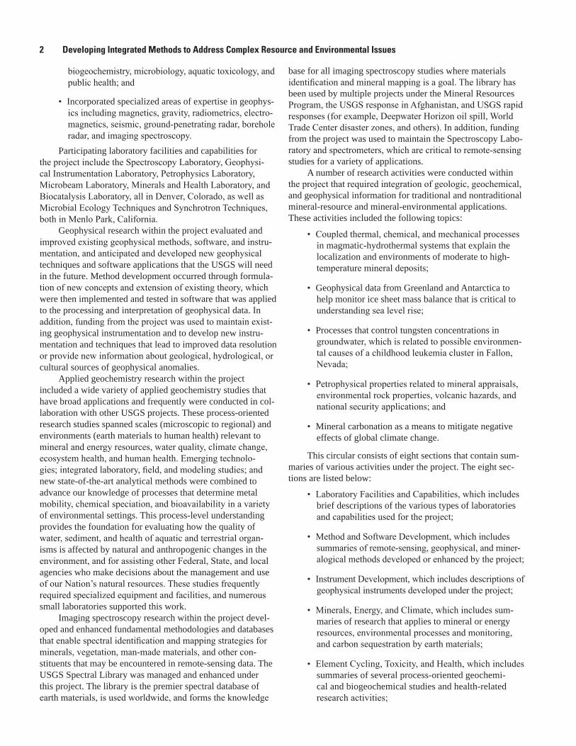
2 Developing Integrated Methods to Address Complex Resource and Environmental Issues
biogeochemistry, microbiology, aquatic toxicology, and public health; and
• Incorporated specialized areas of expertise in geophys-ics including magnetics, gravity, radiometrics, electro-magnetics, seismic, ground-penetrating radar, borehole radar, and imaging spectroscopy.
Participating laboratory facilities and capabilities for the project include the Spectroscopy Laboratory, Geophysi-cal Instrumentation Laboratory, Petrophysics Laboratory, Microbeam Laboratory, Minerals and Health Laboratory, and Biocatalysis Laboratory, all in Denver, Colorado, as well as Microbial Ecology Techniques and Synchrotron Techniques, both in Menlo Park, California.
Geophysical research within the project evaluated and improved existing geophysical methods, software, and instru-mentation, and anticipated and developed new geophysical techniques and software applications that the USGS will need in the future. Method development occurred through formula-tion of new concepts and extension of existing theory, which were then implemented and tested in software that was applied to the processing and interpretation of geophysical data. In addition, funding from the project was used to maintain exist-ing geophysical instrumentation and to develop new instru-mentation and techniques that lead to improved data resolution or provide new information about geological, hydrological, or cultural sources of geophysical anomalies.
Applied geochemistry research within the project included a wide variety of applied geochemistry studies that have broad applications and frequently were conducted in col-laboration with other USGS projects. These process-oriented research studies spanned scales (microscopic to regional) and environments (earth materials to human health) relevant to mineral and energy resources, water quality, climate change, ecosystem health, and human health. Emerging technolo-gies; integrated laboratory, field, and modeling studies; and new state-of-the-art analytical methods were combined to advance our knowledge of processes that determine metal mobility, chemical speciation, and bioavailability in a variety of environmental settings. This process-level understanding provides the foundation for evaluating how the quality of water, sediment, and health of aquatic and terrestrial organ-isms is affected by natural and anthropogenic changes in the environment, and for assisting other Federal, State, and local agencies who make decisions about the management and use of our Nation’s natural resources. These studies frequently required specialized equipment and facilities, and numerous small laboratories supported this work.
Imaging spectroscopy research within the project devel-oped and enhanced fundamental methodologies and databases that enable spectral identification and mapping strategies for minerals, vegetation, man-made materials, and other con-stituents that may be encountered in remote-sensing data. The USGS Spectral Library was managed and enhanced under this project. The library is the premier spectral database of earth materials, is used worldwide, and forms the knowledge
base for all imaging spectroscopy studies where materials identification and mineral mapping is a goal. The library has been used by multiple projects under the Mineral Resources Program, the USGS response in Afghanistan, and USGS rapid responses (for example, Deepwater Horizon oil spill, World Trade Center disaster zones, and others). In addition, funding from the project was used to maintain the Spectroscopy Labo-ratory and spectrometers, which are critical to remote-sensing studies for a variety of applications.
A number of research activities were conducted within the project that required integration of geologic, geochemical, and geophysical information for traditional and nontraditional mineral-resource and mineral-environmental applications. These activities included the following topics:
• Coupled thermal, chemical, and mechanical processes in magmatic-hydrothermal systems that explain the localization and environments of moderate to high-temperature mineral deposits;
• Geophysical data from Greenland and Antarctica to help monitor ice sheet mass balance that is critical to understanding sea level rise;
• Processes that control tungsten concentrations in groundwater, which is related to possible environmen-tal causes of a childhood leukemia cluster in Fallon, Nevada;
• Petrophysical properties related to mineral appraisals, environmental rock properties, volcanic hazards, and national security applications; and
• Mineral carbonation as a means to mitigate negative effects of global climate change.
This circular consists of eight sections that contain sum-maries of various activities under the project. The eight sec-tions are listed below:
• Laboratory Facilities and Capabilities, which includes brief descriptions of the various types of laboratories and capabilities used for the project;
• Method and Software Development, which includes summaries of remote-sensing, geophysical, and miner-alogical methods developed or enhanced by the project;
• Instrument Development, which includes descriptions of geophysical instruments developed under the project;
• Minerals, Energy, and Climate, which includes sum-maries of research that applies to mineral or energy resources, environmental processes and monitoring, and carbon sequestration by earth materials;
• Element Cycling, Toxicity, and Health, which includes summaries of several process-oriented geochemi-cal and biogeochemical studies and health-related research activities;

Introduction 3
• Hydrogeology and Water Quality, which includes descriptions of innovative geophysical, remote-sensing, and geochemical research pertaining to hydro-geology and water-quality applications;
• Hazards and Disaster Assessment, which includes sum-maries of research and method development that were applied to natural hazards, human-caused hazards, and disaster assessments; and
• Databases and Framework Studies, which includes descriptions of fundamental applications of geophysi-cal studies and of the importance of archived data.

Spectroscopy Laboratory
By Gregg A. Swayze
The U.S. Geological Survey (USGS) Denver, Colorado, Spectroscopy Laboratory houses analytical instruments for the spectral measurement of samples under a full range of pressure and temperature conditions necessary to mimic all extremes on the Earth’s surface and the moons of the outer planets (fig. 2). Capabilities include reflectance and trans-mission measurements from the ultraviolet out into the far infrared (0.1 to 150 micrometers) at temperatures ranging
from 77 to 500 kelvin (K) (–320 to 440 degrees Fahrenheit [°F]) and pressures ranging from a total vacuum up to several atmospheres. Data collected on these spectrometers have been used to map water on the Moon (Clark and others, 2009), identify opal on Mars (Milliken and others, 2008), and create an online spectral library used worldwide (Clark and others, 2007). It is likely that the Denver Spectroscopy Laboratory is the only lab capable of making spectral measurements that span such a wide range of environmental conditions. We can bring our visible/near-infrared spectrometers to the field to make in situ measurements of samples and calibrate broad-band or hyperspectral remote-sensing data. In the past, these portable instruments have played a critical role in mapping
Figure 2. This analytical instrument has a specially designed environment chamber for spectral measurement of materials over a wide range of temperatures and pressures at wavelengths from the ultraviolet to the far infrared. This equipment allows simulation of conditions at the outer planets and extremes on the Earth’s surface. Multiple observation ports allow measurement by several spectrometers without disturbing the samples. (USGS photograph)
Laboratory Facilities and Capabilities

Laboratory Facilities and Capabilities 5
acid-mine drainage at abandoned mines (Swayze and others, 2000), measuring asbestos in the World Trade Center dust (Clark and others, 2001) and potentially asbestos-bearing rocks in communities in the Sierra Nevada Foothills (Swayze and others, 2009), characterizing vegetation biochemistry to monitor global change (Kokaly and Clark, 1999), examining highly alkaline ash from wildfires (Kokaly and others, 2008), providing calibration for hyperspectral mineral images of Afghanistan (Kokaly and others, 2011), and estimating the volume of oil floating on the ocean surface during the Deep-water Horizon oil spill (Clark and others, 2010).
To support these endeavors, the lab houses several mineral collections with thousands of samples used to com-pile our online spectral library used throughout the world by scientists conducting laboratory and remote-sensing studies. One of the collections contains man-made building materi-als so their spectra can be used to accurately map urban areas in case of natural or man-made disasters. We continually add new mineral entries to the library collections to support new remote-sensing applications. One thing that sets our spectral library apart from others is that we analyze sample purity with multiple analytical techniques and include this “metadata” with the spectra in our online library.
A key part of the Spectroscopy Laboratory is its com-puting facilities, which are some of the largest in the USGS. Spectroscopic analysis and hyperspectral mapping and iden-tification require tremendous computing power. The USGS Spectroscopy Laboratory has multiple Linux and UNIX com-puter servers. The main machine is a 24-cpu (central process-ing unit) system with 296 gigabytes of random access memory (RAM) and more than 140 terabytes of disk space, containing spectroscopy and hyperspectral data for the Earth, Mars, the Moon, and other objects throughout the Solar System. The compute power allows up to 60 million spectral features per second to be compared enabling large imaging spectroscopy datasets to be analyzed rapidly.
References Cited
Clark, R.N., 2009, Detection of absorbed water and hydroxyl on the Moon: Science, v. 226, no. 5952, p. 562–564.
Clark, R.N., Green, R.O., Swayze, G.A., Meeker, Greg, Sutley, Steve., Hoefen, T.M., Livo, K.E., Plumlee, Geoff, Pavri, Betina, Sarture, Chuck, Wilson, Steve, Hageman, Phil, Lamothe, Paul, Vance, J.S., Boardman, Joe, Brown-field, Isabelle, Gent, Carol, Morath, L.C., Taggart, Joseph, Theodorakos, P.M., and Adams, Monique, 2001, Environ-mental studies of the World Trade Center area after the Sep-tember 11, 2001 attack: U.S. Geological Survey Open-File Report 01–0429, 260 p.
Clark, R.N., Swayze, G.A., Leifer, Ira, Livo, K.E., Kokaly, Raymond, Hoefen, Todd, Lundeen, Sarah, Eastwood, Michael, Green, R.O., Pearson, Neil, Sarture, Charles, McCubbin, Ian, Roberts, Dar, Bradley, Eliza, Steele, Denis, Ryan, Thomas, Dominguez, Roseanne, and the Airborne Visible/Infrared Imaging Spectrometer (AVIRIS) Team, 2010, A method for quantitative mapping of thick oil spills using imaging spectroscopy: U.S. Geological Survey Open-File Report 2010–1167, 51 p.
Clark, R.N., Swayze, G.A., Wise, R.A., Livo, K.E., Hoefen, T.M., Kokaly, R.F., and Sutley, S.J., 2007, USGS digital spectral library splib06a: U.S. Geological Survey Digital Data Series DS–231, [about 6,100] p.
Kokaly, R.F., and Clark, R.N., 1999, Spectroscopic determi-nation of leaf biochemistry using band-depth analysis of absorption features and stepwise multiple linear regression: Remote Sensing of Environment, v. 67, p. 267–287.
Kokaly, R.F., King, T.V.V., Hoefen, T.M., Dudek, K.B., and Livo, K.E., 2011, Surface materials map of Afghanistan—Carbonates, phyllosilicates, sulfates, altered minerals, and other materials: U.S. Geological Survey Scientific Investi-gations Map 3152–A, one sheet, scale 1:1,100,000, http://pubs.usgs.gov/sim/3152/A/.
Kokaly, R.F., Rockwell, B.W., Haire, S.L., and King, T.V.V., 2007, Characterization of post-fire surface cover, soils, and burn severity at the Cerro Grande Fire, New Mexico, using hyperspectral and multispectral remote sensing: Remote Sensing of Environment, v. 106, p. 305–325.
Milliken, R.E., Swayze, G.A., Arvidson, R.E., Bishop, J.L., Clark, R.N., Ehlmann, B.L., Green, R.O., Grotzinger, J.P., Morris, R.V., Murchie, S.L., Mustard, J.F., Weitz, C., and the CRISM Science Team, 2008, Opaline silica in young deposits on Mars: Geology, v. 36, no. 11, p. 847–850.
Swayze, G.A., Kokaly, R.F., Higgins, C.T., Clinkenbeard, J.P., Clark, R.N., Lowers, H.A., and Sutley, S.J., 2009, mapping potentially asbestos-bearing rocks using imaging spectros-copy: Geology, v. 37, no. 8, p. 763–766.
Swayze, G.A., Smith, K.S., Clark, R.N., Sutley, S.J., Pearson, R.N., Rust, G.S., Vance, J.S., Hageman, P.L., Briggs, P.H., Meier, A.L., Singleton, M.J., and Roth, Shelly, 2000, Using imaging spectroscopy to map acidic mine waste: Environ-mental Science and Technology, v. 34, no. 1, p. 47–54.

6 Developing Integrated Methods to Address Complex Resource and Environmental Issues
Geophysical Instrumentation Laboratory
By Craig W. Moulton
The primary objective of the Geophysical Instrumenta-tion Laboratory is the development of new geophysical instru-mentation that will lead to improved data resolution or provide other new information about geological, hydrological, or cul-tural sources of geophysical anomalies. A secondary objective is the maintenance of existing geophysical instrumentation.
The laboratory has a full machine shop containing two large engine lathes, two large mills and all associated tool-ing, large-throat band saws, a wide metal shear and brake, full welding capability (inert gases/arc/brazing/plasma cutter/oxyacetylene), bead blasting, grinders, and band sanders. Also available is a full woodshop containing saws (radial/table/compound miter/scroll/band), a joiner, drill press, and router table. The electronic laboratory equipment consists of oscil-loscopes, function generators, network analyzers, laboratory power supplies, data acquisition systems, and a large assort-ment of board-level electronic components. The laboratory has printed circuit board layout capability. Software is developed
for controlling data acquisition systems using the LabVIEW (from National Instruments) programming language.
Leveraging funding from the U.S. Department of Defense Strategic Environmental Research and Development Program and the Environmental Technology Demonstration and Valida-tion Program, the laboratory has developed a tractor-towed unexploded ordnance (UXO) detection system called the ALLTEM (on ALL the Time Electro-Magnetic) (fig. 3). The laboratory contributed its expertise in the development and fabrication of the ALLTEM mechanical systems (fiberglass cart and detection cube) and the electronic control and data acquisi-tion systems. Software was developed to use global positioning system information to aid in UXO survey planning and trac-tor steering accuracy. The ALLTEM system is currently being used at a UXO cleanup project in Texas. Other projects recently developed include a seismic hammer-strike sensor with wireless transmission to a data acquisition system, an automated antenna positioning system to perform cross-well radar tomography experiments in a large sand tank, fabrication of flux-gate mag-netometer instruments used for in situ long-term monitoring, and a modernization (new software and hardware) of the U.S. Geological Survey Petrophysics Instrumentation Laboratory’s nonlinear complex-resistivity measurement system.
Figure 3. Geophysical Instrumentation Laboratory projects and facilities. A, ALLTEM (on ALL the Time Electro-Magnetic) system performing an unexploded ordnance survey; B, ALLTEM cube; C, Machine shop; D, Magnetometer; and E, Wireless hammer. (USGS photographs)
A B
C ED

Laboratory Facilities and Capabilities 7
Denver Microbeam Laboratory for Microanalysis
By Heather A. Lowers
The Denver Microbeam Laboratory is an analytical facility that specializes in microanalysis—both chemical and morphological—of rocks, minerals, dust and particulates, and other materials from a wide variety of applications using electron-beam-based techniques. The laboratory supports programs within the Energy and Minerals and Environmental Health Mission Areas as well as other mission areas within the U.S. Geological Survey (USGS). In addition to collabo-rating with, and providing microanalytical services to USGS researchers, the Denver Microbeam Laboratory caters to a number of Federal, State, and international agencies, and aca-demic researchers by agreement.
The Denver Microbeam Laboratory operates low-vacuum, low-voltage scanning electron microscopes (SEM). They are equipped with energy dispersive (EDS) X-ray analysis sys-tems that are capable of elemental detection from beryllium to uranium. The EDS system provides the capability to image and chemically analyze a variety of samples including biologi-cal and geological materials, ceramics, polymers, compos-ites, and metals. Both instruments are capable of imaging, at nanometer resolution, the surface features of materials (sec-ondary electron imaging), subtle density variations within a sample (backscattered electron imaging), as well as defects related to trace-element impurities and structural defects (cathodoluminescence). One SEM is also equipped with an electron backscatter diffraction system that provides crystal structural information of the material. In addition there is a fully automated electron microprobe (electron probe micro-analyzer, EPMA) designed to produce in situ, quantitative elemental analysis from sample volumes as small as 2 micrometer in diameter at better than two percent accuracy and precision. The detection limit for most elements is between 300–800 parts per million, but using advanced methods, detection limits can be at single-digit parts per million levels. The electron microprobe also offers wavelength-dispersive X-ray intensity mapping, which provides better energy resolution than EDS mapping.
The Denver Microbeam Laboratory also maintains stereo and petrographic transmitted- and reflected-light microscopes with digital imaging capability and a variety of image pro-cessing and desktop publishing software. The laboratory has a clean room and facilities for manipulating small particles in preparation for analysis. Sample preparation equipment includes a vacuum impregnator, mechanical polishing appara-tus, and an ion mill.
Selection of Published Research Supported by the Denver Microbeam Laboratory
Aleinikoff, J.N., Creaser, R.A., Lowers, H.A., Magee, C.W., Jr., and Grauch, R.I., 2012, Multiple age components in individual molybdenite grains: Chemical Geology, v. 300–301, p. 55–60.
Diehl, S.F., Goldhaber, M.B., Lowers, H.A., Koenig, A.E., and Ruppert, L.F., 2012, Distribution of arsenic, selenium, and other trace elements in high pyrite Appalachian coals—Evidence for multiple episodes of pyrite formation: Interna-tional Journal of Coal Geology Special Issue, Minerals and Trace Elements in Coal, v. 94, p. 238–249.
Fishman, N.S., Hackley, P.C., Lowers, H.A., Hill, R.J., Egen-hoff, S.O., Eberl, D.D., and Blum, A.E., 2012, The nature of porosity in organic-rich mudstones of the Upper Jurassic Kimmeridge Clay Formation, North Sea, offshore United Kingdom: International Journal of Coal Geology, v. 103, p. 32–50.
Henley, R.W., and Berger, B.R., 2012, Pyrite-sulfosalt reac-tions and semimetal fractionation in the Chinkuashih, Taiwan, copper-gold deposit—A 1 Ma paleo-fumarole: Geofluids, v. 12, p. 245–260.
Lowers, H.A., Breit, G.N., Foster, A.L., Whitney, John, Yount, James, Uddin, Md. Nehal, and Muneem, Ad. Atual, 2007, Arsenic incorporation into authigenic pyrite, Bengal Basin sediment, Bangladesh: Geochimica et Cosmochimica Acta, v. 71, p. 2699–2717.
Lowers, H.A., Meeker, G.P., Lioy, P.J., and Lippmann, Mor-ton, 2009, Summary of the development of a signature for detection of residual dust from collapse of the World Trade Center buildings: Journal of Exposure Science and Environ-mental Epidemiology, v. 19, p. 325–335.
Rusk, B.G., Lowers, H.A., and Reed, M.H., 2008, Trace elements in hydrothermal quartz—Relationships to cath-odoluminescent textures and insights into vein formation: Geology, v. 36, no. 7, p. 547–550.
Wilson, S.A., Koenig, A.E., and Lowers, H.A, 2012, A new basaltic glass microanalytical reference material for mul-tiple techniques: Microscopy Today, v. 20, p. 12–16.

8 Developing Integrated Methods to Address Complex Resource and Environmental Issues
Minerals and Health Laboratory
By Suzette A. Morman
Earth scientists have a growing role in understanding and anticipating potential health issues associated with toxic metal(loid)s in often poorly understood earth materials such as dust, volcanic ash, wildfire ash, and mine wastes. By eluci-dating the mineralogical and geochemical characteristics of these materials, earth scientists can aid in identifying primary exposure pathways of concern, how materials may be taken up by the body, and the chemical behavior and toxicological properties of the materials once in the body. Through the use of laboratory methods such as physiologically based extraction tests, our Minerals and Health Laboratory provides valuable information on the solubility or bioaccessibility of elements present in earth materials.
Bioaccessibility, generally defined as the amount of a metal(loid) that is soluble in a simulated gastric solution, provides an estimate of what is available to the body for uptake (Ruby and others, 1999). Although it does not measure bioavailability (what is actually taken up by target organs such as the kidneys or liver), bioaccessibility provides a quick and inexpensive alternative to animal testing studies that directly measure uptake of toxicants from earth materials. This testing methodology is frequently used in Europe as well as in the United States (Oomen and others, 2002). The Minerals and Health Laboratory has used and modified physiologically based extraction tests (PBET), also called in vitro bioacces-sibility (IVBA) tests, to examine the bioaccessibility of metal/metalloid toxicants in a variety of earth materials and sample-medium types. Our gastric bioaccessibility method is based on a U.S. Environmental Protection Agency (EPA) method to evaluate the bioaccessibility of lead (EPA, 2008). We also test potential bioaccessibility of inhaled or respired earth materi-als using simulated lung fluids (Morman and others, 2013), serum-based fluids, and fluids simulating those found in cells that engulf and digest foreign particles in the lungs and upper respiratory tract.
Projects
The following U.S. Geological Survey projects and groups have utilized the capabilities of the Minerals and Health Laboratory:
• Effects of Climatic Variability and Land Use on Ameri-can Drylands,
• Geoanalytical Research Chemistry Group, and
• U.S. Geological Survey Reference Materials and Min-erals and Health.
Primary Products
The following reports, from latest to earliest, utilized results from the Minerals and Health Laboratory:Goldstein, H.L., Reynolds, R.L., Morman, S.A., Moskowitz,
Bruce, Kokaly, R.F., Goossens, Dirk, Buck, B.J., Flagg, Cody, Till, Jessica, Yauk, Kimberly, and Berquó, T.S., 2013, Iron mineralogy and bioaccessibility of dust generated from soils as determined by reflectance spectroscopy and magnetic and chemical properties—Nellis Dunes recre-ational area, Nevada: U.S. Geological Survey Scientific Investigations Report 2013–5054, 15 p. http://pubs.usgs.gov/sir/2013/5054/.
Plumlee, G.S., Durant, J.T., Morman, S.A., Neri, Antonio, Wolf, R.E., Dooyema, C.A., Hageman, P.L., Lowers, H.A., Fernette, G.L., Meeker, G.P., Benzel, W.M., Driscoll, R.L., Berry, C.J., Crock, J.G., Goldstein, H.L., Adams, Monique, Bartrem, C.L., Tirima, Simba, Behbod, BBehrooz, von Lindern, IIan, and Brown, M.J., 2013, Linking geological and health sciences to assess childhood lead poisoning from artisanal gold mining in Nigeria: Environmental Health Perspectives, v. 121, no.6, p. 744–750.
Morman, Suzette, 2012, In vitro bioavailability extractions, Appendix E, in Driscoll, Rhonda, Hageman, P.L., Benzel, W.M., Diehl, S.F., Adams, D.T., Morman, Suzette, and Cho-ate, L.M., Assessment of the Geoavailability of Trace Ele-ments from Minerals in Mine Wastes: Analytical Techniques and Assessment of Selected Copper Minerals: U.S. Geo-logical Survey Scientific Investigations Report 2011–5211, p. 34–43. http://pubs.usgs.gov/sir/2011/5211/.
Wolf, R.E., Morman, S.A., Hageman, P.L, Hoefen, T.M., and Plumlee, G.S., 2011, Simultaneous speciation of arsenic, selenium, and chromium: species stability, sample preserva-tion, and analysis of ash and soil leachates: Analytical and Bioanalytical Chemistry, v. 401, no. 9, p. 2733–2745. doi: 10.1007/s00216-011-5275-x.
Gray, J.E., Plumlee, G.S., Morman S.A., Higueras, P.L., Crock, J.G., Lowers, H.A., and Witten, M.L., 2010, In vitro studies evaluating leaching of mercury from mine waste calcine using simulated human body fluids: Environmental Science and Technology, v. 44, no. 12, p. 4782–4788. doi: 10.1021/es1001133.
Garrison, Virginia, Lamothe, Paul, Morman, Suzette, and Plumlee, Geoffrey, 2010, Trace-metal concentrations in African dust: Effects of long-distance transport and implica-tions for human health: 19th World Congress of Soil Sci-ence, August1–6, 2010, Brisbane, Australia.
Morman, S.A., 2010, Arsenic: A detective story in dusts: Earth Magazine, v. 55, no. 6, p. 40–47.

Laboratory Facilities and Capabilities 9
References Cited
Morman, S.A., Garrison, V.H., and Plumlee, G.S., 2013, Trace metals in Saharan dust: The use of in vitro bioaccessibil-ity extractions to assess potential health risks in a dustier world: American Chemical Society Symposium Series 1149, p. 41–58.
Oomen, A.G., Hack, Alfons, Minekus, Mans, Zeijdner, Evelijn, Cornelis, Christa, Schoeters, Greet, Verstraete, Willy, Van de Wiele, Tom, Wragg, Joanna, Rompelberg, C.J.M., Sips, A.J.A.M., and Van Wijnen, J.H., 2002, Com-parison of five in vitro digestion models to study the bioac-cessibility of soil contaminants: Environmental Science & Technology, v. 36, p. 3326–3334.
Ruby, M.V., Schoof, R., Brattin, W., Goldade, M., Post, G., Harnois, M., Mosby, D.E., Casteel, S.W., Berti, W., Carpen-ter, M., Edwards, D., Cragin, D., and Chappell, W., 1999, Advances in evaluating the oral bioavailability of inorganics in soil for use in human health risk assessment: Environ-mental Science & Technology, v. 33, p. 3697–3705.
U.S. Environmental Protection Agency (EPA), 2008, Standard operating procedure for an in vitro bioaccessibility assay for lead in soil: U.S. Environmental Protection Agency, EPA 9200.2-86, 9 p., http://nepis.epa.gov/.
Petrophysics LaboratoryBy Robert J. Horton
The Petrophysics Laboratory (PetLab) has the ability to measure the physical properties of earth materials (fig. 4). Knowledge of physical properties is essential in the interpreta-tion of geophysical data, for survey design, numerical model-ing, and geophysical sensor development. PetLab measure-ments can determine the density and magnetic, electrical, and radioactive properties of solid rocks, unconsolidated sedi-ments, and liquids. Laboratory measurements show the range of physical properties to be expected for a given geologic unit or site and can show how those properties change as condi-tions vary. For example, the electrical properties of the ground vary as a function of water content, which can be manipulated in the laboratory to represent different conditions. By combin-ing physical property measurements with geochemical and mineralogical data, an integrated interpretation can be made showing the effect of the composition of a sample on its geo-physical signature (that is, McCafferty and others, 2011).
References Cited
McCafferty, A.E., Horton, R.J., Stanton, M.R., McDougal, R.R., and Fey, D.L., 2011, Geophysical geochemical, mineralogical, and environmental data for rock samples col-lected in a mineralized volcanic environment, upper Animas River watershed, Colorado: U.S. Geological Survey Data Series 595, 13 p.
Figure 4. Sediment sample prepared for a four-electrode, low-frequency (0.001 to 1,000 hertz) electrical resistivity measurement. (USGS photograph)
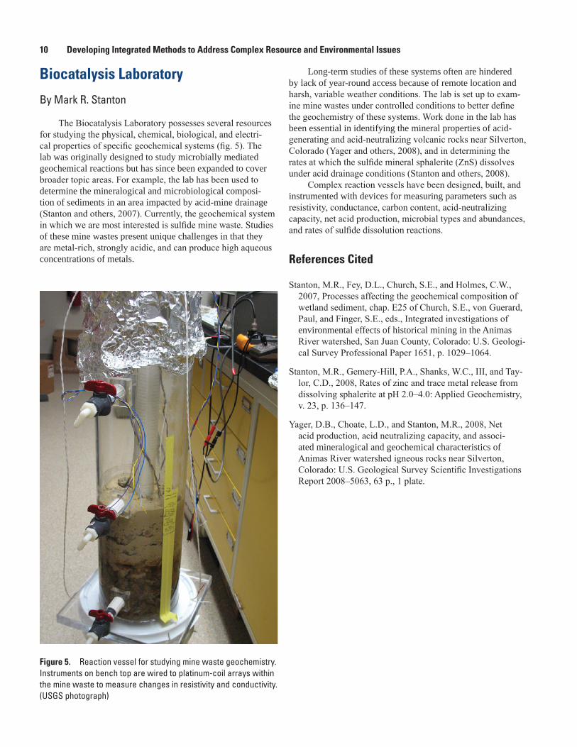
10 Developing Integrated Methods to Address Complex Resource and Environmental Issues
Biocatalysis Laboratory
By Mark R. Stanton
The Biocatalysis Laboratory possesses several resources for studying the physical, chemical, biological, and electri-cal properties of specific geochemical systems (fig. 5). The lab was originally designed to study microbially mediated geochemical reactions but has since been expanded to cover broader topic areas. For example, the lab has been used to determine the mineralogical and microbiological composi-tion of sediments in an area impacted by acid-mine drainage (Stanton and others, 2007). Currently, the geochemical system in which we are most interested is sulfide mine waste. Studies of these mine wastes present unique challenges in that they are metal-rich, strongly acidic, and can produce high aqueous concentrations of metals.
Long-term studies of these systems often are hindered by lack of year-round access because of remote location and harsh, variable weather conditions. The lab is set up to exam-ine mine wastes under controlled conditions to better define the geochemistry of these systems. Work done in the lab has been essential in identifying the mineral properties of acid-generating and acid-neutralizing volcanic rocks near Silverton, Colorado (Yager and others, 2008), and in determining the rates at which the sulfide mineral sphalerite (ZnS) dissolves under acid drainage conditions (Stanton and others, 2008).
Complex reaction vessels have been designed, built, and instrumented with devices for measuring parameters such as resistivity, conductance, carbon content, acid-neutralizing capacity, net acid production, microbial types and abundances, and rates of sulfide dissolution reactions.
References Cited
Stanton, M.R., Fey, D.L., Church, S.E., and Holmes, C.W., 2007, Processes affecting the geochemical composition of wetland sediment, chap. E25 of Church, S.E., von Guerard, Paul, and Finger, S.E., eds., Integrated investigations of environmental effects of historical mining in the Animas River watershed, San Juan County, Colorado: U.S. Geologi-cal Survey Professional Paper 1651, p. 1029–1064.
Stanton, M.R., Gemery-Hill, P.A., Shanks, W.C., III, and Tay-lor, C.D., 2008, Rates of zinc and trace metal release from dissolving sphalerite at pH 2.0–4.0: Applied Geochemistry, v. 23, p. 136–147.
Yager, D.B., Choate, L.D., and Stanton, M.R., 2008, Net acid production, acid neutralizing capacity, and associ-ated mineralogical and geochemical characteristics of Animas River watershed igneous rocks near Silverton, Colorado: U.S. Geological Survey Scientific Investigations Report 2008–5063, 63 p., 1 plate.
Figure 5. Reaction vessel for studying mine waste geochemistry. Instruments on bench top are wired to platinum-coil arrays within the mine waste to measure changes in resistivity and conductivity. (USGS photograph)

Laboratory Facilities and Capabilities 11
Gene-Based Techniques in Support of U.S. Geological Survey Environmental Health and Ecology Studies
By Andrea L. Foster
During the past ≈30 years, scientific interest in the role microorganisms play in controlling the major forms (for example, valence-state) of elements (their speciation) on Earth has increased dramatically to become a major subdiscipline, often called “geomicrobiology.” In the area of geochemistry, many water-mineral reactions critical to the cycling of trace elements are recognized to be microbially driven, including the oxidative dissolution and reductive formation of pyrite and the reductive dissolution/oxidative precipitation of iron and manganese oxides (for example, Tebo, 1997). Microbes that use toxic trace elements in their metabolic cycle (for example, arsenic-reducing bacteria) clearly also play important roles in the mobility of those elements, especially with regard to water quality in potable groundwater supplies (Sutton and others, 2009). The role of microbes in the cycling of carbon (fixing in carbonate minerals and mobilizing via respiration) and nitrogen is also a subject of great interest (Harms and Grimm, 2008). The isolation of individual microbes from the envi-ronment and characterization of their physiology, as well as measurement of in situ turnover rates by unidentified micro-bial communities (that is, sulfur reduction), has allowed geo-chemists to develop quantitative values for the rates at which microbes perform geochemical reactions. These rates are then added to geochemical models used to describe and (or) predict the behavior of elements such as carbon (after below-ground sequestration or in warming, Alaskan peat deposits), arsenic, chromium, mercury, and uranium (in naturally or anthropo-genically contaminated aquifer sediment) (Bethke, 2008).
Although these approaches continue to be valuable to geomicrobiologists, it is also well-recognized that isolation approaches only provide the equivalent of a fleeting glimpse into the microbial world and its great diversity. It has been estimated that less than 1 percent of the microbes in the environment can be cultivated. Gene-based studies provide a wider window into the microbial world of the natural environ-ment because their starting material (nucleic acid) is extracted directly from microbes. Two main goals of gene-based studies have been the identification and quantification of microbial groups. Studies tracking these variables across environmental gradients (salinity, temperature, water, oxygen concentration, and contamination) and time have been conducted in support of projects within the Energy, Minerals, and Environmental Health Mission Area. With these data, ecological principles can be applied to improve process-based understanding and descriptive/predictive modeling of microbial population dynamics at sites where that information is of substantial value to the Nation.
Below is a brief summary of gene-based techniques for which method development was supported by the
Integrated Methods Development Project, with examples of how these developments have supported various USGS projects. It is important to note that this summary is quite limited in scope and is not an attempt to describe all the available gene-based techniques.
A major research thrust has been toward the develop-ment of high-throughput methods that allow capture of significantly larger amounts of gene-based data from the environment. Automation and miniaturization of processes have been important in this regard, as has been substitut-ing gel-based procedures for liquid-based ones. The primary activity supported under the project was the development of high-throughput chromatographic procedures for the size- and sequence-dependent separation of DNA (deoxyribonucleic acid) fragments to replace gel-based methods, which are more tedious and have larger errors related to the extracted data.
Polymerase chain reaction (PCR) is a standard tech-nique for the amplification of specific DNA fragments. DNA extracted from an environmental sample such as pond mud, groundwater, soil, or biological secretion is a mix of prokary-otic and eukaryotic DNA, as well as protein and other unde-sirable contaminants. PCR employs primers (short pieces of single-stranded DNA) to ensure that only specific regions of the genome are amplified. Primers are chosen from the litera-ture (or developed by the user) and can be very general or very specific (down to strains of E. coli, for example). The ampli-fication is conducted under a series of precisely controlled thermal cycles producing an exponential copy rate. PCR is used for detection of low-abundance species of concern (that is, specific pathogens) but is also the workhorse genetic tech-nique producing the amplified DNA required for downstream techniques such as gel electrophoresis, DNA chromatography, and DNA sequencing.
Under the Integrated Methods Development, PCR meth-ods were optimized for use of the reaction products in DNA chromatography (see below). Numerous common additives in PCR reactions cannot be put through the chromatographic column, so the use of alternative thermal-cycle methods to produce high-yield and specific PCR reactions were investi-gated and best methods developed.
Quantitative PCR (qPCR) is a related technique that offers additional benefits; primary among these benefits is that the amount of amplified DNA at each cycle of the PCR can be quantified and used to determine the amount of the specific gene fragment that was present prior to the amplifica-tion. QPCR has been used to track the relative abundances of microbial populations at the kingdom (for example, Eubac-teria, Archea, and Eukaryotes), group (for example, sulfate reducers), and subspecies (for example, E. coli strains) levels. Under the project, published qPCR methods were tested and run on samples relevant to projects concerning the extent of microbial methylation of mercury, microbial sequestration and transformation of arsenic in a former gold mine, and microbial populations in intertidal sediments impacted by mining of vol-canic massive sulfide deposits. These data are being compiled for future reports.

12 Developing Integrated Methods to Address Complex Resource and Environmental Issues
Polyacrylamide gel electrophoresis (PAGE) and dena-turing gradient gel electrophoresis (DGGE) are vertical, thin (1–2 millimeter thick), acrylamide gel techniques used to analyze PCR products based on size (PAGE) or sequence (DGGE). Both techniques use an applied electric field to propel DNA fragments through the small holes in the gel—in PAGE, the gel is pure acrylamide, but for DGGE, the gel also contains a denaturing agent that forces the double-stranded DNA to separate and migrate at a rate that is effectively sequence-dependent. Gels can be imaged and converted to digital data, which can be analyzed by multivariate statistical techniques, but gels are inherently difficult to reproduce and have large quantification error. Individual bands can also be cut out of gels, and the sequence within that band determined and used to help identify the organism. Under the project, PAGE and DGGE gels of PCR-amplified DNA fragments were run primarily as a comparison with DNA chromato-graphic techniques that were the main focus of the project.
DNA chromatography is analogous to PAGE/DGGE but uses reversed-phase ion-paring chromatography to separate PCR-amplified DNA fragments on the basis of sequence or size. DNA chromatography is more sensitive to PCR reac-tion chemistry than PAGE/DGGE but is more quantifiable, reproducible, and automated. Furthermore, the separated DNA fragments can be recovered by automated fraction collection for downstream cloning, sequencing, or other pur-poses. Automation of sample injection and fraction collection increases the throughput and decreases the time necessary to obtain information about the diversity and composition of microbial communities. Data obtained in chromatogram format are, in principle, easier to analyze automatically and by standard multivariate statistical techniques than are gel-based data.
Under the project, published chromatographic methods for the analysis of microbial communities by DNA chroma-tography (Barlaan and others, 2005; Goldenberg and oth-ers, 2007) were applied to the projects listed above. Also, published methods for DGGE analysis of specific microbial groups, such as sulfate-reducing bacteria, were adapted for DNA chromatography and tested on samples related to the aforementioned projects. A large dataset was acquired for one project—a study of arsenic attenuation by iron-oxidizing microbes at a historic gold mine site (Foster and others, 2009)—and will be included in a later report. Findings to date indicate that the population is dominated by members of the genus Leptothrix, which are peculiar in their ability to pre-cipitate large amounts of carbon-based “sheaths” that become coated with iron- and manganese-oxide precipitates, which act as a sponge for arsenic (Foster and others, 2010). These communities may be effective in the removal of toxic arsenic from water as well as iron and manganese, which are problems in many rural water systems. In addition, carbon fixation is an added benefit that can be used in the total cost accounting of a bioremediation project.
References Cited
Barlaan, E.A., Sugimori, Miho, Furukawa, Seiji, and Takeu-chi, Kazuhisa, 2005, Profiling and monitoring of microbial populations by denaturing high-performance liquid chroma-tography: Journal of Microbiological Methods, v. 61, no. 3, p. 399–412.
Bethke, C.M., 2008, Geochemical and biogeochemical reac-tion modeling (2nd ed.): Cambridge University Press, 543 p.
Foster, A.L., Ashley, R.P., Ona-Nguema, Georges, Rytuba, J.J., and Brown, G.E., Jr., 2010, Microbially-mediated arsenic cycling at the Lava Cap Mine Superfund Site, Nevada County, CA [abs.]: Geological Society of America Abstracts with Program, v. 42, p. 500.
Foster, A.L., Ona-Nguema, Georges, Tufano, Kate, and White, Richard, III , 2009, Temporal chemical data for sediment, water, and biological samples from the Lava Cap Mine Superfund Site, Nevada County, California—2006–2008: U.S. Geological Survey Open-File Report 2009–1268, 46 p. http://pubs.usgs.gov/of/2009/1268/.
Goldenberg, Oliver, Herrmann, Stefanie, Marjoram, Gina, Noyer-Weidner, Mario, Hong, George, Bereswill, Stefan, and Gobel, U.B., 2007, Molecular monitoring of the intes-tinal flora by denaturing high performance liquid chroma-tography: Journal of Microbiological Methods, v. 68, no. 1, p. 94–105.
Harms, T.K., and Grimm, N.B., 2008, Hot spots and hot moments of carbon and nitrogen dynamics in a semiarid riparian zone: Journal of Geophysical Research G: Biogeo-sciences, v. 113, no. 1, p. 1–14.
Sutton, N.B., van der Kraan, G.M., van Loosdrecht, M.C.M., Muyzer, Gerard, Bruining, Johannes, and Schotting, R.J., 2009, Characterization of geochemical constituents and bac-terial populations associated with As mobilization in deep and shallow tube wells in Bangladesh: Water Research, v. 43, no. 6, p. 1720–1730.
Tebo, B.M., 1997, Bacterially-mediated mineral forma-tion—Insights into manganese(II) oxidation from molecular genetic and biochemical studies, in Banfield, J.F., and Neal-son, K.H., eds., Geomicrobiology—Interactions between microbes and minerals: Washington, D.C., Mineralogical Society of America, p. 225–260.

Laboratory Facilities and Capabilities 13
Identification of Trace-Metal Species and Their Distribution in Rocks, Sediments, and Biota Using Synchrotron Techniques
By Andrea L. Foster
Identification of the form in which an element occurs in the environment is as important as understanding the total amount that is present because an element’s form (also known as species) is an important determinant of its mobility in the environment and its toxicity. The X-ray-based tech-niques available at synchrotron light sources are being used to identify elemental species in rocks, sediments, and biota in situ, that is, with little or no preparation (Manceau and others, 2002). Most other techniques with the sensitivity required to measure trace elements in solids are ex situ, requiring manipu-lation of the sample by digestion, dissolution, drying, or other procedures in order to perform the analysis. These procedures often alter the original species distribution, confounding the analysis. In addition, significant quantities of sample (usually grams) are required for species measurement, but in some important cases, the important species are not easily sampled. The miniaturization of synchrotron X-ray beams (currently, most can be focused down to between 2 to 30 micrometers) has made the analysis of trace-element species in environmen-tal matrices at the micron scale possible.
Synchrotron-based X-ray fluorescence (XRF) mapping, X-ray diffraction (XRD), and X-ray absorption spectroscopy (XAS) are being employed more than ever before to under-stand trace-metal species in rocks, sediments, and biota in sup-port of USGS projects. The techniques involve illuminating a sample by a beam of ultrahigh-intensity X-rays (several orders of magnitude greater than that in a dentist’s office). XRF and XRD are two common instruments used in the conventional laboratory to extract chemical and mineralogical informa-tion (respectively) from bulk, powdered samples. Using the much higher flux of focused and tunable X-rays available at synchrotrons, element (and species) distribution maps with sensitivity on the parts per million (ppm) level can be pro-duced at micrometer scales under ambient conditions in moist or wet samples—something that would be impossible using conventional techniques. Similarly, benefits of conducting XRD analysis at the synchrotron include order-of-magnitude lower detection limits for trace crystalline phases and collec-tion of XRD patterns at the micrometer scale.
XAS analysis of elements at trace levels is a technique that is simply not feasible using laboratory X-ray sources. Analysis of XAS spectra provides information on an element’s valence state and molecular-scale coordination (number and distance of neighboring atoms) that is used to infer its specia-tion. In this experiment, high-energy X-rays (typically in the range of 7,000–30,000 electron volts for trace elements) are used to eject core-level electrons from a specific element of
interest in the sample. The scattering of these ejected electrons off of neighboring atoms produces modulations in the absor-bance spectrum that can be modeled quantitatively. The tech-nique has an operational detection limit of about 1–100 ppm, depending on the specific conditions of the experiment. As with XRF and XRD, XAS can be performed at the micrometer scale using focused synchrotron X-ray beams.
Through the project, several improvements in methods of synchrotron X-ray data collection and analysis were made. Investigations into alternative methods of cooling samples to improve the quality and quantity of data collection were performed. The performance of multivariate statistical analyses (particularly principal component analysis (PCA) on bulk XAS and micro-scale XRF/XAS datasets was tested on model datasets (Brown and others, 2010) and applied to USGS studies. Improvements in methods of collecting and analyzing synchrotron data have enhanced the quality of work produced by several USGS projects focused on aspects of (1) trace-element geochemistry (Foster and others, 2000; Foster and Ashley, 2002; Breit and others, 2004; Perkins and Foster, 2004; Lowers and others, 2007; Zielinski and others, 2007; Foster and others, 2010; Foster and others, 2011; Alp-ers and others, 2012), (2) the health of threatened ecosystems and characteristic megafauna (Foster and others, 2009), and (3) mineral resource studies of elements deemed critical to our Nation’s economy (A.L. Foster and others, oral com-mun., 2011; Hayes and others, 2011).
References Cited
Alpers, C.N., Burlak, T.L., Foster, A.L., Basta, N.T., and Mitchell, V.L., 2012, Arsenic and old gold mines—Mineralogy, speciation, and bioaccessibility [abs.]: V.M. Goldschmidt Conference, 22nd, Montreal, June 2012, p. 1418.
Breit, G.N., Foster, A.L., Perkins, R.B., Yount, J.C., King, Trude., Welch, A.H., Whitney, J.W., Uddin, M.N., Muneemn, A.A., and Alam, M.M., 2004, As-rich ferric oxy-hydroxide enrichments in the shallow subsurface of Ban-gladesh, in Wanty, R.B., and Seal, R.R., eds., Proceedings of the Eleventh International Symposium on Water-Rock Interaction: New York, A.A. Balkema, p. 1457–1461.
Brown, A.L., Foster, A.L., Alpers, C.N., Hansel, Colleen, Len-tini, Chris, and Kim, C.S., 2010, Factors affecting principal component analysis (PCA) of X-ray absorption fine struc-ture spectral datasets of arsenic and iron compounds [abs.]: Geological Society of America Abstracts with Program, v. 42, p. 615.
Foster, A.L., and Ashley, R.P., 2002, Characterization of arse-nic species in microbial mat communities in the vicinity of the Lava Cap gold mine, Nevada City, CA—Geochemistry: Exploration, Environment, and Analysis, v. 2, p. 253–261.

14 Developing Integrated Methods to Address Complex Resource and Environmental Issues
Foster, A.L., Ashley, R.P., Ona-Nguema, Georges, Rytuba, J.J., and Brown, G.E., Jr., 2010, Microbially-mediated arsenic cycling at the Lava Cap Mine Superfund Site, Nevada County, CA [abs.]: Geological Society of America Abstracts with Program, v. 42, p. 500.
Foster, A.L., Ashley, R.P., and Rytuba, J.J., 2011, Arsenic spe-cies in weathering mine tailings and biogenic solids at the Lava Cap Mine Superfund Site, Nevada City, CA: Geo-chemical Transactions, v. 12, no. 1, p. 1.
Foster, A.L., Berry, K., Jacobson, E.R., and Rytuba, J.J., 2009, Arsenic species in scute (shell plate) and lung tissue of desert tortoises: EOS Transactions American Geophysical Union Fall Meeting Supplement, v. 90, no. 52, p. B32B–04.
Foster, A.L., Breit, G.N., Welch, A.H., Whitney, J.W., Yount, J.C., Islam, M.S., Alam, M.M., Islam, M.K., and Islam, M.N., 2000, In-situ identification of arsenic species in soil and aquifer sediment from Ramrail, Brahmanbaria, Ban-gladesh [abs.]: American Geophysical Union Fall Meeting Supplement, p. H21D–01.
Hayes, S., Foster, A.L., and Balistrieri, L.S., 2011, Examin-ing tellurium geochemistry using laboratory-based sorption studies and spectroscopic investigation of natural samples [abs.]: American Geophysical Union Fall 2010 Meeting, Abstracts with Program, V13B–2598.
Lowers, H.A., Breit, G.N., Foster, A.L., Whitney, John, Yount, James, Uddin, M.N., and Muneem, A.A., 2007, Arsenic incorporation into authigenic pyrite, Bengal Basin sediment, Bangladesh: Geochimica et Cosmochimica Acta, v. 71, no. 11, p. 2699–2717.
Manceau, Alain, Marcus, M.A., and Tamura, Nobumichi, 2002, Quantitative speciation of heavy metals in soils and sediments by synchrotron X-ray techniques, in Fenter, P.A., Rivers, M.L., Sturchio, N.C., and Sutton, S.R., eds., Applications of synchrotron radiation in low-temperature geochemistry and environmental science: Washington, D.C., Mineralogical Society of America, p. 341–428.
Perkins, R.B., and Foster, A.L., 2004, Mineral affinities and distribution of selenium and other trace elements in black shale and phosphorite of the Phosphoria Formation, in Hein, J.R., ed., Life cycle of the Phosphoria Formation: New York, Elsevier, p. 251–298.
Zielinski, R.A., Foster, A.L., Meeker, G.P., and Brownfield, I.K., 2007, Mode of occurrence of arsenic in feed coal and its derivative fly ash, Black Warrior Basin, Alabama: Fuel, v. 86, p. 560–572.

Method and Software Development
U.S. Geological Survey Digital Spectral Library
By Roger N. Clark and Gregg A. Swayze
Issue and Scope
All analytical methods require standards and a knowledge base on which to verify results. Though traditional remote sensing can use simple ratios to show differences, imaging spectroscopy can detect, differentiate, and map subtle chemi-cal differences in minerals and other compounds. But to cor-rectly identify materials, their “spectral fingerprint” must be known. Without accurate knowledge of the spectral response of materials, accurate identification and mapping with spectro-scopic remote sensing would be impossible.
Spectroscopy is a tool that detects the absorption or emission of light. Our eyes are crude spectrometers: we see different colors in materials and can infer composition. For example, the green of chlorophyll absorbs blue and red light, leaving green, or the red in a rock is due to iron oxide that absorbs green and blue light. A digital camera is also a crude spectrometer, sensing three colors. Broad-band remote sensing instruments like Landsat Thematic Mapper have seven bands (colors) from the blue to infrared. But spectrometers contain more than 100 bands and can measure the detailed positions and shapes of absorption (or emission) bands in compounds (fig. 6). The absorptions observed in spectra of rocks, miner-als, and other compounds are due to chemical bonds, thus, “sense” the chemistry of the material, making it a very power-ful method that with current technology can be done from great distances. (Not to be confused with atomic emission spectroscopy, like the emission from a neon sign that “senses” atomic transitions.)
Objectives
The objective of the U.S. Geological Survey (USGS) spectral library is to provide reference spectra of minerals and other materials that could be encountered in nature and need to be distinguished in remote-sensing data. Materials include minerals, amorphous compounds, plants and other organic materials, man-made materials, environmental materials, and liquids that may be found in imaging spectroscopy datasets. The National Aeronautics and Space Administration (NASA) also funds spectroscopy of materials of planetary interest, and those spectra are also included in the spectral library.
Background
In order to interpret the vast array of absorptions seen in spectra of materials, we must know and understand those absorptions and how they change with subtle changes in chemistry. For example, a small substitution of an element in a mineral will change the length of chemical bonds in that mineral causing a shift in the absorption band position. Understanding that shift then enables one to remotely detect that substitution and map small changes in chemistry (see Clark and others, 1990; Clark, 1999; and Clark and others, 2003, 2007 for more details). The pyrite weathering sequence of spectra from the library shown in figure 7 illustrates the importance of spectral signatures. This sequence is key to identification and mapping of acidic rock drainage and led to a faster and lower cost cleanup of the Leadville, Colorado, min-ing district (Swayze and others, 2000).
Landsat TM
MODIS
AVIRISLaboratory
EXPLANATION
Low transmittance through Earth’s atmosphere
Wavelength, in micrometersRe
flect
ance
+ o
ffset
1
2
34
5
1.5
1.0
0.5
0.00.5 1.0 2.0 2.5 3.01.5
Figure 6. Comparison of spectra for alunite from four sensors with different spectral resolutions. Landsat Thematic Mapper (TM) with six bands in the visible to near-infrared spectrum cannot resolve any absorptions typical in minerals. The MODerate resolution imaging spectrometer (MODIS) has enough spectral channels to barely resolve some spectral features in the visible portion of the spectrum but not in the important near-infrared. The National Aeronautics and Space Administration airborne visible and infrared imaging spectrometer (AVIRIS), however, has sufficient spectral range and resolution to resolve many common absorption bands found in a wide variety of minerals and other compounds.

16 Developing Integrated Methods to Address Complex Resource and Environmental Issues
Hematite
Goethite
Jarosite
Schwertmannite
Ferrihydrite
Pyrite
Scal
ed re
flect
ance
Wavelength, in micrometers
1.5
1.0
0.5
0.5 1.0 1.5 2.0 2.5
Figure 7. Spectra of the pyrite weathering sequence from the U.S. Geological Survey spectral library. From Swayze and others (2000).
Results and Conclusions
The USGS spectral library is used in numerous studies, far too many to list here. The spectral library is included as a key reference library in commercial spectral image processing soft-ware packages (for example, ENVI) and is used by spacecraft teams mapping the Solar System. For example, the library is used by the Mars rover team to identify water-bearing minerals on the Martian surface (Rice and others, 2010) and was critical to producing the mineral maps of Afghanistan (King and oth-ers, 2011) and in rapid responses like the World Trade Center Disaster (Clark and others, 2001, 2006) and the Deepwater Horizon oil spill.
The wide use of the USGS spectral library is recognition of its importance in the terrestrial and planetary spectros-copy and imaging spectroscopy communities. The library is probably the most widely used set of standards for remote sensing in use today. The library continues to grow in content, enabling new science as well as improved current science in many areas from mineralogy, ecology, the environment, and disaster response to remote planetary applications.
Additional Information
The USGS digital spectral library is available online at http://speclab.cr.usgs.gov/spectral-lib.html.
References Cited
Clark, R.N., 1999, Spectroscopy of rocks and minerals and principles of spectroscopy, chap. 1 of Rencz, A.N., ed., Manual of remote sensing: New York, Wiley, p. 3–58.
Clark, R.N., Green, R.O., Swayze, G.A., Meeker, G.P., Sutley, S.J., Hoefen, T.M., Livo, K.E., Plumlee, G.S., Pavri, Betina, Sarture, Chuck, Wilson, Steve, Hageman, Phil, Lamothe, Paul, Vance, J.S., Boardman Joe, Brownfield, Isabelle, Gent, Carol, Morath, L.C., Taggart, Joseph, Theodorakos, P.M., and Adams, Monique, 2001, Environmental studies of the World Trade Center area after the September 11, 2001 attack: U.S. Geological Survey Open File Report 01–0429, [about 260] p.), available online at http://pubs.usgs.gov/of/2001/ofr-01-0429/.
Clark, R.N., King, T.V.V., Klejwa, Matthew, Swayze, G.A., and Vergo, Norma, 1990, High spectral resolution reflec-tance spectroscopy of minerals: Journal of Geophysical Research, v. 95, p. 12653–12680.
Clark, R.N., Swayze, G.A., Hoefen, T.M., Green, R.O., Livo, K.E., Meeker, G.P., Sutley, S.J., Plumlee, G.S., Pavri, Betina, Sarture, Chuck, Boardman, Joe, Brownfield, I.K., and Morath, L.C., 2006, Environmental mapping of the World Trade Center area with imaging spectroscopy after the September 11, 2001 attack, chap. 4 of Gaffney, J.S., and Marley, N.A., eds., Urban aerosols and their impacts—Lessons learned from the World Trade Center tragedy: Oxford University Press, American Chemical Society, Symposium Series 919, p. 66–83, plates 4.1–4.6.
Clark, R.N., Swayze, G.A., Livo, K.E., Kokaly, R.F., Sut-ley, S.J., Dalton, J.B., McDougal, R.R., and Gent, C.A., 2003, Imaging spectroscopy—Earth and planetary remote sensing with the USGS Tetracorder and Expert Systems: Journal of Geophysical Research, v. 108, no. E12, 5131, doi:10.1029/2002JE001847, 44 p.
King, T.V.V., Johnson, M.R., Hubbard, B.E., and Drenth, B.J., eds., 2011, Identification of mineral resources in Afghanistan—Detecting and mapping resource anomalies in prioritized areas using geophysical and remote sensing (ASTER and HyMap) data: U.S. Geological Survey Open-File Report 2011–1229, 327 p.
Rice, M.S., Bell, J.F., III, Cloutis, E.A., Wang, A., Ruff, S.W., Craig, M.A., Bailey, D.T., Johnson, J.R., de Souza, P.A., and Farrand, W.H., 2010, Silica-rich deposits and hydrated minerals at Gusev Crater, Mars—Vis-NIR spectral charac-terization and regional mapping: Icarus, v. 205, p. 375–395.
Swayze, G.A., Smith, K.S., Clark, R.N., Sutley, S.J., Pearson, R.N., Rust, G.S., Vance, J.S., Hageman, P.L., Briggs, P.H., Meier, A.L., Singleton, M.J., and Roth, Shelly, 2000, Using imaging spectroscopy to map acidic mine waste: Environ-mental Science and Technology, v. 34, p. 47–54.

Method and Software Development 17
Remote Identification, Mapping, and Quantification of Materials
By Roger N. Clark and Gregg A. Swayze
Issue and Scope
Remote identification and mapping of materials and other compounds was very limited in the last century due to the available sensor technology. In the early 1990s, imaging spec-trometers were developed with very good spectral resolution and spectral range. Solids, liquids, and gases preferentially absorb light at different wavelengths enabling us to remotely fingerprint virtually any material using spectroscopy (with limitations imposed by the Earth’s atmosphere for remote sensing). The combination of imaging and spectroscopy (imaging spectroscopy) enables those materials to be mapped over broad areas on the surface of the Earth and throughout the Solar System. Given sufficient spectral range, spectral resolution, and sensor sensitivity, quantitative abundances of surface materials can be derived remotely from airborne and orbital sensors. Deriving abundance from spectra of solid materials is a formidable radiative transfer problem, which requires the use of modern high-performance computers for data analysis.
Objectives
Imaging spectroscopy is a universal tool that can be applied to many problems from mineral to environmental mapping, including finding sources of acid-rock drainage that potentially release pollution into rivers. The absorption bands observed in the spectrum of a material (for example, its spectral fingerprints) are a function of that material’s abundance, its grain size, the abundances and grain sizes of materials mixed with it, and elemental substitutions in its crys-tal structure. For example, one may be interested in a certain mineral in a soil, but deriving its abundance remotely using spectroscopy requires determining the grain-size distribution of all soil components and their abundances. The problem is highly nonlinear. Further, we now understand that nano-size particles (particles less than 200 nanometers in diameter) play significant roles in spectra of soils on Earth as well as on sur-faces throughout the Solar System. Imaging spectroscopy and radiative transfer modeling seek to provide more detail about our world and other surfaces in the Solar System.
Background
The USGS Imaging Spectroscopy group has developed sophisticated tools for identification and mapping of minerals and other materials (Clark and others, 2003). Many studies have used these tools to map minerals in outcrops, on the scale of entire countries, to planetary scales (see references
throughout this circular). In some cases, it is desirable to do more than simply identify the location of a material; some-times quantifying its abundance is necessary to solve a prob-lem. This can be done in two ways: (1) derivation of abun-dances based on observed empirical trends and (2) derivation of abundances based on first principles using radiative transfer modeling. We have demonstrated both methods independently and also a hybrid of both.
Figure 8 shows the detection of minerals with the potential to generate acidic runoff in the Leadville, Colorado, mining district. Our mapping system, called Tetracorder (Clark and others, 2003) searches for minerals and materials that may impact the environment. The presence on the surface of pyrite, jarosite, goethite, and hematite can be used as a proxy for the pH of water draining from the site (Swayze and others, 2000). This study enabled the U.S. Environmental Protection Agency (EPA) to accelerate mine waste cleanup by 2 years, saving $2 million in cleanup costs.
In a hybrid combination of radiative transfer modeling and laboratory analyses of oil emulsions, Clark and others (2010) were able to derive for the first time the amount and location of thick oil floating on the ocean’s surface, providing a physics-based estimate for the volume of oil released by the Deepwater Horizon oil spill (see Swayze and Clark, this circular). Future refinements of radiative transfer models of oil thickness and emulsion state will enable a faster, more efficient response to future oil spills whether natural or man-made.
Calculating the abundances of materials in a rock or soil requires sophisticated radiative transfer modeling and the optical constants of those materials in the rock or soil. Recent research (Clark and others, 2012) has shown that nano-size particles have major optical effects on spectral properties that was previously unrecognized. Previous radiative transfer models were not able to correctly model the spectral response from subwavelength particles in surfaces, and we now know that some of the effects of small particles are widely observed on the Earth and in the Solar System. Nano-size particles can affect such things as radiative heat balance in snow packs, with implications for climate change. Small particles create Rayleigh scattering and Rayleigh absorption in soils, rocks, and in snow containing dust or soot.
Clark and others (2012) developed the first radiative transfer model that incorporates both Rayleigh scattering and Rayleigh absorption from nano-size particles (fig. 9). Results from this model have shown that what was formerly thought to be dark organic compounds on one of Saturn’s moons is in fact nano-size metallic iron, nano-size iron oxide, trapped carbon dioxide, adsorbed water, and ice. This new model can now be applied to spectra of rocks, soils, snow, and other surface materials on the Earth and through-out the Solar System.

18 Developing Integrated Methods to Address Complex Resource and Environmental Issues
Traverse distance, in meters
Leac
hate
pH
7
6
5
4
3
20 50 100 150 200 250
A
B
EXPLANATION
Open pit Venir wasterock pile
SamplingTraverse
SpectralTraverse
Jarosite Jarosite +Goethite
Goethite Hematite
106°14'10"106°14'19"
39°14'20"
39°14'15"
0 10 20 30 40 50 METERS
0 50 100 150 FEET

Method and Software Development 19
Figure 9. Spectrum of Saturn’s moon lapetus adapted from Clark and others (2012). The spectrum shows an unusually dark and red (increasing reflectance toward longer wavelengths) spectrum, from more limited Earth-based data, that was previously thought to be caused by dark organic compounds. In the visible spectrum (from about 0.4 to 0.7 microns), Iapetus appears as dark as soot. The Cassini spacecraft orbiting Saturn obtained this spectrum, and the expected organic absorption features were not seen in the infrared. The model (red line) is a combination of submicron and nano-size particles of metallic iron and iron oxide. The large absorption at 3 microns is due to water molecules adsorbed onto the iron-oxide grains. The 4.25-micron absorption is due to trapped carbon dioxide molecules. Model abundances and grain size are given in Clark and others (2012). H20, water; CO2, carbon dioxide.
Lapetus dark material
Model:nano-iron + nano-hematite +H2O + CO2
H2O
CO2
EXPLANATION
Wavelength, in micrometers
Refle
ctan
ce
0.05
0.04
0.03
0.02
0.01
0.001 2 4 53
Results and Conclusions
Applications of imaging spectroscopy, from remote material identification to calculating quantitative abundances at levels never before considered possible, are maturing, and future applications are virtually unlimited. Remote spectro-scopic mapping is an astounding tool but still cannot match the detail and precision that can be obtained in laboratory analyses. Field sampling, laboratory analyses of those samples, and the synoptic view provided by high-spectral and spatial imaging spectroscopy is an extremely powerful combination of analyti-cal tools for finding materials and monitoring our environment.
Primary Products
Materials maps of minerals, organics, and other com-pounds, their abundances and grain sizes.
References Cited
Clark, R.N., Cruikshank, D.P., Jaumann, Ralf, Brown, R.H., Curchin, J.M., Hoefen, T.M., Stephan, Katrin, Dalle Ore, C.M., Buratti, B.J., Filacchione, Gianrico, Baines, K.H., and Nicholson, P.D., 2012, The composition of Iapetus—Mapping results from Cassini VIMS: Icarus, v. 218, p. 831–860, doi:10.1016/j.icarus.2012.01.008.
Clark, R.N., Swayze, G.A., Livo, K.E., Kokaly, R.F., Sut-ley, S.J., Dalton, J.B., McDougal, R.R., and Gent, C.A., 2003, Imaging spectroscopy—Earth and planetary remote sensing with the USGS Tetracorder and Expert Systems: Journal of Geophysical Research, v. 108, no. E12, 5131, doi:10.1029/2002JE001847, 44 p., http://speclab.cr.usgs.gov/PAPERS/tetracorder/.
Swayze, G.A., Smith, K.S., Clark, R.N., Sutley, S.J., Pearson, R.N., Rust, G.S., Vance, J.S., Hageman, P.L., Briggs, P.H., Meier, A.L., Singleton, M.J., and Roth, Shelly, 2000, Using imaging spectroscopy to map acidic mine waste: Environ-mental Science and Technology, v. 34, p. 47–54, http://speclab.cr.usgs.gov/PAPERS/leadville99/ldv99.html.
Figure 8. (facing page) Use of Tetracorder mapping system at Leadville, Colorado, mining district. A, Spectral traverse and AVIRIS (airborne visible and infrared imaging spectrometer) mineral maps overlaid on a high-spatial-resolution aerial photograph of the Venir mine waste pile in Leadville, Colorado. Mineral maps show the spectrally dominant iron-bearing secondary minerals. B, pH compared to distance along the Venir mine waste pile traverse. Each spectral mineral zone is denoted by a different symbol color-coded to the key in A. Spectral secondary mineral zones can be used as a proxy for leachate pH, suggesting that runoff from areas with jarosite will have a low pH that could potentially impact downstream riparian zones. Both A and B are modified from Swayze and others (2000).

20 Developing Integrated Methods to Address Complex Resource and Environmental Issues
Multifaceted Approach to MicroanalysisBy Heather A. Lowers and Alan E. Koenig
Issue and Scope
The Denver Microbeam Laboratory (DML), in collabora-tion with the Laser Ablation-Inductively Coupled Plasma–Mass Spectrometry (LA-ICP–MS) Laboratory, assists scientists who require microanalytical work to assess ore deposits, gener-ate ore deposit models, and study the adverse effects of mine wastes. Often the variation and abundances of trace elements in ore and gangue materials, and secondary mineralization of the primary phases, reveals insights into the formation history of the deposit and commodity of interest. Although the size of the deposit may be quite large and yield plentiful sample, the limiting factor for in situ chemical analysis is often the grain size of the material of interest. These two laboratories develop new methods and refine existing methods to better meet the growing need for lowering the detection limits of elements at smaller spatial resolutions and more efficient data acquisition by combining the various techniques offered in each lab.
In addition to its core mission, the U.S. Geological Survey (USGS) has responded to natural and environmental disas-ters such as the World Trade Center collapse, 2007 Southern California wildfires, Deepwater Horizon oil spill, and in col-laboration with other Federal agencies, the contamination from mining practices in foreign countries such as Hungary, Zambia, and Nigeria (that is, Gray and others, 2010; Lowers and others, 2009; Plumlee and others, 2007). The goals of these studies were to determine what elements and phases of concern, both from an environmental and human health perspective, are present and what the potential of these materials is to cause harm. Whereas these catastrophes may produce plentiful sample, not all situa-tions will yield ample material to run unlimited analytical tests.
The USGS uses a combination of X-ray diffraction, X-ray fluorescence, ICP–MS, and leach tests for complete bulk-sample characterization. Electron microscopy and LA-ICP–MS are able to assimilate data gained by bulk techniques to link particle size, morphology, and chemistry to phase iden-tification. Data gathered using this approach are better able to predict potential adverse effects to human health and the environment with minimal sample supply and analysis time. Whether the sample supply is large or very limited, an infor-mative approach to analysis order can minimize the amount of material needed and provide guidance on which samples require further investigation.
Objectives
We describe here a study that was conducted to explore methods to lower the detection limits for select trace elements in a range of materials using electron probe microanalysis (EPMA) and to correlate the abundance of these elements with
elemental concentrations determined by LA-ICP–MS. A sec-ond study was conducted to develop a routine to link particle size and morphology to phases that may contain bioaccessible elements that may cause harm to human health or the environ-ment. An overall objective of our work, which links these two studies, was to develop a work flow for all samples, regardless of origin or type, that may be submitted for microanalysis so they are fully characterized before the sample is consumed and not available for further investigation.
Background
The solid-phase residence of trace elements in geologic materials is not always apparent. Often the element of interest is mobile and found associated with secondary mineraliza-tion. The element of interest may occur in significant abun-dance in a phase that occurs at levels not detectable by X-ray diffraction (XRD) (usually less than 1 percent by weight) or the element may occur in trace quantities (less than 1 percent elemental) in several phases. Elemental abundances in various phases may provide information such as temperature, pres-sure, fluid composition, and age of the material or the potential toxicity to human health and the environment.
Results and Conclusions
The methods developed in the first study have resulted in a work flow that preserves the sample until characteriza-tion is completed and the ability to achieve single-digit parts per million levels of titanium and aluminum in quartz at the 5-micrometer spatial resolution. The first step is to acquire cathodoluminescence (CL) images followed by backscat-tered and secondary electron images with qualitative chemi-cal analyses. Depending on the end product, the analysis can continue to EPMA and (or) LA-ICP–MS. Using this work flow, we have determined lithium and aluminum are correlated with one another and with higher intensity CL zones in quartz from low temperature Mississippi Valley type ore deposits. This result was made possible by analyzing some of the same elements by EPMA and LA-ICP–MS (fig. 10).
A work flow path for environmental samples, applicable to all sample types, has been developed. The sample material can consist of a split dedicated to microanalytical work or a portion from the XRD material (before or after XRD analy-sis) dispersed on an SEM (scanning electron microscope) sample mount or embedded in epoxy and polished to a flat surface. Spectrum images and a backscattered electron image are acquired of a large area. The sum spectrum from the field of view is analyzed to determine all elements detected in that field. An example of a sum spectrum of Nigerian soil is shown in figure 11. In this example, elements of concern detected include lead and tungsten. Observations of the tungsten map and spectrum of grain 3 (shown as G3, fig. 11) reveals a lead tungstate mineral, which is less than 25 micrometers in the longest dimension. The data reveal many lead-containing particles that are of ingestible and respirable size.

Method and Software Development 21
Figure 10. Grayscale image shows the cathodoluminescence intensity of quartz. The red box outlines the area of an aluminum X-ray intensity map collected with the electron microprobe. The black box outlines the area of aluminum (Al)-, lithium (Li)-, and gallium (Ga)-concentration maps collected with laser-ablation inductively coupled plasma–mass spectroscopy. ppm, parts per million; mm, millimeter; SEM, scanning electron microscope; CL, cathodoluminescence.
0 200 400 600 800 1,000 1,200 1,400 1,6000
200
400
600
50 ppm
150 ppm
250 ppm
350 ppm
450 ppm
550 ppm
650 ppm
750 ppm
850 ppm
Li
0 200 400 600 800 1,000 1,200 1,400 1,6000
200
400
600
0 ppm
100 ppm
200 ppm
300 ppm
400 ppm
500 ppm
600 ppm
700 ppm
800 ppm
900 ppm
1,000 ppm
Al
0 200 400 600 800 1,000 1,200 1,400 1,6000
200
400
600
10 ppm
20 ppm
30 ppm
40 ppm
50 ppm
60 ppm
70 ppm
80 ppm
Ga
Distance, in micrometers
Dist
ance
, in
mic
rom
eter
s
Quartz
1 mmAluminum
Epoxy
SEM-CL image

22 Developing Integrated Methods to Address Complex Resource and Environmental Issues
Figure 11. Backscattered electron (BSE) image (top) and X-ray intensity maps of lead (Pb), phosphorus (P), and tungsten (W) from a Nigerian soil sample. The upper spectrum represents a maximum pixel spectrum and reveals all elements detected in the field of the view. The horizontal field width is 1.5 millimeters.
Sum Spectrum
G1=cerrusite(?)
G2=pyromorphite
G3=lead tungstate
C
C O
CO
C
O
W
Pb
Pb
Pb Pb
PbPb
Pb
Pb
W Pb
P
O
Na
Mg Al
SiW
P
Pb
K
Ca
V
MnFe
Fe Cu Pb Pb
Ti
Rela
tive
coun
ts p
er s
econ
dRe
lativ
e co
unts
per
sec
ond
Rela
tive
coun
ts p
er s
econ
dRe
lativ
e co
unts
per
sec
ond
Kiloelectron volt0 3 6 9 12
Method and Software Development 23
Collaborators
Brian Rusk, University of Western WashingtonJohn Donovan, University of Oregon U.S. Geological Survey Geoenvironmental Assessment Group
References Cited
Diehl, S.F., Goldhaber, M.B., Koenig, A.E., Lowers, H.A., and Ruppert, L.F., 2012, Distribution of arsenic, selenium, and other trace elements in high pyrite Appalachian coals: Evidence for multiple episodes of pyrite formation: Interna-tional Journal of Coal Geology, v. 94, p. 238–249.
Donovan, J.J., Lowers, H.A., and Rusk, B.G., 2011, Improved electron probe microanalysis of trace elements in quartz: American Mineralogist, v. 96, no. 2–3, p. 274–282.
Gray, J.E., Plumlee, G.S., Morman, S.A., Higueras, P.L., Crock, J.G., Lowers, H.A., and Witten, M.L., 2010, In vitro studies evaluating leaching of mercury from mine waste calcine using simulated human body fluids: Environmental Science and Technology, v. 44, p. 4782–4788.
Hageman, P.L., Plumlee, G.S., Martin, D.A., Hoefen, T.M., Meeker, G.P., Adams, Monique, Lamothe, P.J., and Anthony, M.W., 2008, Leachate geochemical results for ash and burned soil samples from the October 2007 Southern California wildfires: U.S. Geological Survey Open-File Report 2008–1139, 14 p.
Hoefen, T.M., Kokaly, R.F., Martin, D.A., Rochester, Carlton, Plumlee, G.S., Mendez, Greg, Reichard, E.G., and Fisher, R.N., 2009, Sample collection of ash and burned soils from the October 2007 Southern California wildfires: U.S. Geo-logical Survey Open-File Report 2009–1038, 64 p.
Lowers, H.A., Meeker, G.P., Lioy, P.J., and Lippmann, Mor-ton, 2009, Summary of the development of a signature for detection of residual dust from collapse of the World Trade Center buildings: Journal of Exposure Science and Environ-mental Epidemiology, v. 19, p. 325–335.
Plumlee, G.S., Martin, D.A., Hoefen, Todd, Kokaly, Raymond, Hageman, Philip, Eckberg, Alison, Meeker, G.P., Adams, Monique, Anthony, Michael, and Lamothe, P.J., 2007, Pre-liminary analytical results for ash and burned soils from the October 2007 Southern California wildfires: U.S. Geologi-cal Survey Open-File Report 2007–1407, 13 p.
Rusk, Brian, Koenig, Alan, and Lowers, Heather, 2011, Visualizing trace element distribution in quartz using cath-odoluminescence, electron microprobe, and laser ablation-inductively coupled plasma-mass spectrometry: American Mineralogist, v. 96, no. 5–6, p. 703–708.
Rusk, B.G., Lowers, H.A., and Reed, M.H., 2008, Trace elements in hydrothermal quartz—Relationships to cath-odoluminescent textures and insights into vein formation: Geology, v. 36, no. 7, p. 547–550.
Three-Dimensional Magnetotelluric Inversion for Improved Structural Imaging
By Paul A. Bedrosian
Issue and Scope
Magnetotellurics (MT) is a passive electromagnetic (EM) method unique in its ability to image Earth’s electrical resistiv-ity structure on depth scales ranging from 100s of meters to 100s of kilometers. MT is commonly employed in a range of applications including groundwater resources, mineral explora-tion, geothermal resource evaluation, and framework tectonics.
Both an advantage and a limitation of the MT method is its sensitivity to complex Earth structure. Other electrical and EM techniques have a focused footprint, which better justi-fies a one- or two-dimensional (1-D or 2-D) analysis. MT data, in contrast, reflect the full complexity of the subsurface and are sensitive to electrically conductive structures at great depth and at great distance (10s to 100s of kilometers) from the survey area. The traditional MT approach is to collect data along a profile perpendicular to geologic strike (as defined, for example, by faults or lineaments), to show or assume that the data are consistent with a 2-D resistivity structure, and to invert the data using a 2-D inversion, which explicitly assumes that resistivity does not vary along the geologic strike direction.
This approach works well in many cases but is approxi-mate at best and fails spectacularly in a number of situations. Three-dimensional (3-D) environments, in which no clear strike direction exists, are commonly encountered in geother-mal and mineral resource exploration. Even in quasi-2-D envi-ronments, the geologic strike may be unknown prior to data collection and can result in profile data collected subparallel to geologic strike and unacceptable for 2-D inversion (Siripun-varaporn and others, 2005b). Additionally, MT data collected within several hundred kilometers of a coastline are disturbed by the “coast effect” and can only be effectively inverted in 2-D if the coastline is subparallel to the geologic strike.
Three-dimensional magnetotelluric inversion presents an opportunity to recover complex Earth resistivity models without the limitations associated with 2-D inversion. Three-dimen-sional MT inversion, however, is computationally intensive, and noncommercial 3-D MT inversion codes have only recently become practical on high-power desktop computers and distrib-uted memory clusters. Three-dimensional MT inversion is also challenging to implement in cases of nonuniform and limited site distributions where different parts of the model space are more or less constrained by measured data. Finally, static-shift distortion, in which small-scale, near-surface, conductivity structures distort the measured data, remains a problem in 3-D. This report summarizes research into the application of 3-D magnetotelluric inversion at a range of scales relevant to min-eral resource assessment and tectonic investigations.

24 Developing Integrated Methods to Address Complex Resource and Environmental Issues
Objectives
The objective of U.S. Geological Survey (USGS) research into 3-D magnetotelluric inversion lies not in the development of 3-D inversion algorithms but in the devel-opment of 3-D MT inversion strategies, the comparison of different inversion algorithms, and the application of 3-D MT inversion to a range of datasets in differing environments, at varying spatial scales, and with varying site distributions. This work is aimed at improving USGS capabilities in resolving complex geologic structure and at making 3-D MT inversion more accessible to non-experts.
Background
The goal of magnetotelluric inversion is to estimate the Earth’s resistivity structure from surface electric (E) and magnetic (H) field measurements. The measured fields are typically transformed into the frequency domain and then used to estimate transfer functions:
EE
Z ZZ Z
HH
x
y
xx xy
yx yy
x
y
=
(1)
Here, the elements Zij form the impedance tensor, a complex, frequency-dependent tensor describing the amplitude and phase relations between E and H. The form of the imped-ance tensor, Z, is related to the complexity of the subsurface resistivity distribution. For the case of 2-D Earth structure, where resistivity varies with depth and in one lateral direction, the impedance tensor takes the antidiagonal form
Z
ZZD
xy
yx2
00
=
(2)
when rotated into a coordinate system in which one axis is parallel to geologic strike. This reduced form of the imped-ance tensor is the basis for 2-D MT inversion. In the case of 3-D Earth structure, or the quasi-2-D cases discussed earlier, the impedance tensor is fully occupied, and neglecting the diagonal components, as is done in 2-D inversion, will lead to artifacts in the resulting inverse models. Furthermore, the diagonal tensor elements contain valuable information about the complexity of the subsurface that is not, and cannot, be used within a 2-D MT inversion.
The primary 3-D MT inversion algorithm investigated is WSINV3DMT, a data-space variant of the Occam inver-sion approach developed by Siripunvaraporn and others (2005a). This work utilizes the serial version of WSIN-V3DMT, which can be run on a desktop computer but requires significant amounts of memory to handle large inversion problems. A newer parallelized version of WSIN-V3DMT is less memory intensive and is capable of invert-ing vertical magnetic-field transfer functions in addition to the MT impedance transfer functions.
As a comparison, the 3-D inversion RLM3DI was inves-tigated for one dataset. RLM3DI uses a nonlinear conjugate gradients approach to minimizing the objective function. RLM3DI is based upon the work of Rodi and Mackie (2001) and solves a series of linearized inverse problems without explicit calculation of the Jacobian (sensitivity) matrix. RLM3DI is not publically available—the inversion results shown here were produced by GSY-USA, Inc., and are repro-duced with permission from the Pebble Limited Partnership.
Six datasets have been examined to date using 3-D magnetotelluric inversion. The datasets span a range of spatial scales from a deposit-scale mineral investigation in southwest Alaska to the inversion of regional EarthScope MT data cover-ing the entire Pacific Northwest, United States. Specialized investigations include the 3-D inversion of MT profile data in a predominantly 2-D environment (Siripunvaraporn and oth-ers, 2005b), MT profile data leveraged by off-profile sites, and a dense profile oriented oblique to a coastline. What follows is a brief discussion of some specific findings related to 3-D MT inversion as illustrated through three studies.
Results and Conclusions
A high-resolution MT dataset over the Pebble copper-gold-molybdenum porphyry deposit served as a test-bed for comparing RL2DI and WSINV3DMT (Bedrosian, 2008). This dataset is ideal for application of 3-D MT inversion as the sites are closely spaced (120 sites, 200-m site spacing) and distributed evenly throughout the model area (fig. 12A). Furthermore, the site is in remote southwest Alaska where the data are virtually undisturbed by cultural noise. Finally, this is a highly 3-D environment containing structures that cannot be successfully imaged using 2-D inversion. These include multiple intrusive-rock suites that have been offset along faults and covered by volcanic and glacial material since emplacement (Shah and others, 2013). Resistivity depth slices (figs. 12B and 12C) and cross sections (figs. 12D and 12E) through the deposit area are consistent between the different inversion algorithms. Model features C1-C3 and R1-R2 were identified from the RLM2DI model and are overlain on the WSINV3DMT models; all features show good correspondence between the two models. Dif-ferences occur primarily, but not exclusively, far from the measurement sites or within the deeper part of the model domain and reflect the role of regularization in guiding the inversion where data sensitivity is low. Differences within the central model domain likely stem from the inclusion of vertical magnetic-field transfer functions in the RLM2DI inversion, which in concert with MT impedance data tend to better localize discrete structures (for example, ellipses in figs. 12B and 12C).
A 3-D inversion example of MT profile data distorted by the coast effect comes from southwest Oregon (Wannamaker and others, 2014; Bedrosian and Box, 2007). A northwest-oriented MT profile crosses perpendicular to the boundary between the Siletz and the Klamath terranes but is oblique to the Oregon

Method and Software Development 25
R1 R2
C1
C2
C3
R1 R2
C1
C2
C3
R1R2
C1
C2C3
R2C1
C2C3
R1 R2
C1
C2
C3
R1 R2
C1
C2
C3
R1 R2
C1
C2
C3
R1R2
C1
C2C3
R1R2
C1
C2C3
R1R2
C1
C2C3
R1R2
C1
C2C3
0
1
2
3
4
–1
–2
–3
–40 1 2 3 4–1–2–3–4
0
1
2
3
4
–1
–2
–3
–40 1 2 3 4–1–2–3–4
Dept
h, in
kilo
met
ers
Dept
h, in
kilo
met
ers
0 1 2 3 4–1–2–3–4
0
–1
–2
–3
–4
–50 1 2 3 4–1–2–3–4
0
–1
–2
–3
–4
–5
Distance, in kilometers Distance, in kilometers
A A' A A'
Sout
h to
nor
th d
ista
nce,
in k
ilom
eter
s
Sout
h to
nor
th d
ista
nce,
in k
ilom
eter
s
West to east distance, in kilometers West to east distance, in kilometers
A
A'
A A
A'
A
A'B
D E
C
Resistivity, in ohm-meters
10
100
1,000
10,000
! Magnetotelluric site
Cu deposit boundary
Faults
EXPLANATION
Interpreted features
!( !(!( !( !( !( !( !( !(
!( !( !( !( !( !( !( !( !( !( !( !(!( !(
!( !(!( !( !( !( !( !(
!(
!(
!(
!(
!(
!(
!(
!(
!(
!(
!(
!(
!(
!(
!(
!(
!(
!(
!(
!( !(!(
!( !( !( !( !( !( !( !( !(!(
!(
!( !( !(
!(!( !(
!( !( !(!( !(
!(
!( !(
!(!(
!( !( !( !( !( !(!( !(
!( !(!(
!( !(
!( !( !(!( !( !( !( !( !( !( !(
!( !( !( !(
!( !( !( !( !( !( !( !( !(!(
!( !( !( !( !(
!( !( !(!( !(!(
!( !( !(!( !( !(
!(!( !(
!( !(
!( !( !( !( !(!(
!(
!(
!( !( !( !( !( !( !(!(
!(
!(
!( !( !(!( !(
!(
!( !( !(
!( !(
!( !(
!(
!(
!(
!(
!(
!(
!(
!(
!(
!(
!(
!(
!(
!(
!( !(
!( !(
!( !(
!(!(
!(!(
!(!(
155°12'155°14'155°16'155°18'
59°54'
59°52'
0 1 2 MILES
0 1 2 KILOMETERS
A
Base from digital orthophotographyUniversal Transverse Mercator projection, zone 5 northNorth American Datum of 1983
A
A'
A
SOUTH NORTHSOUTH NORTH
Figure 12. Copper-gold-molybdenum porphyry deposit, southwest Alaska. A, Location of magnetotelluric sites near deposit. Red line denotes the deposit outline defined by the 0.3-percent copper-equivalent cutoff. Faults were mapped primarily through subsurface drilling. B, and C, Depth slices at 100 meters through 3-D inverse models of the same dataset using RLM2DI and WSINV3DMT, respectively. D, and E, Cross sections along profile A–A′ through the same inverse models using RLM2DI and WSINV3DMT, respectively. Interpreted features (dashed lines) are discussed in the text. Cu, copper.

26 Developing Integrated Methods to Address Complex Resource and Environmental Issues
coastline. In this scenario, 2-D inversion results in artifacts at depth beneath sites near the ocean (red box in fig. 13C) where we expect a homogeneous resistive body associated with the subducting Juan de Fuca plate. The alternating conductive and resistive regions highlight the violation of the 2-D model-ing assumptions, and represent erroneous anisotropic model structure required to account for both north–south electric cur-rent flow along the coastline and northeast–southwest current flow along the geologic strike. A depth slice and cross section (figs. 13A and 13B) through a 3-D inversion model using the same data confirm this interpretation and recover a more realistic resistivity model. The depth slice further illustrates an important aspect of inverting profile data in 3-D. The measured data are only sensitive to structure a limited distance from the profile. The uniform resistivity structure that can be seen away from the pro-file (fig. 13A) reflects the lack of data constraint in these regions and is the result of an inversion process designed to highlight only areas where structure is resolved. In this approach, the data are inverted beginning from a starting model with the conductive ocean explicitly included in a homogenous, less conductive half-space (red region in fig. 2A). This model also serves as a prior during the inversion, penalizing differences from this model. This combination of starting and prior models serves to steer the inversion where needed to fit the data and to replace model structure with a uniform half-space where data sensitivity is low. This approach has been tested on numerous datasets and has been found to be crucial to recovering meaningful results when dealing with nonuniform site distributions.
A final example is the 3-D inversion of EarthScope MT data covering the Pacific Northwest, United States (Bedrosian and Feucht, 2014). This ever-growing dataset is unprecedented in its aperture and upon completion will provide the first conti-nental-scale 3-D resistivity model of the North American litho-sphere. Since the inception of EarthScope, a concern has been the coarse MT station layout (70-km site spacing) and how the effects of static shifts associated with local (outcrop-scale) het-erogeneity will propagate into the resulting inverse models. Two depth slices through a 3-D inverse model of the EarthScope MT data are shown in figure 14. The effect of spatial aliasing is evi-dent in the 1-km-depth slice (fig. 14A) with localized structure confined to the region surrounding a single site. An important observation from this study is that in 3-D, the distorting effects of static shifts are to some extent “soaked up” within the near-surface model layers where the MT data have little sensitivity. Thus, a 3-D inversion with a sufficiently fine mesh can, to some degree, handle the effects of static shifts, even when station spacing is quite large. At 20-km depth (fig. 14B), structures reflecting the tectonic evolution of North America are imaged, including a first-order transition in central Oregon reflecting the northern extent of the Basin and Range (A), the rigid Siletz terrane and the intrusive roots of the Western Cascades (B), the mineralized Belt Basin (C), and the southwest Washington crustal conductor (D), the origin of which is subject to debate.
The above examples illustrate the capabilities of 3-D magnetotelluric inversion and highlight a few practical aspects of its application at a range of scales and with varying data
distribution. 3-D MT inversion is refining the traditional approach to data collection from profile-based to grid-based surveys. It is also proving to be a valuable tool with which to revisit legacy datasets that were interpreted prior to the advent of 3-D MT inversion.
References Cited
Bedrosian, P.A. and Feucht, D.W., 2014, Structure and tecton-ics of the northwestern United States from EarthScope USArray Magnetotelluric Data: Earth and Planetary Science Letters, v. 402, p. 275–289.
Bedrosian, P.A., 2008, A tale of two inversions—A com-parison of 3-D magnetotelluric inversion in a mineralized region [abs.]: 19th Workshop on Electromagnetic Induction in the Earth, Beijing, China, Abstracts, v. 1, p. 112.
Bedrosian, P.A., and Box, S.E., 2007, Subsurface geometry of the Siletz-Klamath suture in southwest Oregon from mag-netotelluric imaging [abs.]: Geological Society of America Abstracts with Programs, v. 39, no. 6, p. 47.
McCrory, P.A., Blair, J.L., Oppenheimer, D.H, and Walter, S.R., 2006, Depth to the Juan de Fuca slab beneath the Cas-cadia subduction margin—A 3-D model for sorting earth-quakes: U.S. Geological Survey Data Series 91, 13 p. http://pubs.usgs.gov/ds/91/.
Rodi, William, and Mackie, R.L., 2001, Nonlinear conjugate gradients algorithm for 2-D magnetotelluric inversion: Geo-physics, v. 86, p. 174–187.
Shah, A.K., Bedrosian, P.A., Anderson, E.D., Kelley, K.D., and Lang, James, 2013, Integrated geophysical imaging of a concealed mineral deposit: A case study of the world-class Pebble porphyry deposit in southwestern Alaska: Geophys-ics, v. 75, p. B317–B328.
Siripunvaraporn, Weerachai, Egbert, Gary, Lenbury, Yong-wimon, and Uyeshima, Makoto, 2005a, Three-dimensional magnetotelluric inversion—Data-space method: Physics of the Earth and Planetary Interiors, v. 150, p. 3–14.
Siripunvaraporn Weerachai, Egbert, Gary, and Uyeshima, Makoto, 2005b, Interpretation of 2-D magnetotelluric profile data with 3-D inversion—Synthetic examples: Geo-physical Journal International, v. 160, p. 804–814.
Wannamaker, P.E., Evans, R.L., Bedrosian, P.A., Unsworth, M.J., Maris, Virginie, and McGary, R.S., 2014, Segmenta-tion of plate coupling, fate of subduction fluids, and modes of arc magmatism in Cascadia, inferred from magnetotel-luric resistivity: Geochemistry, Geophysics, Geosystems, v. 15 (11), p. 4230–4253, doi: 10.1002/2014GC005509.

Method and Software Development 27
Figure 13. Magnetotelluric profile data distorted by coast effect, southwest Oregon. A, Resistivity depth slice at 100 meters through a 3-D (three-dimensional) inverse model. Conductive ocean (red) is included as a priori structure in the inversion. B, Resistivity cross section through the 3-D inverse model taken along the site profile A–A′. Red dots denote the top of the Juan de Fuca subducting plate (from McCrory and others, 2006). C, Two-dimensional inverse model along the site profile in which model artifacts are evident (red box) due to distortion from coastline-parallel electric currents that are oblique to the geologic strike. mm/yr, millimeters per year.
Distance from mesh origin, in kilometers
Juan de Fuca convergence
~30 mm/yr
Coast
Mantle wedge
Accretionarywedge
A
A
A'
B
B'
A
A'
B
B'
0
50
100
150
200
250
300
250200500 300100 150
Dist
ance
from
mes
h or
igin
, in
kilo
met
ers
0
−10
−20
−30
−40
−50
Dept
h, in
kilo
met
ers
0 50 100 150 200 250 300Distance, in kilometers
Juan de Fuca plate
SOUTHEASTNORTHWEST
B
A A′
CSOUTHEASTNORTHWEST
0
−10
−20
−30
−40
−50
Dept
h, in
kilo
met
ers
50 100 150 200 250Distance, in kilometers
Inverse modelartifacts
B B'
Resistivity (A, B), in ohm-meters
! Magnetotelluric site
EXPLANATION
1
10
1,000
Resistivity (C), in ohm-meters
10
100
1,000
100
!(
!(!(
!(!(
!(!(
!(
!(!(
!(!(
!(
!(
!(
!(
!(!(
!(!(!(
!(!(!(
!(!(!(!(!(!(!(!(!(
!(!(!(
!(
!(!(
!(
!(!(!(
!(!(
!(
N
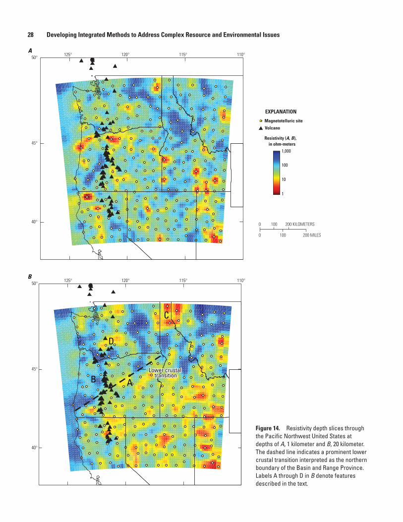
28 Developing Integrated Methods to Address Complex Resource and Environmental Issues
Figure 14. Resistivity depth slices through the Pacific Northwest United States at depths of A, 1 kilometer and B, 20 kilometer. The dashed line indicates a prominent lower crustal transition interpreted as the northern boundary of the Basin and Range Province. Labels A through D in B denote features described in the text.
D
C
B A
125° 120° 115° 110°
40°
45°
50°
125° 120° 115° 110°
40°
45°
50°
Resistivity (A, B), in ohm-meters
!( Magnetotelluric site
EXPLANATION
1
10
1,000
100
Volcano
Lower crustal transition
Lower crustal transition
B
A
0 200 KILOMETERS100
0 100 200 MILES

Method and Software Development 29
Improving Radar and Acoustic Imaging
By Karl J. Ellefsen
Issue and Scope
The U.S. Environmental Protection Agency delineates contaminants in the ground, and the U.S. Army Corp of Engineers delineates various types of heterogeneity in the ground. So, both agencies helped fund the development of a new method to process radar and acoustic data. Of course, this processing method also can be applied to radar and acoustic data collected for other purposes.
Although many methods have been developed to process radar and acoustic data, most require significant approxi-mations of the physics of wave propagation because such approximations simplify numerical simulation on a computer. Recently, the need for such approximations has diminished because inexpensive but powerful computers are readily available. For this project, the processing method requires few approximations. Thus, an image from this new method should better represent actual heterogeneity than an image from an older method.
Objectives
The objective of this work was to develop a method to estimate the properties of the ground using either radar traces or acoustic traces. The method was constrained to use only those computer resources that are typically available in a mod-ern personal computer. For example, the method could require multiple processor cores but not a cluster of computers.
Background
In the model used for the processing, locations are specified by a rectangular Cartesian coordinate system. The x–z plane of the model is divided into a grid of square cells. To each cell are assigned the model properties. Thus, model properties may vary in the x and z directions, but not in the y direction. The model properties are based on complex slow-ness because it is closely related to wave propagation. The model properties are the natural logarithm of the real part of the complex slowness log SR and the natural logarithm of the imaginary part of the complex slowness log SI.
The inversion is based on this objective function:
O(m) = (dc(m)−do)T Cd
–1 (dc(m)−do)*+(m−mp)
T Cm–1 (m−mp) (3)
where superscript T represents the transpose operation and the superscript * represents the complex conjugate operation. Vector m comprises log SR and log SI for every model cell. Vector mp is equivalent to vector m, except that it pertains to the reference model and is constant throughout the inversion.
Matrix Cm is the model covariance matrix. Vector do com-prises the observed data. These data are the recorded traces that are transformed from the time domain to the frequency domain. (Alternatively, these data can be just the amplitudes and traveltimes [phases] of the first arriving waves.) Vector dc(m) is similar to do, except that it comprises the calculated data for the current model. These data are computed from the numerical solution of the vector Helmholtz equation, which accounts for propagation in the y direction as well as the x and z directions, making the model two-and-one-half dimensional (2.5-D). Matrix Cd is the data covariance matrix.
The objective function O(m) is minimized using con-jugate direction and line search methods. The conjugate direction is used to change the model parameters causing the objective function to decrease. Because the objective function is nonlinear, this procedure must be applied repeatedly.
Results and Conclusions
The new method was evaluated, in part, by processing crosswell radar data that were collected in a laboratory tank. The tank was filled with dry, well-sorted sand to a depth of 1.61 meter (m). Embedded within the sand was an air-filled, plastic box for which the height and width were 0.178 and 0.121 m, respectively. Two vertical, air-filled wells, which were 0.78 m apart, penetrated almost all of the sand. These two wells were used to collect the radar data. The radar traces were recorded with a sample interval of 40 picoseconds, and the trace duration was 20 nanoseconds. The frequencies with high amplitudes ranged approximately from 0.4 to 1.5 Giga-hertz (GHz).
The crosswell radar data were used to estimate the model shown in figure 15. For this figure, the estimated log SR and log SI were converted to relative dielectric permittivity εr with the equation:
ε
µrR Is s
=−2 2
(4)
where μ is the magnetic permeability. The prominent, low-valued anomaly corresponds to the air-filled box. Within this anomaly, the smallest εr (1.58 [no units]) is larger than the corresponding εr for air (1 [no units]) because of the limited spatial resolution. Throughout the sand, there are numerous small anomalies, which are interpreted as changes in compac-tion, moisture content, and mineral composition. For example, in the lower right corner of figure 15, εr is relatively low compared to the rest of the sand, and this region is interpreted as poorly compacted sand. At depths less than 0.5 m, εr ranges from approximately 2.24 to 3.42 (no units), which is consis-tent with a laboratory-measured value of 2.71 (no units) at 0.95 GHz.
Some practical applications of this method include processing crosswell radar data and crosswell acoustic data. The processing could use either the complete traces or just the traveltimes and the amplitudes of the first arriving wave. Other practical applications include processing data collected with

30 Developing Integrated Methods to Address Complex Resource and Environmental Issues
an uncommon geometry (for example, surface to well) or an uncommon antenna orientation for radar data. The method has been used to estimate S-wave velocities using the traveltimes from an S-wave refraction survey (Ellefsen, 2009); of course, the method also could be used to estimate P-wave velocities using the traveltimes from a P-wave refraction survey.
Collaborators
U.S. Environmental Protection Agency, Office of Research and DevelopmentMineral Resource Program of the U.S. Geological SurveyToxics Substances Hydrology Program of the U.S. Geological SurveyU.S. Army Engineer Research & Development Center of the U.S. Army Corp of Engineers
Selected References
Burton, B.L., and Ellefsen, K.J., 2011, Phase inversion of refraction traveltimes: Environmental and Engineering Geo-physical Society, Proceedings of the Annual Symposium on the Application of Geophysics to Engineering and Environ-mental Problems, Charleston, South Carolina, p. 179–182 (CD-ROM).
Ellefsen, K.J., Croizé, Delphine, Mazzella, A.T., and McK-enna, J.R., 2009, Frequency-domain Green’s functions for radar waves in heterogeneous 2.5D media: Geophysics, v. 74, no. 3, p. J13–J22.
Ellefsen, K.J., 2009, A comparison of phase inversion and traveltime tomography for processing near-surface refraction traveltimes: Geophysics, v. 74, no. 6, p. WCB11–WCB24.
Ellefsen, K.J., Mazzella, A.T., Horton, R.J., and McKenna, J.R., 2010, Frequency domain, waveform inversion of laboratory crosswell radar data: Society of Exploration Geophysicists Expanded Abstracts, v. 29, p. 4019–4023, doi:10.1190/1.3513697.
Ellefsen, K.J., 2011, Computer programs for forward and inverse modeling of acoustic and electromagnetic data: U.S. Geological Survey Open-File Report 2011–1124, 11 p., http://pubs.usgs.gov/of/2011/1124/.
Ellefsen, K.J., Mazzella, A.T., Horton, R.J., and McKenna, J.R., 2011, Phase and amplitude inversion of cross-well radar data: Geophysics, v. 76, no. 3, p. G1–G12, doi:10.1190/1.3554412.
Peters, Bas, Moulton, C.W., Ellefsen, K.J., Horton, R.J., and McKenna, J.R., 2010, High-frequency, crosswell radar data collected in a laboratory tank: U.S. Geological Survey Digital Data Series 486, 19 p., plus digital data, http://pubs.usgs.gov/ds/486/.
Figure 15. Model estimated from the crosswell radar data. The model edges correspond to the boundary of the region probed by the radar waves. The black rectangle is the outline of the air-filled box.
Wel
l C
Wel
l B
0.0 1.0
1.5
1.0
0.5
0.5
0.0
Horizontal distance, in meters
Dept
h be
low
san
d-ai
r int
erfa
ce, i
n m
eter
s Relative dielectricpermittivity, unitless
1.74
3.25
1.91
2.07
2.24
2.41
2.58
2.75
2.92
3.08
3.42
1.57
EXPLANATION
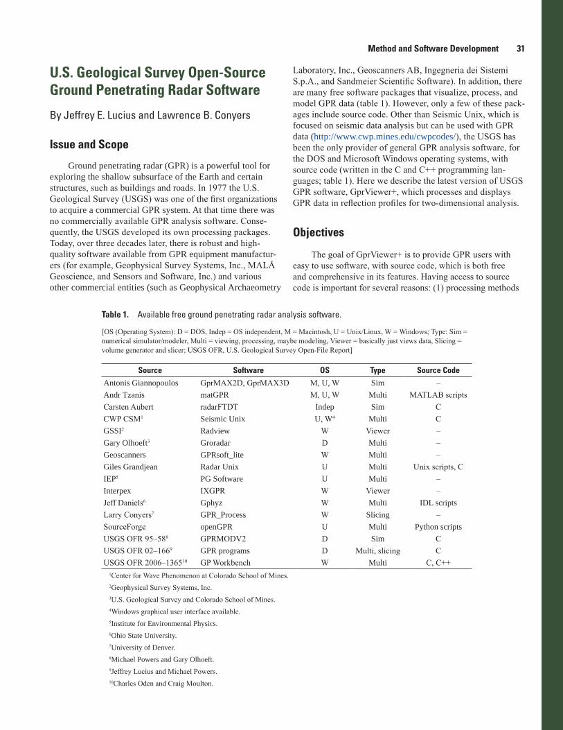
Method and Software Development 31
U.S. Geological Survey Open-Source Ground Penetrating Radar Software
By Jeffrey E. Lucius and Lawrence B. Conyers
Issue and Scope
Ground penetrating radar (GPR) is a powerful tool for exploring the shallow subsurface of the Earth and certain structures, such as buildings and roads. In 1977 the U.S. Geological Survey (USGS) was one of the first organizations to acquire a commercial GPR system. At that time there was no commercially available GPR analysis software. Conse-quently, the USGS developed its own processing packages. Today, over three decades later, there is robust and high-quality software available from GPR equipment manufactur-ers (for example, Geophysical Survey Systems, Inc., MALÅ Geoscience, and Sensors and Software, Inc.) and various other commercial entities (such as Geophysical Archaeometry
Laboratory, Inc., Geoscanners AB, Ingegneria dei Sistemi S.p.A., and Sandmeier Scientific Software). In addition, there are many free software packages that visualize, process, and model GPR data (table 1). However, only a few of these pack-ages include source code. Other than Seismic Unix, which is focused on seismic data analysis but can be used with GPR data (http://www.cwp.mines.edu/cwpcodes/), the USGS has been the only provider of general GPR analysis software, for the DOS and Microsoft Windows operating systems, with source code (written in the C and C++ programming lan-guages; table 1). Here we describe the latest version of USGS GPR software, GprViewer+, which processes and displays GPR data in reflection profiles for two-dimensional analysis.
Objectives
The goal of GprViewer+ is to provide GPR users with easy to use software, with source code, which is both free and comprehensive in its features. Having access to source code is important for several reasons: (1) processing methods
Table 1. Available free ground penetrating radar analysis software.
[OS (Operating System): D = DOS, Indep = OS independent, M = Macintosh, U = Unix/Linux, W = Windows; Type: Sim = numerical simulator/modeler, Multi = viewing, processing, maybe modeling, Viewer = basically just views data, Slicing = volume generator and slicer; USGS OFR, U.S. Geological Survey Open-File Report]
Source Software OS Type Source CodeAntonis Giannopoulos GprMAX2D, GprMAX3D M, U, W Sim –Andr Tzanis matGPR M, U, W Multi MATLAB scriptsCarsten Aubert radarFTDT Indep Sim CCWP CSM1 Seismic Unix U, W4 Multi CGSSI2 Radview W Viewer –Gary Olhoeft3 Groradar D Multi –Geoscanners GPRsoft_lite W Multi –Giles Grandjean Radar Unix U Multi Unix scripts, CIEP5 PG Software U Multi –Interpex IXGPR W Viewer –Jeff Daniels6 Gphyz W Multi IDL scriptsLarry Conyers7 GPR_Process W Slicing –SourceForge openGPR U Multi Python scriptsUSGS OFR 95–588 GPRMODV2 D Sim CUSGS OFR 02–1669 GPR programs D Multi, slicing CUSGS OFR 2006–136510 GP Workbench W Multi C, C++
1Center for Wave Phenomenon at Colorado School of Mines.2Geophysical Survey Systems, Inc.3U.S. Geological Survey and Colorado School of Mines.4Windows graphical user interface available.5Institute for Environmental Physics.6Ohio State University.7University of Denver.8Michael Powers and Gary Olhoeft.9Jeffrey Lucius and Michael Powers.10Charles Oden and Craig Moulton.

32 Developing Integrated Methods to Address Complex Resource and Environmental Issues
can be checked for accuracy; (2) object-oriented code can be reused; (3) using the original source code, the software can be modified and recompiled for execution; and (4) the algorithms and techniques can be instructional. This first version of the software has all the basic features needed by most users: read-ing and writing the standard data storage formats, conversion between storage formats, robust visualization (2-D only at this time), basic data processing operations, velocity analysis, publication-quality image exporting, and Windows printing. This software is designed for users who want to visualize and perform basic processing on multiple GPR data files in 2-D, without having to organize them into a project.
Background
In the 1980s the USGS (Gary Olhoeft and Jeffrey Lucius) developed GPR software written in HP Basic for HP 9845 and HP 9000 workstations. Around 1990 we started writing soft-ware in the C programming language for use on personal com-puters running DOS and early versions of Windows. Michael Powers wrote a 1-D, full-waveform, GPR modeling program, which was published with source code in 1995 (Powers and Olhoeft, 1995). In 2002, we published all our C-code GPR programs, which ran in DOS or in a command-prompt window in Windows (Lucius and Powers, 2002). As part of his devel-opment of GPR antennas at the USGS, Charles Oden wrapped some of our early C-code software and his new C++ code with a Windows graphical user interface (GUI) and published GP Workbench (Oden and Moulton, 2006).
From 2003 to 2005, the USGS and University of Denver (DU) developed GprViewr in the Java programming language. This first version of our GUI-based GPR analysis software could be run on any operating system that could utilize the Java Runtime Environment (JRE). Though not published, it has been used extensively at DU and by other users around the world. In 2010 we started development of the latest version of our software, now called GprViewer+. It is object-oriented software written in C# and will run in 32-bit or 64-bit Win-dows when .NET 4 (or later version) is installed. The first ver-sion of GprViewer+ should be ready for publication in 2015.
Results and Conclusions
GprViewer+ has the familiar Windows design and func-tionality, including standard menus and tool bars, status bar, and panels, which can be hidden or shown. It has “drag and drop” functionality for importing GPR data files. The most common GPR storage formats can be read, as well as the SEG-Y format. Files can be converted from one format to the other when saved. The Message Panel can display file headers, trace headers, the internal “GprInfo” object, which records all information avail-able about the GPR file and data, and messages.
Each GPR reflection profile appears in its own window. Switching between GPR windows can be accomplished in sev-eral different ways. There are a variety of window arrangements available including cascading, tile by columns, and tile by rows.
GPR data are initially displayed as depth or time on the vertical scale and distance or trace number on the horizontal scale. Nine preset color palettes are available. Zoom options include fixed multiplier, drawn-rectangle zoom, fit the window, fit the window width, fit the window height, or a 1-to-1 display (one sample for each screen pixel). If topographic information is supplied, the data can be topographically corrected for eleva-tion with optional vertical exaggeration enforced.
For the cursor position in the active GPR window, the status bar displays sample number, trace number, sample amplitude, sample time, and, if available, sample depth and trace distance. A wiggle-trace panel, showing the trace under the cursor, can be made visible or hidden within each GPR window.
At the present stage of development, GprViewer+ includes basic data processing, mostly available through the Processing Panel and tool bar: (1) trim data to user-selected first and last traces, (2) set time zero and nominal relative dielectric permit-tivity, (3) remove a background trace, (4) stack traces, (5) mix traces (using a sliding moving-average window), (6) apply amplitude gain with real-time image updates, and (7) use hyperbola fitting to determine radar wave velocity. The original data are stored internally and never manipulated. There are two copies of the data that are used for processing, one for tempo-rary display and one for saved changes. The original data can be restored at any time.
Future versions of GprViewer+ will include much more advanced data processing, drawing functions, numerical modeling, and 3-D voxel generation with slicing. Figures 16 and 17 show some of the features available at this time in GprViewer+.
Collaborators
GprViewer+ and earlier software were developed in coopera-tion with the University of Denver and funded by the USGS Integrated Methods Development Project, the USGS Toxic Substances Hydrology Program, and the U.S. Army Engineer Research & Development Center.
References Cited
Lucius, J.E., and Powers, M.H., 2002, GPR data processing computer software for the PC: U.S. Geological Survey Open-File Report 02–166, 101 p., also available at http://pubs.usgs.gov/of/2002/ofr-02-0166/.
Oden, C.P., and Moulton, C.W., 2006, GP Workbench man-ual—Technical manual, user’s guide, and software guide: U.S. Geological Survey Open-File Report 2006–1365, 81 p., also available at http://pubs.usgs.gov/of/2006/1365/.
Powers, M.H., and Olhoeft, G.R., 1995, GPRMODV2—One-dimensional full waveform forward modeling of dispersive ground penetrating radar data, version 2.0: U.S. Geological Survey Open-File Report 95–58, 41 p., also available at http://pubs.usgs.gov/of/1995/0058/report.pdf.

Method and Software Development 33
Figure 16. Example GprViewer+ screens. A, Main window with all panels and bars displayed. The same data file is shown in each window. The window on the left is how the file is initially displayed when opened, with the (optional) wiggle trace panel visible. The two windows on the right have been formatted using the Format Image dialog, and a background trace has been removed from the data. B, Examples of the Format Image dialog.
A
B

34
Developing Integrated Methods to Address Com
plex Resource and Environmental Issues
Figure 17. Example use of hyperbola fitting (to rebar reflections) for velocity analysis of concrete.

Method and Software Development 35
Potential-Field Software
By Jeffrey D. Phillips
Issue and Scope
For more than 60 years, the U.S. Geological Survey (USGS) has been developing software to process and display potential-field (gravity and magnetic) and other geophysical data. This software includes basic tools for editing, project-ing, and gridding scattered and flight-line data; tools for spatial and Fourier filtering of gridded and profile data; rudimentary tools for display of the data; and tools for the interpretation of the data using forward modeling, source parameter estimation, and inversion. In 1971, standard USGS data formats were adopted for grids and point data. This allowed computer programs written by different authors to work together as a coherent package, which became a research tool for prototyping new algorithms and extending the potential-field method.
At first programs were developed on IBM mainframe computers, then on VAX and Unix-based minicomputers, and, starting in 1989, on personal computers running the DOS operating system (Godson and Mall, 1989; Cordell and others, 1992; Phillips and others, 1993; Grauch and others, 1993). The last update of the DOS-based software package (Phil-lips, 1997) contained 246 executable programs and 36 batch scripts. Today the 16-bit DOS operating system has been replaced by 32-bit and 64-bit Windows operating systems requiring the use of new compilers and new strategies for maintaining this valuable software resource and applying it to USGS needs in the 21st century.
Objectives
The primary goal of this effort is an update of the USGS potential-field software package capable of running on 32-bit and 64-bit Windows-based computers. To make this package useful, both for current data processing needs and for future development of the potential-field method by USGS geophysi-cists, it must be based on open-source compilers and graphics toolkits, and it must use the standard USGS data formats for grids and point data.
A secondary goal is to distribute USGS potential-field software to the geophysical community at large, both as a stand-alone package and as plug-in modules to popular commercial geophysical software packages such as Geosoft Oasis-montaj (Geosoft, 1998). Although not as polished as commercial software, free geophysical software is valuable to students, professors, and individual researchers. Open-source software is an important resource for validation of results and for stimulating development of new methods and capabilities.
Background
Until the late 1990s, in-house development of potential-field geophysical software was the only option available to the USGS. This software was used for the processing of geophysi-cal data and the production of geophysical maps for publica-tion. By 1998, commercial geophysical software packages were offering data handling and map production capabilities far superior to those of the USGS software. In that year, the USGS entered into a long-term contract with Geosoft for mul-tiple licenses of Oasis-montaj. As part of the contract, USGS binary data formats for grids and point-data files were perma-nently incorporated into Oasis-montaj.
Although Oasis-montaj currently addresses the routine data processing and map production needs of the USGS, it has two disadvantages over in-house software: (1) the processing algo-rithms are hidden as “black-boxes,” so they cannot be examined in detail and (2) the package is not suitable for the rapid devel-opment of new algorithms for data processing or interpretation. To partially address the “black box” issue, Phillips and others (2003) and Phillips (2007) released 52 USGS potential-field algorithms as plug-in modules for Oasis-montaj, complete with source code. These Geosoft eXecutables or GXs provide an alternative to the Geosoft algorithms for basic grid utilities, spa-tial and Fourier filtering of grids, and grid interpretation. They also extend the capabilities of Oasis-montaj to include matched filtering of grids and new source-location algorithms.
Although GXs provide a way of incorporating USGS algorithms into Oasis-montaj, they are only useful for mature algorithms that are fully debugged. To develop new USGS algorithms and to preserve the old DOS algorithms, a Win-dows version of the USGS development environment has been assembled replacing 16-bit Microsoft Fortran and C compilers with a combination of open-source, 32-bit compilers (g77, gfortran, and gcc) and the Tcl/Tk graphical user interface (Welch and others, 2003; von Hagen, 2006). Several subrou-tine libraries of Webring (1998) have been used directly or modified to provide a new uniform command-line interface and access to binary files. PDEPTH (fig. 18), a graphical mag-netic- and gravity-profile-analysis program, is one example of a USGS program updated using this new environment. Release of a complete package of USGS Windows-based soft-ware is planned for the near future.
Results and Conclusions
USGS contributions to potential-field geophysics are documented in publications and in software (Bankey and Anderson, 1995). Most of the publications are readily avail-able, but much of the software has become out-of-date as personal computers have evolved. Converting outdated USGS software to GX plug-in modules, or to stand-alone programs that will run on modern computers, is the best way to maintain this legacy code. The development environments used for this preservation effort also permit the future development of the potential-field method at the USGS.

36 Developing Integrated Methods to Address Complex Resource and Environmental Issues
Collaborators
Misac Nabighian and Yaoguo Li, Colorado School of MinesMark Pilkington, Geological Survey of CanadaRichard Hansen (deceased) and Mike Hall, Edcon-PRJJim Roy, Northwest Geophysical Associates, Inc.Gerry Connard, GeosoftDes Fitzgerald, Intrepid GeoscienceMike Webring and Bob Simpson, USGS emeritiV.J.S. (Tien) Grauch and Richard J. Blakely, USGS
Figure 18. PDEPTH (a graphical magnetic- and gravity-profile-analysis program) is one example of a U.S. Geological Survey potential-field software program incorporating a graphical user interface. The ground-based magnetic profile (orange symbols in upper “profile” window) was collected on a surface (orange symbols in lower “section” window) just above the ground surface (upper gray line in section window, largely obscured by the orange observation surface symbols). Other gray lines in the section window represent geologic horizons and a fault extracted from a three-dimensional model. Vertical gray lines represent features such as bends in the line and intersections with other lines. Also scaled to fit within the profile window are the reduced-to-pole magnetic profile (red line, largely obscured by the orange observed magnetic profile symbols ), pseudogravity profile (purple line), and upward-continued pseudogravity profile (green line). The continuation surface (green line just above the section window) is 200 feet above the observation surface. Magnetic source locations estimated from upward-continued profiles are shown as green symbols (“C” for contact solutions and “S” for sheet solutions) in the section window. Dips of some sources are assumed to be vertical or horizontal; dips of other sources are estimated. Mouse-driven control buttons are on the right-hand side.
References Cited
Bankey, Viki, and Anderson, W.L., 1995, A bibliography of some geophysical computer programs, databases, and maps from the U.S. Geological Survey, 1971–1994: U.S. Geologi-cal Survey Open-File Report 95–77, unpaginated.
Cordell, Lindrith, Phillips, J.D., and Godson, R.H., 1992, U.S. Geological Survey potential-field geophysical software ver-sion 2.0: U.S. Geological Survey Open-File Report 93–18, 18 p., 6 diskettes.

Method and Software Development 37
Geosoft, 1998, OASIS Montaj Data Processing and Analysis (DPA) System for earth science applications, version 4.2, user guide: Geosoft, 268 p.
Godson, R.H., and Mall, M.R., 1989, Potential-field geophysi-cal programs for IBM compatible microcomputers, version 1.0: U.S. Geological Survey Open-File Report 89–197, 23 p., 5 diskettes.
Grauch, V.J.S., Phillips, J.D., Hoover, D.B., Pitkin, J.A., Livo, K.E., and McCafferty, Anne, 1993, Materials provided at the workshop “Geophysical Map Interpretation on the PC,” convened April 21–22, 1993: U.S. Geological Survey Open-File Report 93–560, 150 p., 14 diskettes (includes potential-field software update 2.11).
Phillips, J.D., 1997, Potential-field geophysical software for the PC, version 2.2: U.S. Geological Survey Open-File Report 97–725, 34 p., http://pubs.usgs.gov/of/1997/ofr-97-0725/pfofr.htm.
Phillips, J.D., 2007, Geosoft eXecutables (GX’s) developed by the U.S. Geological Survey, version 2.0, with notes on GX development from Fortran code: U.S. Geological Survey Open-File Report 2007–1355, 111 p., http://pubs.usgs.gov/of/2007/1355/.
Phillips, J.D., Duval, J.S., and Ambrosiak, R.A., 1993, National geophysical data grids—Gamma-ray, gravity, magnetic, and topographic data for the conterminous United States: U.S. Geological Survey Digital Data Series DDS–9, 1 CD-ROM, includes potential-field software version 2.1.
Phillips, J.D., Duval, J.S., and Saltus, R.W., 2003, Geosoft eXecutables (GX’s) developed by the U.S. Geological Sur-vey, version 1.0, with a viewgraph tutorial on GX develop-ment: U.S. Geological Survey Open-File Report 03–010, 23 p., http://pubs.usgs.gov/of/2003/ofr-03-010/.
von Hagen, William, 2006, The definitive guide to GCC: New York, NY, Apress, 584 p.
Webring, M.W., 1998, ODDF—A file I/O subroutine package implementing NASA PDS data description and USGS map projections, version 1.6: U.S. Geological Survey Open-File Report 98–765, 132 p., http://pubs.usgs.gov/of/1998/0765/report.pdf.
Welch, B.B., Jones, Ken, and Hobbs, Jeffrey, 2003, Practical programming in Tcl and Tk: Upper Saddle River, NJ, Pren-tice Hall PTR, 960 p.
Improving Geophysical Model Assessment with Bayesian Markov Chain Monte Carlo Methods
By Burke J. Minsley
Issue and Scope
Geophysical models are inherently uncertain due to the underlying measurement physics, data errors, acquisition geometry, and method of interpretation. But information about model uncertainty is rarely provided to nongeophysicist end-users be they hydrologists, geologists, or policy makers. Instead, geophysical results are often presented as a single “best” model. Although this simple product is often what the end-user wants, it can lead to misleading or incorrect interpretations. For example, if a geophysical model is displayed to a depth of 150 meters (m), it may be interpreted to that depth—even if the actual depth to which the data are sensitive is much shallower. When geophysical models disagree with co-located borehole data, it is often assumed that the geophysics is wrong, when in fact both models may be consistent with the measured data but are different because of equivalence and resolution issues. For these and many other reasons, the development of robust model assessment tools that can better inform nongeophysicists is criti-cal to advancing the value of geophysical data.
The focus of this work is to convey the characteristics of geophysical models that are consistent with measured data, rather than focus on the properties of any single model. This approach was popularized within the geophysical commu-nity by Albert Tarantola, who wrote “Practitioners usually seek the ‘best solution’ implied by the data, but observations should only be used to falsify possible solutions, not to deduce any particular solution” (Tarantola, 2006). Here, a Bayesian Markov chain Monte Carlo (MCMC) algorithm was devel-oped to assess the information contained in frequency-domain electromagnetic (FDEM) data, which are commonly acquired from both airborne and ground-based platforms by the U.S. Geological Survey (USGS). Whereas FDEM data are the focus here, the algorithm is readily adaptable to other geophysical methods, which will be the focus of future efforts.
Objectives
The objective of this work was to adapt and extend exist-ing Bayesian MCMC methods developed originally for direct-current resistivity surveys (Malinverno, 2002) for application to FDEM data. Because the algorithm can be readily modified for use with other types of geophysical data, this project is the base upon which future MCMC development will be founded. Initial applications for this work include model assessment and uncertainty analysis for airborne electromagnetic data acquired in western Nebraska (presented in the Results and Conclusions

38 Developing Integrated Methods to Address Complex Resource and Environmental Issues
section) and Alaska, as well as ground-based FDEM data from the Powder River Basin in Wyoming.
In addition to its use as a model assessment tool, the MCMC algorithm has also been modified to investigate instru-ment calibration errors (Minsley and others, 2011a,b). By gaging systematic instrument errors, correction factors can be derived that yield more accurate data which, in turn, lead to more accurate interpretations. Understanding data errors, both random and systematic, is absolutely critical for producing reliable results that can be interpreted with confidence. Infor-mation about reliability and model uncertainty is extremely relevant for USGS products that are available for use by deci-sion makers and the public.
Background
Stochastic parameter estimation techniques, as opposed to traditional deterministic inversion methods, have been utilized for some time to quantify uncertainty in geophysical inverse problems (Sambridge and Mosegaard, 2002). Advances in computational resources have made random search methods increasingly tractable for a growing class of parameter estima-tion problems. The primary benefit to stochastic methods is their ability to assess many viable models, rather than to focus on a single “best” model. In addition, many of the drawbacks of deterministic methods (such as the necessary linearization of the inverse problem and risk of finding solutions that are local, rather than global, minima) can be avoided using a stochastic approach.
The work of Malinverno (2002) and Sambridge and others (2006) has been adapted to perform model assess-ment FDEM geophysical datasets using a trans-dimensional Bayesian MCMC algorithm, the details of which can be found in Minsley (2011). This is a one-dimensional algorithm that produces an ensemble of many (tens to hundreds of thousands) layered-earth models of electrical resistivity as a function of depth that are consistent with the measured data. The main features of the algorithm are summarized below:
• Parameterization: Unknown parameters include layer interface depths and resistivity values within each layer. A unique feature of this algorithm is the fact that it is trans-dimensional, which means that the number of unknowns (that is, the number of layers) is one of the unknowns. That is, the number of layers is allowed to vary and the data, rather than a priori assumptions, are used to estimate the appropriate number of layers. This trans-dimensional aspect of the algorithm provides a substantial benefit in that solutions are not biased by a predetermined choice about the correct number of lay-ers. In addition, models with fewer layers are implicitly favored, which provides a natural measure of simplic-ity in the parameter assessment problem. In addition to the number of layers, interface depths, and resistivity values, the user can choose to estimate several optional parameters, including the level of random noise in the data, systematic instrument errors, and errors in the reported elevation of the FDEM system.
• Bayesian approach: According to Bayes theorem, each model is assigned a probability based on its fit to the data and how well it agrees with a priori assump-tions. In this work, the only prior information is that resistivity values should not oscillate wildly, which is based on the assumption that geologic properties do not vary significantly over short distances. This prior information is incorporated through a normal distribu-tion that penalizes models with thin layers that have large resistivity contrasts. The data fit is also described by a normal distribution that measures the differ-ence between observed and predicted data for a given model. The product of these two distributions is used to calculate the posterior probability for each sampled model. Although normal distributions are used here, it is straightforward to use any other probability density function that is appropriate.
• MCMC sampling: MCMC sampling is an effective tool for solving Bayesian problems where the posterior distribution cannot be evaluated analytically. MCMC sampling rules provide a guideline for proposing and accepting or rejecting models that, after a short “burn-in” period, are samples of the target posterior distribution. Each proposed model in the Markov chain depends only on the previous model in the chain. Making proposals that efficiently explore the space of plausible models is extremely important and is dis-cussed in detail by Minsley (2011). The algorithm runs for a prespecified number of samples are drawn or until some convergence criterion is met.
• Computational details: The FDEM trans-dimensional Bayesian MCMC algorithm is coded in Matlab. The computational bottleneck is in calculating the forward response to each proposed model; therefore, an efficient FDEM forward solver was written for Matlab, which utilizes multithreaded CPUs. The time for a single MCMC step is approximately 20 milliseconds (though it depends on the number of layers in the proposed model); therefore, a typical model assessment that sam-ples 100,000 models takes approximately 30 minutes.
Results and Conclusions
Compared with deterministic inversion algorithms, the MCMC method is significantly more computationally expen-sive but also contains much more information that can be used for model assessment and uncertainty analysis. For this reason, we utilize both methods together—the fast deterministic inver-sion algorithm is first run to provide an estimate of parameter values over an entire survey. Next, the MCMC algorithm is run at a few characteristic locations within the survey where information about uncertainty is needed.
An example of this approach from an airborne FDEM survey in western Nebraska (Smith and others, 2010) is pre-sented here. The primary goal of this survey was to map the
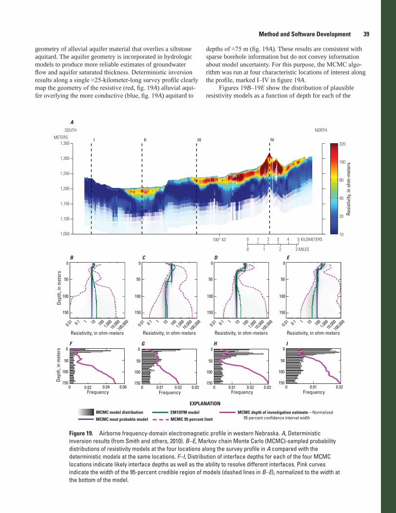
Method and Software Development 39
geometry of alluvial aquifer material that overlies a siltstone aquitard. The aquifer geometry is incorporated in hydrologic models to produce more reliable estimates of groundwater flow and aquifer saturated thickness. Deterministic inversion results along a single ≈25-kilometer-long survey profile clearly map the geometry of the resistive (red, fig. 19A) alluvial aqui-fer overlying the more conductive (blue, fig. 19A) aquitard to
depths of ≈75 m (fig. 19A). These results are consistent with sparse borehole information but do not convey information about model uncertainty. For this purpose, the MCMC algo-rithm was run at four characteristic locations of interest along the profile, marked I–IV in figure 19A.
Figures 19B–19E show the distribution of plausible resistivity models as a function of depth for each of the
MCMC depth of investigation estimate—Normalized 95 percent confidence interval width
MCMC model distribution EM1DFM modelMCMC 95 percent limit
B D
GF
EC
H I
I IVIIIIIMETERS
1,050
1,100
1,150
1,200
1,250
1,300
1,350
10
20
40
80
160
320
100° 43’
3
0 4321 5
0 21
KILOMETERS
MILES
NORTHSOUTH
A
Resi
stiv
ity, i
n oh
m-m
eter
s
0
50
100
150
Dept
h, in
met
ers
0
50
100
150
0
50
100
150
0
50
100
150
0.01 0.1
10,00
01,0
00100101
100,0
00
0
50
100
1500 0.01 0.02 0.03
0
50
100
1500 0.02 0.04 0.06
0
50
100
1500 0.01 0.02 0.03
0
50
100
1500 0.01 0.02
0.01 0.1
10,00
01,0
00100101
100,0
00 0.01 0.1
10,00
01,0
00100101
100,0
00 0.01 0.1
10,00
01,0
00100101
100,0
00
Resistivity, in ohm-meters Resistivity, in ohm-meters Resistivity, in ohm-meters Resistivity, in ohm-meters
Dept
h, in
met
ers
Frequency Frequency Frequency Frequency
EXPLANATION
MCMC most probable model
Figure 19. Airborne frequency-domain electromagnetic profile in western Nebraska. A, Deterministic inversion results (from Smith and others, 2010). B–E, Markov chain Monte Carlo (MCMC)-sampled probability distributions of resistivity models at the four locations along the survey profile in A compared with the deterministic models at the same locations. F–I, Distribution of interface depths for each of the four MCMC locations indicate likely interface depths as well as the ability to resolve different interfaces. Pink curves indicate the width of the 95-percent credible region of models (dashed lines in B–E), normalized to the width at the bottom of the model.

40 Developing Integrated Methods to Address Complex Resource and Environmental Issues
150
100
50
0
Resistivity, in ohm-meters0 100 200
−150
−100
−50
0
Formation factor
MCMC model distribution
MCMC most probable model
EM1DFM model
MCMC 95 percent limit
Short normal resistivity log
Long normal resistivity log
Gravel/gravelly soils
Sand/sandy soils
Silts and claysFormation factor
Dept
h, in
met
ers
10,0001,000100101 100,000
EXPLANATION
Figure 20. Markov chain Monte Carlo (MCMC)-sampled probability distribution from figure 19E compared with deterministic inversion result (green curve), borehole resistivity logs (yellow curves), and lithologic data (right panel). Although the “best-fit” inversion model appears to not agree with the borehole data, the MCMC analysis indicates that the frequency-domain electromagnetic data is also consistent with the borehole data, even though it is not the most probable model. EM1DFM is a software program (Farquharson and others [2003]).
four locations. These distributions are illustrated as shaded hit maps, where regions of the model with darker shading indicate a higher probability of a given resistivity value at the corresponding depth. Superimposed on each panel is the deterministic inversion result at that location (green curve) as well as the bounds that contain 95 percent of the MCMC sampled models (dashed magenta curves). These images con-vey information about the plausible range of resistivity values at depth and indicate the variable uncertainty associated with different sounding locations. Figures 19F–19I show histo-grams of the interface depths for all of the sampled MCMC models. In these panels, the peaks in the histogram indicate likely interface depths, and the width of the peak conveys details about how well resolved the interface is. For example, the base of the resistive aquifer at location II is much less well-defined than at location III due to the fact that it is much
deeper. The magenta curves in figures 19F–19I show the width of the 95-percent credible region bounds from figures 19B–19E and provide a quantitative metric for the depth of investigation, where there is a rapid increase in uncertainty beneath ≈50-m depth.
The resistivity distribution from figure 19E is reproduced in figure 20 along with downhole resistivity logs (yellow curves) and lithology information (right panel) from a bore-hole at the same location as the FDEM data. This location offers an example where the deterministic inversion result (green curve) appears to be inconsistent with the downhole data because it does not capture the increase in resistivity from ≈40–75 m depth. However, the MCMC results show that elevated resistivity values in this depth range are in fact consistent with the measured data. This illustrates the danger in interpreting the results of a single “best-fit” model.

Method and Software Development 41
Robust methods for quantifying the uncertainty associ-ated with geophysical models provide critical information for the end-users of geophysical datasets. The Bayesian MCMC approach implemented here has broad applicability for datas-ets acquired by the USGS, and will also be adapted for other types of data.
Selected References
Farquharson, C.G., Oldenburg, D.W.,and Routh, P.S., 2003, Simultaneous 1D inversion of loop–loop electromagnetic data for magnetic susceptibility and electrical conductivity: Geophysics, 68(6), 1857–1869, doi:10.1190/1.1635038.
Malinverno, Alberto, 2002, Parsimonious Bayesian Markov chain Monte Carlo inversion in a nonlinear geophysical problem: Geophysical Journal International, v. 151, no. 3, p. 675–688.
Minsley, B.J., 2011, A trans-dimensional Bayesian Markov chain Monte Carlo algorithm for model assessment using frequency-domain electromagnetic data: Geophysical Jour-nal International, v. 187, no. 1, p. 21.
Minsley, B.J., Hodges, Greg, Smith, B.D., and Abraham, J.D., 2011a, Multi-elevation calibration of frequency domain electromagnetic data: 17th European Meeting of Environ-mental and Engineering Geophysics of the EAGE, Leices-ter, England [invited paper].
Minsley, B.J., Hodges, Greg, Smith, B.D., and Abraham, J.D., 2011b, Multi-elevation calibration of frequency domain electromagnetic data: 24th Symposium on the Application of Geophysics to Engineering and Environmental Problems, Charleston, South Carolina.
Minsley, B.J., 2010, Improved geophysical model assess-ment using Bayesian Markov chain Monte Carlo Sampling [abs.]: American Geophysical Union 2010 Fall Meeting, San Francisco, Calif., December 13–17, 2010, Abstract NS13A-1163.
Minsley, Burke, 2010, Electrical resistivity parameter estima-tion and model appraisal using Bayesian inference, in S.R. Brady (ed.), Proceedings of the Third USGS Modeling Conference, June 7–11, 2010, Broomfield, Colorado—Understanding and Predicting for a Changing World: U.S. Geological Survey Scientific Investigations Report 2011–5147, p. 49.
Minsley, B., 2009, Assessing electrical resistivity model uncer-tainty using Bayesian inference [abs.]: EOS Transactions, American Geophysical Union, v. 90, no. 22, Joint Assembly Supplement, Toronto, Canada, Abstract NS13A-03.
Sambridge, Malcolm, and Mosegaard, Klaus, 2002, Monte Carlo methods in geophysical inverse problems: Reviews of Geophysics, v. 40, no. 3, p. 3–1.
Sambridge, Malcolm, Gallagher, Kerry, Jackson, Andrew, and Rickwood, Peter, 2006, Trans-dimensional inverse prob-lems, model comparison and the evidence: Geophysical Journal International, v. 167, no. 2, p. 528–542.
Smith, B.D., Abraham, J.D., Cannia, J.C., Minsley, Burke, Deszcz-Pan, Maria, and Ball, Lyndsay, 2010, Helicopter electromagnetic and magnetic geophysical survey data, por-tions of the North Platte and South Platte Natural Resources Districts, Western Nebraska, May 2009: U.S. Geological Survey Open-File Report 2010–1259, 33 p. http://pubs.usgs.gov/of/2010/1259/
Tarantola, Albert, 2006, Popper, Bayes and the inverse prob-lem: Nature Physics, v. 2, no. 8, p. 492–494.

Instrument Development
Development and Implementation of Passive Electrical Monitoring Arrays
By Burke J. Minsley and Paul A. Bedrosian
Issue and Scope
Passive electrical and electromagnetic measurements are widely used for the geophysical characterization of subsurface properties and processes (Bedrosian, 2007; Bedrosian and others, 2007; Linde and others, 2011). Monitoring applica-tions, however, require additional consideration as measuring systems must be deployed for long periods of time (weeks to months) and in harsh environments. Passive electrical
monitoring arrays comprise two main components: measuring electrodes that are placed in direct contact with the Earth and the necessary cabling and data-logging equipment that is con-nected to the electrodes. Both components of the system must be robust to diverse environmental conditions while providing reliable and stable measurements.
We summarize the development of a multichannel passive monitoring array that was deployed for 1 month at Kilauea Volcano, Hawaii, and later for 1.5 months underwater in the Great Salt Lake, Utah. In the Kilauea project, the system was utilized to monitor hydrothermal and magmatic processes at the volcano summit, whereas the Great Salt Lake study investigated submarine groundwater discharge. Both projects presented challenging environmental conditions that required the design of a multichannel monitoring system, which is not available commercially.
In addition, we have constructed a laboratory tank for monitoring and comparing the long-term sta-bility of different electrode designs. This controlled setting provides a platform for investigating the stability and noise characteristics of various types of electrodes and is used to select and match electrodes prior to taking them into the field. From a practical perspective, the tank is also ideal for maintaining electrodes, which tend to degrade if allowed to dry.
Objectives
Our primary objective was to design a versa-tile passive electrical monitoring array that could be deployed in harsh environmental conditions for a variety of monitoring applications and over a range of spatial scales and for durations of months or longer. Because of the requirements of the Great Salt Lake project, the system was designed not only to be weatherproof, but also to be capable of underwater installation. Other system requirements included inte-grated data storage to minimize manual data retrieval, ability to operate remotely with a solar-charged battery power supply, and need for a modular cable design to allow for flexibility in electrode geometry
BA
C D
EE
DC
BA
Figure 21. Electrical monitoring array. A, Multiconductor electrode cables, each with eight waterproof electrode takeouts at 20-meter intervals. B, Adapters for connecting bare-wire electrodes to the waterproof takeouts. C, Lead-lead chloride electrodes encased in bentonite and porous cloth bags to reduce contact resistance with the earth. D, Weatherproof box housing the data-logging system. Solar panel (not visible) is affixed to the box lid. E, Electrode test tank with datalogger. (USGS photographs)
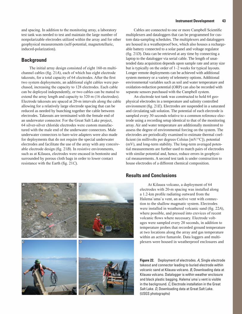
Instrument Development 43
and spacing. In addition to the monitoring array, a laboratory test tank was needed to test and maintain the large number of nonpolarizable electrodes utilized within the array and for other geophysical measurements (self-potential, magnetotelluric, induced-polarization).
BackgroundThe initial array design consisted of eight 160-m multi-
channel cables (fig. 21A), each of which has eight electrode takeouts, for a total capacity of 64 electrodes. After the first two system deployments, an additional eight cables were pur-chased, increasing the capacity to 128 electrodes. Each cable can be deployed independently, or two cables can be mated to extend the array length and capacity to 320 m (16 electrodes). Electrode takeouts are spaced at 20-m intervals along the cable allowing for a relatively large electrode spacing that can be reduced as needed by bunching together the cable between electrodes. Takeouts are terminated with the female end of an underwater connector. For the Great Salt Lake project, 64 silver-silver chloride electrodes were custom manufac-tured with the male end of the underwater connectors. Male underwater connectors to bare-wire adapters were also made for deployments that do not require the special underwater electrodes and facilitate the use of the array with any conceiv-able electrode design (fig. 21B). In resistive environments, such as at Kilauea, electrodes were encased in bentonite and surrounded by porous cloth bags in order to lower contact resistance with the Earth (fig. 21C).
Cables are connected to one or more Campbell Scientific multiplexers and dataloggers that can be programmed for cus-tom data-sampling schedules. The multiplexers and dataloggers are housed in a weatherproof box, which also houses a recharge-able battery connected to a solar panel and voltage regulator (fig. 21D). Data can be retrieved at any time by connecting a laptop to the datalogger via serial cable. The length of unat-tended data acquisition depends upon sample rate and array size but is typically on the order of 1–2 weeks for typical layouts. Longer remote deployments can be achieved with additional system memory or a variety of telemetry options. Additional environmental variables such as soil and water temperature and oxidation-reduction potential (ORP) can also be recorded with separate sensors purchased with the Campbell system.
An electrode test tank was constructed to hold 64 geo-physical electrodes in a temperature and salinity controlled environment (fig. 21E). Electrodes are suspended in a saturated and circulating salt solution. The potential of each electrode is sampled every 30 seconds relative to a common reference elec-trode using a recording setup identical to that of the monitoring array. Air and water temperature are additionally monitored to assess the degree of environmental forcing on the system. The electrodes are periodically examined to estimate thermal coef-ficient (in millivolts per degrees Celsius [mV/°C]), potential (mV), and long-term stability. The long-term averaged poten-tial measurements are further used to match pairs of electrodes with similar potential and, hence, reduce errors in geophysi-cal measurements. A second test tank is under construction to house electrodes of a different chemical composition.
Results and Conclusions
At Kilauea volcano, a deployment of 64 electrodes with 20-m spacing was installed along a 1.2-km profile radiating outward from the Halema`uma`u vent, an active vent with connec-tion to the shallow magmatic system. Electrodes were installed in weathered volcanic sand (fig. 22A), where possible, and pressed into crevices of recent volcanic flows where necessary. Electrode volt-ages were sampled every 20 seconds, in addition to temperature probes that recorded ground temperature at two locations along the array and gas temperature within an active fumarole. Data loggers and multi-plexers were housed in weatherproof enclosures and
Figure 22. Deployment of electrodes. A, Single electrode takeout and connector leading to buried electrode within volcanic sand at Kilauea volcano. B, Downloading data at Kilauea volcano. Datalogger is within weather enclosure and black plastic bagging. Halema`uma`u vent is visible in the background. C, Electrode installation in the Great Salt Lake. D, Downloading data at Great Salt Lake. (USGS photographs)
A B
C D
A B
C D

44 Developing Integrated Methods to Address Complex Resource and Environmental Issues
further wrapped in plastic bags to limit exposure to corrosive volcanic gases (fig. 22B). Batteries were changed and data recovered approximately every 10 days. The data are being analyzed in relation to volcanogenic processes, including pronounced deflation/inflation cycles of the summit area and magma drain/fill cycles within the Halema`uma`u vent (Bed-rosian and Kauahikaua, 2010).
In the Great Salt Lake, 64 electrodes were installed in loose sand beneath 20–40 cm of water (fig. 22C). The data recording equipment were housed in a Pelican case mounted on a platform built over the water (fig. 22D) and powered by a small solar panel. Electrodes were deployed along shore-parallel profiles extending 160 m in both directions from the datalogger, with 5–10 m electrode spacing. All 64 electrodes, plus one measure-ment of temperature and ORP in the water near the datalogger, were sampled every two minutes from June 17–August 4, 2010, resulting in nearly two million data points. Analysis of these data, combined with fiber optic distributed temperature measure-ments collected along a longer, subparallel profile, are ongoing.
Collaborators
Utah Water Science CenterUSGS Office of Groundwater, Branch of Geophysics Hawaiian Volcano ObservatoryUSGS Geology Venture Capital Fund
Selected References
Bedrosian, P.A., 2007, MT+, integrating magnetotellurics to determine Earth structure, composition, and processes: Sur-veys in Geophysics, doi:10.1007/s10712-007-9019-6.
Bedrosian, P.A., and Kauahikaua, James, 2010, Monitoring volcanic processes at Kilauea volcano with electrical and electromagnetic methods: Proceedings, 20th Workshop on Electromagnetic Induction in the Earth, Cairo, Egypt, 2010, 4 p.
Bedrosian, P.A., Unsworth, M.J., and Johnston, M.J.S., 2007, Hydrothermal circulation at Mount St. Helens determined by self-potential measurements: Journal of Volcanology and Geothermal Research, v. 160, no. 1–2, p. 137–146.
Linde, Niklas., Doetsch, Joseph, Jougnot, Damien, Genoni, O., Dürst, Yolanda, Minsley, B.J., Vogt, Tobais, Pasquale, N., and Luster, Jörg, 2011, Self-potential investigations of a gravel bar in a restored river corridor: Hydrology and Earth System Sciences, v. 15, no. 3, p. 729–742.
Development of a Waterborne Electromagnetic Survey System
By David V. Smith, Maria Deszcz-Pan, Daniel S. Scheirer, and Charles D. Blome
Issue and Scope
Airborne geophysical methods provide a cost-effective means of rapidly mapping electrical and magnetic properties over large areas of the Earth. Because these physical proper-ties are often diagnostic of rock types, such surveys can be a valuable tool for geologic mapping. Unless equipped with pontoons, commercial helicopter surveys undertaken in the United States are restricted from flying over open water by Federal Aviation Administration rules. In many places, com-plex geological structural features, such as faults, are under cover of water, inaccessible to field geologists.
Objectives
In areas of complex geology, it is often desirable to map structures that are under water to resolve, for example, fault traces, which are otherwise inferred. The objective of this work is to supplement airborne electromagnetic (EM) data with comparable data acquired on a freshwater lake using an EM bird mounted on a raft that is towed by a motorboat.
Background
The Lake of the Arbuckles in Chickasaw National Recreation Area was selected for waterborne electromagnetic (WEM) testing and evaluation because data from the lake would dovetail with data from a helicopter EM (HEM) survey flown in 2007 over an area bordering the lake to the east (Smith and others, 2011). An HEM bird originally developed for measuring sea ice thickness was mounted on a pontoon raft for operation on water. The EM bird was suspended inside a rectangular housing for ease of handling and protection from water. The raft also carried a magnetometer and a Q-coil for automatic calibration during the survey. The raft was towed by a motorboat, which carried the data acquisition systems for the EM bird and sonar bathymetry (fig. 23). In addition to EM data, accurate water depths were continuously measured along survey lines using a multibeam echo-sounder. Water-quality soundings were obtained at multiple locations to determine electrical conductivities of the water column, which will be used in subsequent data processing.
A theoretical model evaluated the sensitivity of the system to the geoelectrical parameters encountered in the lake environment. The model consisted of a 29 ohm-meter (Ω-m) water layer of varying thickness over a 20 Ω-m basement. Basement resistivity was estimated from the adjacent HEM survey measurements. The model showed that the expected

Instrument Development 45
system response significantly diminished for water depth greater than 5–10 m. Field data confirmed this result, showing flat responses over water deeper than about 7–10 m.
Results and Conclusions
The resolution of basement resistivity below the water layer depends on water depth, basement resistivity, and system parameters. Modeling showed that for a realistic system assuming 5 percent noise, detection of the 20 Ω-m basement is not pos-sible below 10-m water depth. Detection depth would increase for a more conductive basement (up to about 15 m for 10 Ω-m basement), a less conductive water column, or lower system noise. Lower HEM frequencies penetrate deeper than the higher frequencies and have lower signal levels. The lowest frequency collected with the WEM system was 15 kHz (kilohertz), and data analysis showed it was less affected by the problems with signal saturation than higher frequencies. The grids of appar-ent resistivity, at 15 kHz collected on the lake, suggest a general trend of higher resistivity in the northern arm of the lake, and lower resistivity along the northern shore of the eastern arm of the lake (fig. 24, bottom panel). These trends are consistent with the apparent resistivity grid based on 25 kHz HEM data (fig. 24, grid below flight lines, shown in blue) collected previ-ously with a different system. The inverted resistivity sections from both systems are also consistent with each other. This can be observed by comparing the two panels in figure 25, where the upper panel shows the inverted section of waterborne data, and the lower panel shows the inverted section based on HEM data. The dashed vertical lines show the extent of the overlapping seg-ments. The location of the section is indicated in figure 24B as the short white-line segment. The WEM inverted resistivity values are consistent with in situ measured water resistivity of 29 Ω-m. The inverted section of HEM data (fig. 25, lower panel) also gives resistivity values in the range 22–30 Ω-m. An example of inverted waterborne data for a longer line is given in figure 24A. The black line on the section traces the measured water depth.
Because the depth of investigation with the WEM is lim-ited to about 15 m in fresh water, valid measurements of the underlying geology whose resistivity is above 20 Ω-m can be acquired only in nearshore shallow areas. With this in mind, WEM surveys need to be run with closely spaced parallel lines conforming to the shoreline. Although deep water, such as the central areas of the Lake of the Arbuckles, precludes adequate signal, data collected over deep water, though not indicative of underlying geology, are crucial to system calibration. Central areas of the lake were too deep for adequate signal with the existing WEM bird. A bird with an operating frequency lower than 15 kHz would penetrate greater water depths. Accu-rate bathymetry is important to limiting the uncertainties in resolving basement resistivity using layered-earth inversions. Knowledge of water resistivity is essential for the success of this method.
Collaborators
Chickasaw National Recreation Area, a unit of the National Park ServiceOklahoma Water Resources Board
Selected References
Deszcz-Pan, Maria, Smith, D.V., and Smith, B.D., 2011, Application of an airborne HEM system on a freshwater lake: Environmental and Engineering Geophysical Society (EEGS) Symposium on the Application of Geophysics to Engineering and Environmental Problems (SAGEEP) 2011 Annual Meeting, Charleston, S.C., April 10–14, poster.
Smith, B.D., Smith, D.V., Deszcz-Pan, Maria, Blome, C.D., and Hill, Patricia, 2011, Helicopter electromagnetic and magnetic geophysical survey data, Hunton anticline, south-central Oklahoma: U.S. Geological Survey Open-File Report 2011–1240, 15 p.
Figure 23. Waterborne electromagnetic system consisting of watercraft for towing and data acquisition (left) and the electromagnetic bird mounted on a pontoon raft (right). (USGS photograph)

46 Developing Integrated Methods to Address Complex Resource and Environmental Issues
Figure 24. Apparent resistivity data. A, Inverted waterborne data along the selected waterborne transect where measured water depth is traced by a thin black line. B, Map of apparent resistivity for both surveys at the lowest waterborne frequency of 15 kHz (kilohertz) (over the lake area) and the closest 25 kHz frequency for airborne data (over land). The lines of helicopter electromagnetic data are shown in blue, waterborne lines are shown in green, with the selected waterborne transect shown in heavy black. The short white-line segment shows the waterborne transect overlapping the airborne line depicted in figure 25.
682,000 683,000Easting, in meters
−2,000
−1,000
0
1,000
2,000
Dis
tanc
e fro
m s
ectio
n, in
met
ers
240
250
260
270
Elev
atio
n, in
met
ers
A
B
10,000
10
15
17
22
29
50
150
Resistivity, in ohm-meters
20
30
35
75
100
0.1
EXPLANATION
681,000 684,000
0 1,000 METERS
0 2,000 FEET
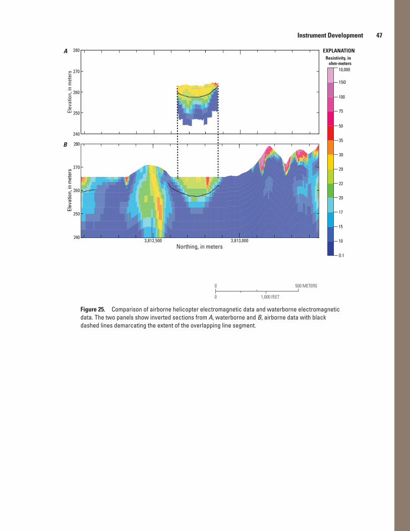
Instrument Development 47
280
240
250
260
270El
evat
ion,
in m
eter
s
3,813,0003,812,500Northing, in meters
240
280
250
260
270
Elev
atio
n, in
met
ers
Resistivity, in ohm-meters
10,000
0.1
35
50
75
100
150
22
29
30
10
15
17
20
EXPLANATIONA
B
0 500 METERS
0 1,000 FEET
Figure 25. Comparison of airborne helicopter electromagnetic data and waterborne electromagnetic data. The two panels show inverted sections from A, waterborne and B, airborne data with black dashed lines demarcating the extent of the overlapping line segment.

Minerals, Energy, and Climate
ore-forming solutions flow—of most hydrothermal mineral deposits. A fracture must be stressed, tectonically or hydrauli-cally, to near its point of failure in order for it to conduct the volumes of fluids necessary to form a hydrothermal mineral deposit. Therefore, by geophysically mapping fault and frac-ture systems in the subsurface using gravity and magnetic data and identifying the nature of these systems by anchoring the geophysical data to structural geologic data derived from field studies in the same area as well as developing models derived from experimental and analytical studies, we can reconstruct the paleo-orientation of tectonic stresses and the systematics of faulting, and then obtain a predictive model of the most likely locations within the mapped fault systems for focused fluid flow to have occurred and, in some circumstances, provide a framework for understanding mineral zoning in a district.
ResultsThe Boulder batholith, Montana, hosts one of the world’s
historically important copper resources in the Butte min-ing district and provides an opportunity to study the tectonic context of a batholith, the structural evolution of its com-ponent parts, and the relation of mineralization-controlling faults to this tectonic/structural story. Detailed geologic maps of the batholith allow its internal structural evolution to be interpreted, and the analysis of magnetic and gravity data allow the structural evolution of the batholith to be put into a tectonic context (see Berger and others, 2011). Figure 26 shows the topography on the basal surface of Butte Quartz Monzonite intrusion, the largest single pluton and core of the batholith. The solid white line shows the geophysical outer margin of the whole batholith; the inner dashed white line is the outer boundary of Butte Quartz Monzonite. Butte Quartz Monzonite has a generally hour-glass shape and flat bottom at 6–8 kilometer (km) depth. Two zones with calculated depths of 13–15 km are suggestive that Butte Quartz Monzonite was intruded through two separate zones at the base and forms two funnel-shaped masses that coalesced to give an appar-ent single intrusion in map view. This geometry is consistent with a model that Butte Quartz Monzonite was intruded into a structural pull-apart (for example, Schmidt and others, 1990) formed behind the advancing Montana Disturbed Belt thrust front. The axis of symmetry of this pull-apart is coincident with a zone of faulting trending northeast from Butte to the northeast margin of the batholith that has been interpreted (Schmidt and others, 1990) to be a deep-seated, Precambrian fault zone. The Butte mining district is localized within this axially symmetric fault zone and associated with the southern part of the inferred Butte Quartz Monzonite feeder zones.
The mineralized veins in the Butte district form overlap-ping sets of fanning or horsetailing faults (fig. 27) that step from northwest to southeast across the fault zone that makes up the axis of symmetry of the pull-apart structure within
Integrated Structural Geologic and Potential-Field Geophysical Studies to Understand the Spatial Localization of Magmatic-Hydrothermal Mineral Deposits
By Byron R. Berger, Thomas G. Hildenbrand, and J. Michael O’Neill
Issue and Scope
Most of the mineral deposits that crop out on Earth’s surface have been explored, and the greatest potential for undiscovered deposits is in favorable rocks buried beneath cover materials. Predicting the locations of undiscovered, bur-ied mineral deposits is a major source of uncertainty to geolo-gists engaged in mineral-resource assessments and minerals exploration. To reduce the uncertainty and accurately predict covered deposit locations, it is necessary to better understand the phenomena important in the localization of mineralizing systems and the mechanisms that facilitate the formation of ore bodies within mineralizing systems.
Objectives
To form an economic hydrothermal mineral deposit, it takes a large volume of hot fluid flowing at high rates that must be sustained for a significant length of time. This necessitates that connected fault and fracture permeability plays a dominating role in mineral deposit formation, and, consequently, there is a need to understand the permeabil-ity structure of mineral-deposit-forming environments and how they evolve in a dynamic setting. Our research has two primary objectives. Through the study of known mining districts and deposits, a first objective is to understand the permeability structure of connected fault and fracture systems at the mineral-district and ore-body scales. A second objective is to understand how the permeability structure changes in response to active seismicity and concurrent hydraulic stress. To achieve these objectives, we integrate structural geologic and magnetic and gravity geophysical data to construct models of known mineralized systems to use as analogs in the analysis of covered terrains.
BackgroundInterconnected networks of faults and fractures dominate
the permeability structure—the channelways along which

Minerals, Energy, and Climate 49
Figure 26. Calculated depths to the base of Butte Quartz Monzonite using a 3-D gravity inversion model. The model shows that Butte Quartz Monzonite forms an hour-glass shaped, flat slab that was likely derived principally from two feeder zones. The arrows indicate where the base of the batholith appears to pinch inward coincident with higher density batholithic rocks as indicated by magnetic data. The anomaly associated with the Deer Lodge Valley is a modeling edge effect. From Berger and others (2011).
−2.4
−1.2
0.0
1.2
2.4
3.6
4.8
6.0
7.2
8.4
9.6
10.8
12.0
13.2
14.4
Feeder?
Denser granodiorite
at depth?
Feeder?
Butte
Deer
Lodg
e V
alle
y
Depth, in kilometers
112°40' 112°00'
46°00'
46°40'
EXPLANATION
N
0 20 KILOMETERS10
0 10 20 MILES

50 Developing Integrated Methods to Address Complex Resource and Environmental Issues
which Butte Quartz Monzonite intruded. All of the faults are parallel to local, pre-existing joint trends in the Butte Quartz Monzonite and were likely guided by these joint weaknesses. The faults are interpreted to be sets of segmented, northeast-striking right-lateral “master” faults along which small splay or wing faults developed at the fault tips, again following ante-cedent fracture trends, on one or both sides of northeast fault segments and then propagated away from the tips to ultimately form the observed networks of northeast, east–west, and northwest striking faults. In figure 27, each interpreted fault set is color coded to aid differentiation. In figure 28, the faults are color coded to differentiate those veins that were silver-rich versus copper-rich. From figure 28 it can be inferred that the first two fanning fault sets to the northwest (purple and blue in fig. 27) formed a linked-fluid upflow compartment that was physically separate and chemically different from the sets to the southeast. Intermingling of the two fluids from the two upflow zones occurred only in the northwest part of the district where silver- and copper-rich veins are known to mutually crosscut the other.
Conclusions
Integrating structural geologic data interpretations and state-of-the-art interpretative techniques of potential-field geo-physical data provides insights as to how (1) pre-mineralization structures affect subsequent fault and fracture deformation events, (2) different processes couple to localize igneous intru-sions, and (3) ore-localizing fault and fracture permeability develops, and the mechanisms through which deformation can lead to focused fluid flow. Studies in the Butte mining district show how integrated studies in batholithic terranes can reduce uncertainties in mineral-resource assessments and reduce risk in exploration activities in analogous terranes. Reduced risk comes from a better understanding of why mineral deposits are localized where they are in batholithic terranes, which, in turn, reduces the area of search.
Acknowledgments
Byron (Barney) Berger passed away on December 10, 2013, after a long battle with cancer. During his 36 years at the U.S. Geological Survey, Barney became an internation-ally prominent economic geologist specializing in quantitative mineral resource assessments and ore genesis research. He authored or co-authored nearly 50 papers on the geology and geochemistry of ore deposits. He also served in a USGS lead-ership role as branch chief of the Exploration Geochemistry Branch and later of the Geochemistry Branch.
Related Project References
Berger, B.R., 2007, The 3D fault and vein architecture of strike-slip releasing and restraining bends–Evidence from volcanic-centre-related mineral deposits, in Cunningham, W.D., and Mann, P., eds., Tectonics of strike-slip restraining and releasing bends: Geological Society of London Special Publication 290, p. 447–471.
Berger, B.R., Anderson, R.E., Phillips, J.D., and Tingley, J.V., 2005, Plate-boundary transverse deformation zones and their structural roles in localizing mineralization in the Virginia City, Goldfield, and Silver Star mining districts, Nevada, in Rhoden, H.N., Steininger, R.C., and Vikre, P.G., eds., Geological Society of Nevada Symposium 2005—Window to the world: Geological Society of Nevada, Reno, p. 269–281.
Berger, B.R., Tingley, J.V., and Drew, L.J., 2003, Structural localization and origin of compartmentalized fluid flow, Comstock Lode, Virginia City, Nevada: Economic Geology, v. 98, p. 387–408.
Blakely, R.J., John, D.A., Box, S.E., Berger, B.R., Fleck, R.J., Ashley, R.P., Newport, G.R., and Heinemeyer, G.R., 2007, Crustal controls on magmatic-hydrothermal systems—A geophysical comparison of White River, Washington, with Goldfield, Nevada: Geosphere, v. 3, p. 91–107.
Hildenbrand, T.G., Berger, B.R., Jachens, R.C., and Lud-ington, S.D., 2000, Regional crustal structures and their relation to the distribution of ore deposits in Western United States based on magnetic and gravity data: Economic Geol-ogy, v. 95, p. 1583–1603.
Hildenbrand, T.G., Berger, Byron, Jachens, R.C., and Luding-ton, Stephen, 2001, Utility of magnetic and gravity data in evaluating regional controls on mineralization—Examples from the Western United States: Society of Economic Geologists Reviews in Economic Geology, v. 14, p. 75–109.
References Cited
Berger, B.R., Hildenbrand, T.G., and O’Neill, J.M., 2011, Control of Precambrian basement deformation zones on emplacement of the Laramide Boulder batholith and Butte mining district, Montana, United States: U.S. Geological Survey Scientific Investigations Report 2011–5016, 29 p.
Schmidt, C.J., Smedes, H.W., and O’Neill, J.M., 1990, Syn-compressional emplacement of the Boulder and Tobacco Root batholiths (Montana-USA) by pull-apart along old fault zones: Geological Journal, v. 25, p. 305–318.

Minerals, Energy, and Climate 51
Figure 27. Complex networks of linked, fanning, or horsetailing faults color coded to show how groups of faults may have grown as a set. The sets developed in a manner that eventually kinematically linked the northwesternmost northeast “master” (controlling) fault to the southeasternmost “master” fault. After Berger and others (2011).
Figure 28. Map of polymetallic quartz veins and faults in the Butte mining district. Those veins and associated faults that were predominantly mined for silver are color coded differently from those veins and faults predominantly mined for copper. From Berger and others (2011).
EXPLANATION
Arrows indicate sense of displacement on northeast-striking strike-slip faults.
N
MC
L2K
A
S
Lx
Continental deposit
Berkeleydeposit
CON
TIN
ENTA
LFA
ULT
0 500 METERS
0 2,000 FEET
L2
EXPLANATIONCopper-rich zone
Silver-rich zone
Northeast-striking veins and faults Fault, undivided
Mine shaft
Mine shaft name
General outline of porphyry-style deposit
East- to west–striking veins and faultsNorthwest-striking veins and faults
Northeast-striking veins and faultsNorthwest-striking veins and faults
Extensional stepover faults between the Berkeley and Continental porphyry-style deposits
MONTANA

52 Developing Integrated Methods to Address Complex Resource and Environmental Issues
Geophysical Support for Global Mineral Resource Assessments
By Jeffrey D. Phillips and Byron R. Berger
Issue and Scope
Mineral resource assessments conducted by the U.S. Geological Survey (USGS) of areas within foreign countries often must rely on interpretative products such as published geologic maps and cross sections that may not conform to our current understanding of global tectonics. Geophysical data, such as regional or global aeromagnetic compilations, offer a synoptic view of the upper crust and provide an unbiased framework for comparative understanding of the regional tectonics, identification of tectonic boundaries, and subdivi-sion of terranes into different domains based on geophysi-cal attributes. One of the early steps in any mineral resource assessment involves identifying the boundaries of geologically permissive areas or “tracts” where a specific mineral deposit type might occur. Geophysically determined tectonic bound-aries can help guide the establishment of tract boundaries where the basement geology is uncertain or is concealed under sedimentary, volcanic, or structural cover.
Objectives
The goal of this effort was to incorporate regional geo-physical data, primarily crustal magnetic anomaly data, into global mineral resource assessments. The magnetic anomaly data were used to supplement available geologic maps and aid in the interpretation of major tectonic features such as magmatic arcs of various ages, the occurrence of favorable geologic units such as intrusive rocks, and the boundaries of intrusive complexes that constitute permissive terranes for specific types of mineral deposits.
Background
Due to contractual agreements and copyright restrictions, high-quality aeromagnetic data are rarely available at an afford-able price for most foreign countries. Canada and Australia are two exceptions. Compiled aeromagnetic grids are avail-able for some countries such as Mexico and the former Soviet Union (U.S.S.R.). A global magnetic anomaly grid at a 2-arc minute (3.7 kilometer [km] or better) resolution compiled from aeromagnetic, shipborne magnetic, and satellite magnetic data is available from the National Oceanographic and Atmospheric Administration (NOAA) (Maus and others, 2009).
During a recent USGS global assessment of porphyry copper resources, magnetic anomaly data from the global grid and from the former U.S.S.R. grid were used to support tec-tonic interpretations in several areas including Europe, eastern Europe, Mongolia, eastern Russia, Iran, the southern Urals,
and Central Asia. Here we illustrate the use of these geophysi-cal data through an example from the western Central Asia assessment (Berger and others, 2014).
Results and Conclusions
An aeromagnetic dataset for the former U.S.S.R is available in digital form on CD-ROM from the NOAA National Geophysi-cal Data Center (NGDC, 1997). At the highest resolution, these data were sampled in a 2,500-meter grid in order to be useful for examining the longer wavelength components of the aeromag-netic field. These data were used to produce a grid of long-wave-length aeromagnetic anomalies for the Central Asia study area.
The aeromagnetic grid was reduced to the pole using proprietary software. Reduction-to-the pole (RTP) is a filtering process that removes the effect of geomagnetic latitude and repositions magnetic anomalies directly over their sources (Blakely, 1995). As a first step toward interpretation, the hori-zontal gradient magnitude of the RTP aeromagnetic grid was calculated, and the lines of maximum horizontal gradient were extracted. These lines define potential locations of vertical (steeply dipping) magnetic contacts within the crust (Cordell and Grauch, 1985; Blakely and Simpson, 1986; Grauch and Cordell, 1987). The lines were superimposed on the RTP aeromagnetic map to aid in geologic interpretation and the selection of tract boundaries (fig. 29).
These geophysical boundaries were used for defining tract boundaries in areas where no clear boundaries could be determined from the mapped geology (see heavy white and dashed black lines in fig. 29). The ability to draw these bound-aries in covered or poorly mapped areas reduced the overall level of uncertainty in the assessment.
Collaborators
Jane M. Hammarstrom and Michael L. Zientek, Project Chiefs, USGS Global Mineral Resource Assessment Project
References Cited
Berger, B.R., Mars, J.C., Denning, P.D., Phillips, J.D., Ham-marstrom, J.M., Zientek, M.L, Dicken, C.L., and Drew, L.J., with contributions from Alexeiev, Dmitriy, Seltmann, Reimar, and Herrington, R.J., 2014, Porphyry copper assess-ment of western Central Asia: U.S. Geological Survey Scien-tific Investigations Report 2010–5090–N, 219 p., 8 plates, and spatial data, http://dx.doi.org/10.3133/sir20105090N.
Blakely, R.J., 1995, Potential theory in gravity and magnetic applications: Cambridge, United Kingdom, Cambridge University Press, 441 p.
Blakely, R.J., and Simpson, R.W., 1986, Approximating edges of source bodies from magnetic or gravity anomalies: Geo-physics, v. 51, no. 7, p. 1494–1498.

Minerals, Energy, and Climate 53
Figure 29. Generalized tectonic map (after Chitalin, 1996) of the Spasski fold belt in Central Asia, plotted on top of a color shaded-relief, reduced-to-pole aeromagnetic map. Red colors indicate magnetic highs; blue colors indicate magnetic lows. Thin white lines give locations of the maximum horizontal gradients of the reduced-to-pole magnetic field; these may correspond to steeply dipping magnetic contacts representing crustal boundaries. The fold belt separates the Zharman-Sarysu (ZS) accreted terrane of Windley and others (2007) from the northern part of the Devonian magmatic arc (D) that overlaps the Zharman-Sarysu terrane on its east and west margins. Also shown is the Carboniferous Balkhash-Ili magmatic arc (BI). Faults, shown in light-gray lines, are from Seltmann and others (2009). The map area is north and northwest of Lake Balkhash, north-central Kazakhstan. The latitude, longitude, and location of the city of Karaganda were approximated using Google Earth.
Chitalin, A.F., 1996, Variscan structural evolution of central Kazakhstan, in Shatov, V., Seltmann, R. Kremenetsky, A., Lehmann, B., Popov, V., and Ermolov, P., eds., Granite-related ore deposits of central Kazakhstan and adjacent areas: St. Petersburg, GLAGOL Publishing House, p. 93–102.
Cordell, Lindrith, and Grauch, V.J.S., 1985, Mapping base-ment magnetization zones from aeromagnetic data in the San Juan Basin, New Mexico, in Hinze, W.J., ed., The util-ity of regional gravity and magnetic anomaly maps: Society of Exploration Geophysicists, p. 181–197.
Grauch, V.J.S., and Cordell, Lindrith, 1987, Limitations on determining density or magnetic boundaries from the hori-zontal gradient of gravity or pseudogravity data: Geophys-ics, v. 52, no. 1, p. 118–121.
Maus, S, Barckhausen, U., Berkenbosch, H., Bournas, N., Brozena, J., Childers, V., Dostaler, F., Fairhead, J.D., Finn, C., von Frese, R.R.B., Gaina, C., Golynsky, S., Kucks, R., Lühr, H., Milligan, P., Mogren, S., Müller, R.D., Olesen, O.,
Pilkington, M., Saltus, R., Schreckenberger, B., Thébault, E., and Caratori Tontini, F., 2009, EMAG2—A 2-arc min resolution Earth magnetic anomaly grid compiled from satellite, airborne, and marine magnetic measurements: Geochemistry, Geophysics, Geosystems, v. 10, Q08005, doi:10.1029/2009GC002471, 12 p.
National Geophysical Data Center (NGDC), 1997, Magnetic anomaly data of the former Soviet Union: National Oceano-graphic and Atmospheric Administration, National Geo-physical Data Center CD-ROM, unpaginated.
Seltmann, R., Shatov, V., and Yakubchuk, A., 2009, Min-eral deposits database and thematic maps of Central Asia, explanatory notes: London, Natural History Museum, Cen-ter for Russian and Central Asian Mineral Studies, 174 p.
Windley, B.F., Alexeiev, Dmitriy, Xiao, Wenjiao, Kröner, Alfred, and Badarch, Gombosuren, 2007, Tectonic models for accretion of the Central Asian orogenic belt: Journal of the Geological Society of London, v. 164, p. 31–47.
Karaganda50°
48°
73°71° 75° 77°
D
D
BI
ZS
ZS
EXPLANATION
Outer boundary of Carboniferous magmatic-arc rocks
Outer boundary of Devonian magmatic-arc rocks
High-angle faults, undifferentiated
Previously mapped faults (Seltmann and others, 2009)
Low
High
Magnetic field
Maximum horizontal gradient
0 100 KILOMETERS50
0 25 50 MILESMiddle Carboniferous thrust faults
Late Carboniferous to Permian thrust faults

54 Developing Integrated Methods to Address Complex Resource and Environmental Issues
U.S. Geological Survey Cooperative Research on Carbon Dioxide Sequestration Using Ultramafic and Carbonate Rocks
By Anne E. McCafferty, William H. Langer, and Bradley S. Van Gosen
Issue and Scope
Over geologic time, the natural weathering of carbonate and ultramafic rocks at and near the Earth’s surface captures and sequesters atmospheric carbon dioxide (CO2). Reducing CO2 in the atmosphere that is emitted from fossil-fuel-fired power plants will require a range of carbon management and sequestration options. Two emerging carbon storage methods that attempt to speed up the natural weathering processes are mineral CO2 sequestration (also known as mineral carbonation) and accelerated weathering of limestone (AWL). One respon-sibility of the U.S. Geological Survey (USGS) is to provide critical geologic information at a national scale to underpin the chemical and industrial research and development of mineral resources. In the case of ultramafic rocks, the USGS also provides information on how geophysical data can be used to extend and refine the geologic mapping of ultramafic rocks.
Objectives
One of the first tasks to address the viability of both these approaches is to estimate the available mineral resources. For this initial estimation, the USGS produced national-scale geologic maps that show calcium-rich lime-stone and magnesium-rich ultramafic rocks (fig. 30). These maps were produced in cooperation with researchers from the Earth Institute at Columbia University (http://www.energy.columbia.edu/), the University of California, Santa Cruz (http://ims.ucsc.edu/facres/index.html), and the Carn-egie Institution for Science (http://dge.stanford.edu/labs/caldeiralab). These national-scale maps detail the geographi-cal distribution and extent of rocks suitable for use in accel-erated weathering of limestone (fig. 30A) and mineral CO2 sequestration with ultramafic rocks (fig. 30B), respectively.
Background
Accelerated Weathering of LimestoneAccelerated weathering of limestone is proposed as a
low-tech method to capture and sequester CO2 that is expelled from fossil-fuel-fired power plants and other point-sources, such as cement manufacturing plants. AWL combines captured CO2 with water and calcium carbonate to produce water that is rich in bicarbonate ions. This slurry can be released in the
ocean with little or no apparent negative environmental impact (Caldeira and Rau, 2000). Rocks rich in calcium carbonate, particularly limestone, are ideally suited for this process. The large amounts of pulverized limestone (“fines”) produced dur-ing the processing of crushed limestone may be useful in this method of CO2 sequestration, providing finely ground calcium carbonate for use in the slurry mixture.
Mineral Carbonation Using Ultramafic Rocks
Mineral storage of CO2 occurs in nature through chemical reactions during the weathering of ultramafic rocks. When it rains, the rainwater mixes with CO2 in the atmosphere to form a weak carbonic acid. The carbonic acid reacts with mag-nesium-silicate minerals—which are abundant in ultramafic rocks—to form a solid magnesium-carbonate rock called magnesite (MgCO3). In this manner, CO2 gas is permanently “locked up” in the magnesite as a solid.
Rates of natural mineral carbon sequestration vary with geologic conditions but typically occur too slowly to make it an effective immediate means to sequester carbon dioxide from industrial sources. Hence, research organizations are exploring ways to chemically, thermally, or mechanically accelerate and enhance the natural process through an indus-trial process that is timely and economically viable (Matter and Kelemen, 2009; Zevenhoven, 2010). Advantages to this type of sequestration is that magnesite is a stable mineral at the Earth’s surface, it has no legacy issues (such as acid drain-age), and would require no monitoring after disposal, because magnesite remains environmentally benign over geologic time scales. Additionally, large amounts of waste rock generated from the past mining of asbestos in ultramafic rocks could be considered as source material for the mineral carbonation pro-cess. Asbestos minerals are very reactive and as such are some of the first minerals to dissolve in the mineral carbonation process, thereby providing a means to simultaneously mitigate both a climate and human health hazard.
Results and Conclusions
A feasibility study conducted by the USGS for carbon sequestration through an accelerated weathering of limestone operation requires access to an inexpensive source of lime-stone and to seawater; these parameters limit AWL facilities to within about 10 kilometers (km) of the coastline (fig. 30A). The majority of U.S. power-generating facilities in coastal areas are within economical transport distance of limestone resources (Langer and others, 2009). AWL presents opportunities for col-laborative efforts between the crushed stone industry, electrical utilities, cement manufactures, and research scientists.
The USGS, in cooperation with the Earth Institute at Columbia University, released a national-scale map of mag-nesium-rich ultramafic rocks for mineral CO2 sequestration in both report and digital map form (Krevor and others, 2009). The report identifies the largest known sources of ultramafic bedrocks

Minerals, Energy, and Climate 55
Figure 30. National-scale maps of A, carbonate rocks and B, magnesium-rich ultramafic rocks (in red) thought suitable for carbon dioxide sequestration in the conterminous United States. Circles on A show locations of power plants along coastal areas; colors indicate distance from power plants to carbonate rock. Modified from Krevor and others (2009). km, kilometers; Mg, magnesium.
in the continental United States (fig. 30B). In total, the map shows 16,263 km2 of ultramafic rocks, an area roughly equivalent to the State of Hawaii including all its islands. Scientists from Columbia University estimate this is enough material to seques-ter 500 years of carbon dioxide at 2009 levels of emissions.
In addition, the USGS extended the geologic mapping of the ultramafic rocks to include geophysical methods to map the volume, area, and depth of ultramafic rock masses (McCafferty
and others, 2009). Ultramafic rocks contain magnetic miner-als that make them ideal targets for aeromagnetic surveying. Mathematical enhancements can be applied to magnetic survey data to enhance anomalies that occur over ultramafic rocks (fig. 31). These enhancements allow for detailed examination of ultramafic rocks that may be completely or shallowly buried, which allows for a more robust assessment and characterization of rock material available for mineral carbonation.
A BBA
B
1 km2 to 10 km11 to 50 km51 to 100 km
101 to 200 km201 to 300 km301 to 400 km
Distance from powerplants to limestone
EXPLANATION
Limestone
Mg-rich ultramafic rock
EXPLANATION

56 Developing Integrated Methods to Address Complex Resource and Environmental Issues
Collaborators
Sam Krevor, Stanford University Global Climate & Energy Project, Stanford University, California Gregory Rau, Research Marine Scientist, Institute of Marine Sciences, University of California, Santa Cruz Ken Caldeira, Senior Scientist, Department of Global Ecology, Stanford University
For Additional Information
U.S. Geological Survey data and studies related to this topic can be found at http://crustal.usgs.gov/projects/CO2_sequestration/index.html.
References Cited
Caldeira, Ken, and Rau, G.H., 2000, Accelerating carbonate dissolution to sequester carbon dioxide in the ocean, geo-chemical implications: Geophysical Research Letters, v. 27, p. 225–228.
Krevor, S.C., Graves, C.R., Van Gosen, B.S., and McCafferty, A.E., 2009, Mapping the mineral resource base for mineral carbon-dioxide sequestration in the conterminous United States: U.S. Geological Survey Digital Data Series 414, 14 p., 1 plate, http://pubs.usgs.gov/ds/414.
Langer, W.H., San Juan, C.A., Rau, G.H., and Caleira, Ken, 2009, Accelerated weathering of limestone for CO2 mitiga-tion—Opportunities for the stone and cement industries: Mining Engineering Magazine, February 2009, p. 27–32, http://crustal.usgs.gov/projects/CO2_sequestration/AWL_Feb09_ME_508.pdf [article provided courtesy of Society for Mining, Metallurgy & Exploration].
Matter, J.M., and Kelemen, P.B., 2009, Permanent storage of carbon dioxide in geological reservoirs by mineral carbon-ation: Nature Geoscience, v. 2, p. 837–841.
McCafferty, A.E., Van Gosen, B.S., Krevor, S.C., and Graves, C.R., 2009, Geophysical delineation of Mg-rich ultramafic rocks for mineral carbon sequestration: U.S. Geological Survey Open-File Report 2009–1127, 24 p., http://pubs.usgs.gov/of/2009/1127/.
Zevenhoven, Ron, 2010, Proceedings from the Third Inter-national Conference on Accelerated Carbonation for Environmental and Materials Engineering, ACEME10: Turku, Finland, ACEME, November 29–December 1, 2010, 348 p., available at http://web.abo.fi/fak/tkf/vt/aceme10/conferencematerial.html.
Figure 31. Examples of enhancements applied to magnetic survey data. A, Airborne magnetic anomaly caused by exposed and buried ultramafic rock. B, Interpretive “terrace” filter applied to magnetic data to enhance the edges of the buried rock. C, Estimation of geometry and area of exposed and buried ultramafic rock available for mineral carbon dioxide sequestration.
2
km
A B C
0 1 KILOMETERS
0 1 MILES
0 1 KILOMETERS
0 1 MILES
0 1 KILOMETERS
0 1 MILES
exposedultramafic
rock

Minerals, Energy, and Climate 57
Three-Dimensional Magnetic Property Model Characterizing the Mesozoic Section of the Cook Inlet Basin, South-Central Alaska
By Jeffrey D. Phillips and Richard G. Stanley
Issue and Scope
The Cook Inlet Basin of south-central Alaska is the principal source of natural gas used for heating and electric power generation in the Anchorage metropolitan area. Oil is also produced in the basin. In preparation for a new oil and gas resource assessment of the Cook Inlet Basin (Stanley and others, 2011), the U.S. Geological Survey (USGS) reanalyzed commercially available, medium- to high-resolution aero-magnetic data over the basin using separation filtering and experimental inversion software.
Although the Tertiary sedimentary section of the basin, which contains the principal hydrocarbon reservoirs, is well understood from drilling and seismic reflection profiles, relatively little is known about the deeper Mesozoic sedi-mentary section, which contains both potential hydrocarbon reservoir rocks and the principal oil source rocks. In particu-lar, the thickness of the Mesozoic sedimentary rocks is poorly known; only five wells penetrate both the top and bottom of this section.
Objectives
This study was designed to use the aeromagnetic data to estimate the thickness and magnetic properties of the Meso-zoic sedimentary section in the Cook Inlet Basin. In addition to the merged aeromagnetic data grid, which was assembled from two commercial surveys and the USGS Anchorage survey, the available data included a surface at the base of the Tertiary section provided by the State of Alaska (Schel-lenbaum and others, 2010) and the well database for the Cook Inlet.
Background
The aeromagnetic data clearly show strong magnetic anomalies related to structures within the Tertiary sedimen-tary section of the basin and strong anomalies produced by basement rocks outside of the basin (Saltus and others, 2001). The first step involved using separation filtering to remove the magnetic anomalies produced within the Tertiary sedimentary section from the gridded aeromagnetic data. This was accom-plished by constructing an equivalent-source model using vertical rectangular prisms having tops at the base-Tertiary surface and flat bottom at 30-kilometer depth. Iterative inversion was used to find the magnetization of the prisms that produced the best fit to the aeromagnetic data. Magnetic anomalies that could not be fit by the equivalent prism sources were considered to be due to sources within the Tertiary sedi-mentary section; these were discarded.
The second step involved using two-dimensional (2-D) physical-property inversion (Pilkington, 1997, 2009) along rows and columns of the filtered aeromagnetic grid to estimate the magnetization of the pre-Tertiary sedimentary and basement rocks. The 2-D inversions were combined into a 3-D model of the row solutions and a 3-D model of the column solutions. By choosing the magnetization in each cell that had the largest magnitude, the two 3-D models were combined into a single 3-D magnetization model. This final 3-D model was sampled at the locations of wells within the basin to establish a statistical relation between magnetization values and lithostratigraphy (table 2). This relation was used to construct a color scale emphasizing lithologic boundaries within the magnetization model (fig. 32).
Results and Conclusions
Magnetic inversion proved to be an effective way of estimating the thickness of the Mesozoic sedimentary section within the Cook Inlet Basin and thus the potential distribution of oil source rocks. The magnetic properties of this section and the underlying basement were also estimated. Viewing the magnetic properties at the top of the Mesozoic section helps reveal the structures that immediately underlie the Tertiary section and control the oil migration into the Tertiary structural traps.
Table 2. Statistics of sampled magnetizations (A/m) at well locations.
[Magnetizations are in amperes per meter (A/m). Jmin is the minimum value sampled; Jmax is the maximum value sampled; Jmean is the mean value; Jsd is the standard deviation; Jlower (Jmean minus Jsd) is the chosen magnetization for the lower color boundary of the unit; Jupper (Jmean plus Jsd) is the chosen magnetization for the upper color boundary of the unit]
GeologyNumber of samples
Jmin Jmax Jmean Jsd Jlower Jupper
Tertiary sedimentary rocks 2,393 –0.92 0.42 –0.02 0.08 –0.10 0.06Mesozoic sedimentary rocks 158 –0.99 0.32 –0.01 0.17 –0.18 0.16Basement rocks 28 –0.97 0.62 0.02 0.30 –0.28 0.32

58
Developing Integrated Methods to Address Com
plex Resource and Environmental Issues
−0.28
−0.18
−0.10
0.06
0.16
0.32
Magnetization, in ampere per meter
Basement rocks
Mesozoic sedimentary rocks
Tertiary (not shown) and Mesozoic sedimentary rocks
Mesozoic sedimentary rocks
Basement rocks
EXPLANATION
Interpretive description
N
Figure 32. Three-dimensional magnetization model for the Cook Inlet, Alaska, colored to emphasize lithostratigraphic boundaries. The view is to the north. Tertiary sedimentary units have been stripped off to reveal the units at the top of the Mesozoic section. Blue lines indicate the coastline and lakes.

Minerals, Energy, and Climate 59
Without the results of this study, the oil and gas resource assessment of the Cook Inlet Basin would have been con-ducted without any knowledge of the volume of material contained in the critically important Mesozoic sedimentary section. This would have greatly increased the level of uncer-tainty in the assessment results.
Collaborators
Mark Pilkington, Geological Survey of CanadaDiane Schellenbaum, Alaska Division of Oil and Gas
Selected References
Phillips, J.D., 2011, 3D magnetic property models from 2D inversions [abs.]: XXV International Union of Geodesy and Geophysics General Assembly, Melbourne, Australia, July 5, 2011.
Phillips, J.D., and Stanley, R.G., 2011, A 3D magnetic prop-erty model of the Cook Inlet Basin, south-central Alaska—Imaging Tertiary structural traps and Mesozoic sedimentary thickness [abs.]: American Association of Petroleum Geolo-gists Pacific Section, Anchorage, Alaska, May 9, 2011.
Pilkington, Mark, 1997, 3-D magnetic imaging using conju-gate gradients: Geophysics, v. 62, p. 1132–1142.
Pilkington, Mark, 2009, 3D magnetic data-space inversion with sparseness constraints: Geophysics, v. 74, p. L7–L15.
Saltus, R.W., Haeussler, P.J., Bracken, R.E., Doucette, J.P., and Jachens, R.C., 2001, Anchorage urban region aeromagnet-ics (AURA) project—Preliminary geophysical results: U.S. Geological Survey Open-File Report 01–0085. http://pubs.usgs.gov/of/2001/ofr-01-0085/.
Shellenbaum, D.P., Gregersen, L.S., and Delaney, P.R., 2010, Top Mesozoic unconformity depth map of the Cook Inlet Basin, Alaska: Alaska Division of Geological & Geo-physical Surveys Report of Investigation 2010-2, 1 sheet, scale 1:500,000.
Stanley, R.G., Charpentier, R.R., Cook, T.A., Houseknecht, D.W., Klett, T.R., Lewis, K.A., Lillis, P.G., Nelson, P.H., Phillips, J.D., Pollastro, R.M., Potter, C.J., Rouse, W.A., Saltus, R.W., Schenk, C.J., Shah, A.K., and Valin, Z.C., 2011, Assessment of undiscovered oil and gas resources of the Cook Inlet region, south-central Alaska, 2011: U.S. Geological Survey Fact Sheet 2011–3068, 2 p.
Integrated Research on Hydrogeological and Geochemical Processes in a Mineralized Alpine Watershed—Handcart Gulch, Colorado
By Jonathan Saul Caine, Andrew H. Manning, Philip L. Verplanck, and Dana J. Bove
Issue and Scope
Precipitation increases dramatically with elevation in arid and semiarid regions, such that mountain headwaters are primary sources of water for downstream ecosystem and human use. Yet, fundamental controls on the amount and quality of mountain-sourced water are poorly understood, primarily because few monitoring sites are located in the mountains and fewer have dedicated groundwater monitoring wells (for example, Lins and others, 2010). Handcart Gulch (fig. 33) is an alpine watershed in the Rocky Mountains of central Colorado representative of many headwater regions. Importantly, the watershed contains (1) an unmined zone of metallic minerals that naturally produces water more acidic than vinegar and with elevated concentrations of heavy metals (natural acid-rock drainage) and (2) an instrumented network of groundwater monitoring wells. Handcart Gulch provides a unique opportunity to evaluate the hydrogeochemical pro-cesses controlling water quality and quantity in a hydrother-mally mineralized, headwater region.
Objectives
The overall objective of this work is to understand both hydrogeological processes controlling water availability in mountainous regions and geochemical processes controlling water quality in mineralized areas. To meet this objective, a watershed approach has been adopted (fig. 34). Data are collected to understand and quantify the major processes controlling the movement of water and chemical constituents dissolved within it (dissolved mass) into, through, and out of the entire watershed. A “budget” for water and dissolved mass is developed that accounts for the primary controlling factors and processes such that total input minus total output equals zero. Ultimately, all knowledge of the watershed system is integrated into comprehensive conceptual and mathematical (computer) models that can be used to address challenging yet fundamental questions related to water resources and ecosystem management. For example, over the last 30 years, large increases in sulfate and zinc have been measured in a watershed adjacent to Handcart Gulch and attributed to climate change (Todd and others, 2012). Hydrologic and geochemical models from Handcart Gulch indicate that a likely cause of the observed degradation in
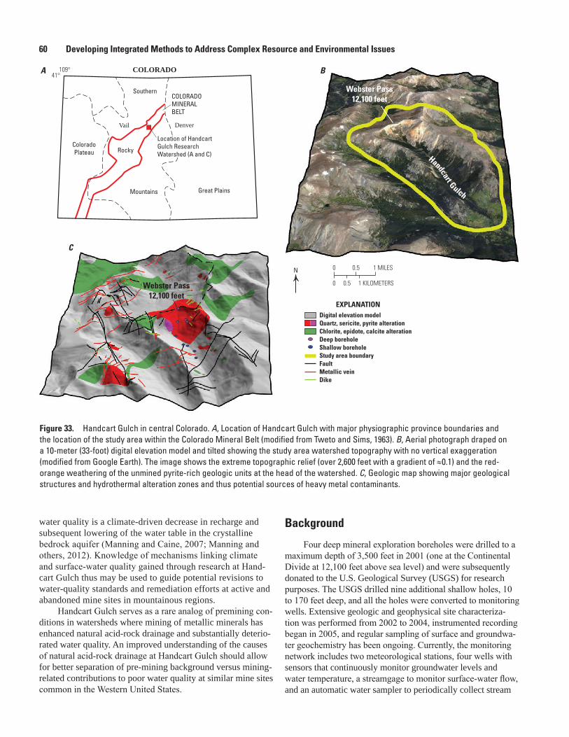
60 Developing Integrated Methods to Address Complex Resource and Environmental Issues
water quality is a climate-driven decrease in recharge and subsequent lowering of the water table in the crystalline bedrock aquifer (Manning and Caine, 2007; Manning and others, 2012). Knowledge of mechanisms linking climate and surface-water quality gained through research at Hand-cart Gulch thus may be used to guide potential revisions to water-quality standards and remediation efforts at active and abandoned mine sites in mountainous regions.
Handcart Gulch serves as a rare analog of premining con-ditions in watersheds where mining of metallic minerals has enhanced natural acid-rock drainage and substantially deterio-rated water quality. An improved understanding of the causes of natural acid-rock drainage at Handcart Gulch should allow for better separation of pre-mining background versus mining-related contributions to poor water quality at similar mine sites common in the Western United States.
Background
Four deep mineral exploration boreholes were drilled to a maximum depth of 3,500 feet in 2001 (one at the Continental Divide at 12,100 feet above sea level) and were subsequently donated to the U.S. Geological Survey (USGS) for research purposes. The USGS drilled nine additional shallow holes, 10 to 170 feet deep, and all the holes were converted to monitoring wells. Extensive geologic and geophysical site characteriza-tion was performed from 2002 to 2004, instrumented recording began in 2005, and regular sampling of surface and groundwa-ter geochemistry has been ongoing. Currently, the monitoring network includes two meteorological stations, four wells with sensors that continuously monitor groundwater levels and water temperature, a streamgage to monitor surface-water flow, and an automatic water sampler to periodically collect stream
Figure 33. Handcart Gulch in central Colorado. A, Location of Handcart Gulch with major physiographic province boundaries and the location of the study area within the Colorado Mineral Belt (modified from Tweto and Sims, 1963). B, Aerial photograph draped on a 10-meter (33-foot) digital elevation model and tilted showing the study area watershed topography with no vertical exaggeration (modified from Google Earth). The image shows the extreme topographic relief (over 2,600 feet with a gradient of ≈0.1) and the red-orange weathering of the unmined pyrite-rich geologic units at the head of the watershed. C, Geologic map showing major geological structures and hydrothermal alteration zones and thus potential sources of heavy metal contaminants.
A
C
Webster Pass12,100 feet
B
Webster Pass12,100 feet
Handcart Gulch
N
0 0.5 1 KILOMETERS
0 0.5 1 MILES
Shallow boreholeDeep borehole
Study area boundary
EXPLANATIONDigital elevation modelQuartz, sericite, pyrite alterationChlorite, epidote, calcite alteration
FaultMetallic veinDike
COLORADO109°41°
COLORADOMINERALBELT
DenverVail
Mountains
Southern
Rocky
Great Plains
ColoradoPlateau
Location of HandcartGulch ResearchWatershed (A and C)

Minerals, Energy, and Climate 61
water for chemical analysis. Results have been previously pub-lished in Caine and others (2006), Manning and Caine (2007), Kahn and others (2008), Verplanck (2008), Verplanck and oth-ers (2008, 2009), and Bove and others (2012).
Results, Conclusions, and Ongoing Work
We have characterized the geology of Handcart Gulch through innovative mapping, collection of rock geochemical and mineralogical data from surface outcrops and drill cores, and direct geophysical imaging of the borehole walls. These data help to characterize the three-dimensional distribution of different types of rocks and minerals in the subsurface, includ-ing minerals that potentially serve as sources of acid-rock drainage, and information on fractures and faults that control groundwater flow. Water-table elevations and their seasonal variations, aquifer test results, subsurface thermal data, and aqueous geochemical and isotopic data (including dissolved gas measurements and groundwater ages) have provided an understanding of aquifer characteristics and hydrological dynamics in the watershed (Manning and Caine, 2007). This understanding of the groundwater system was combined with meteorological data and streamflow measurements to develop a preliminary water budget for the watershed that includes estimates of total precipitation, potential evapotranspiration, streamflow, and groundwater outflow below the stream (Kahn and others, 2008). Two different computer models simulate groundwater flow and thermal processes in the watershed and serve to integrate our current knowledge of the system (Man-ning and others, 2004; Kahn and others, 2008).
Ongoing work at Handcart Gulch includes refinement of our conceptual model of acid-rock drainage and its causes as well as development of new computer models that simulate geochemical processes. Preliminary geochemical modeling has led us to hypothesize that the flow of oxygen from the atmo-sphere into the subsurface is of primary importance in control-ling acid-rock drainage. Recently developed high-technology sensors have been deployed for a variety of novel measure-ments of dissolved oxygen in subsurface air and groundwater to test this hypothesis. Ongoing work also includes continued monitoring of meteorological, hydrological, and geochemical conditions to build a continuous, long-term record. This record is being used to identify changes in water quantity and qual-ity through time and understand processes that control these changes in alpine watersheds. In particular, this record will allow us to evaluate climate variability and potential relations among climate, water quantity, and quality.
Collaborators
This research is funded by the U.S. Geological Survey Mineral Resources and Mendenhall Postdoctoral Fellowship Programs. The work is done in cooperation with the U.S. For-est Service, the Colorado Geological Survey, and the Univer-sity of Colorado, Boulder.
References Cited
Bove, D.J., Caine, J.S., and Lowers, H.A., 2012, Geologic and mineralogic controls on acid and metal-rich rock drainage in an alpine watershed, Handcart Gulch, Colorado: U.S. Geological Survey Scientific Investigations Report 2012–5067, 121 p.
Caine, J.S., Manning, A.H., Verplanck, P.L, Bove, D.J., Kahn, K.G., and Ge, Shemin, 2006, Well construction information, lithologic logs, water level data, and overview of research in Handcart Gulch, Colorado—An alpine watershed affected by metalliferous hydrothermal alteration: U.S. Geological Survey Open-File Report 2006–1189, 14 p., http://pubs.usgs.gov/of/2006/1189/.
Kahn, K.G., Ge, Shemin, Caine, J.S., and Manning, A.H., 2008, Characterization of the shallow groundwater system in an alpine watershed—Handcart Gulch, Colorado, USA: Hydrogeology Journal, v. 16, p. 103–121.
Lins, H.F., Hirsch, R.M., and Kiang, Julie, 2010, Water—The Nation’s fundamental climate issue—A white paper on the U.S. Geological Survey role and capabilities: U.S. Geo-logical Survey Circular 1347, 9 p., http://pubs.usgs.gov/circ/1347.
Manning, A.H., and Caine, J.S., 2007, Groundwater noble gas, age, and temperature signatures in an alpine water-shed—Valuable tools in conceptual model develop-ment: Water Resources Research, v. 43, W04404, DOI: 10.1029/2006WR005349, 16 p.
Manning, A.H., Caine, J.S., Verplanck, P.L., Bove, D.J., and Landis, G.P., 2004, Insights into groundwater flow in an alpine watershed provided by a coupled heat, mass, and fluid transport model, Handcart Gulch, Colorado [abs.]: Geological Society of America Abstracts with Programs, v. 36, p. 539.
Manning, A.H., Todd, A.S., Verplanck, P.L., and Caine, J.S., 2012, Possible links between climate change and deteriorat-ing water quality in a mineralized watershed [abs.]: Geo-logical Society of America Abstracts with Programs, v. 44, no. 7, p. 340.
Todd, A.S., Manning, A.H., Verplanck, P.L., Crouch, Caitlin, McKnight, D.M., and Dunham, Ryan, 2012, Climate-change-driven deterioration of water quality in a mineral-ized watershed: Environmental Science and Technology, v. 46, no. 17, p. 9324–9332.
Tweto, Ogden, and Sims, P.K., 1963, Precambrian ancestry of the Colorado Mineral Belt: Geological Society of America Bulletin, v. 74, p. 991–1014.
Verplanck, P.L., ed., 2008, Understanding contaminants associated with mineral deposits: U.S. Geological Survey Circular 1328, 96 p.

62 Developing Integrated Methods to Address Complex Resource and Environmental Issues
Precipitation Evapotranspiration
WATERSHEDDIVIDE
Recharge
Shallow flow
Baseflow
Regionalflow
BEDROCKAQUIFER
Totalstreamflow
Watertable
Aquiferpermeability (k)
k1 > k2
k2
k1
C D
BA
Figure 34. Watershed approach is used to understand the processes controlling water availability and water quality. A, Using a watershed approach (mass input – mass output = 0), water, and potential contaminants in it, can be tracked and accounted for as it moves from headwater to lowland regions, where ultimately it is used for domestic and industrial purposes. The fundamental source of water is precipitation, in mountainous regions usually in the form of snow. B, Meteorological stations provide measurements of annual precipitation and other data used to monitor longer term climate variability. Wind speed and duration, humidity, solar insolation, and ground temperatures are also measured and provide data used to estimate evapotranspiration—a critical and difficult parameter to measure. C and D, A network of deep and shallow wells is instrumented with water-level and temperature sensors providing hourly hydraulic-head data and its response to variations in recharge. E and F, Geological mapping and characterization of faults and fractures at the surface and in the subsurface using, G and H, borehole geophysical logging are critical to understanding the physical vessel in which groundwater flows. I, The composition of different rock types and how they are altered by hydrothermal fluids imparting potential contaminants such as heavy metals is determined

Minerals, Energy, and Climate 63
E F
G
H
by mineralogical and elemental chemical analyses of drill core samples. J, Hydraulic aquifer tests are used to determine the permeability and storage capacity of bedrock aquifers, which tends to decrease with depth. K, Age and chemistry of groundwater are measured annually in the monitoring well network. L, Stream flow, also known as discharge, is a critical variable for understanding the amount of water that leaves a watershed and is measured at a streamgage. M, Stream-water quality is measured by its chemistry and temperature. M and N, Water quality is measured at benchmark sites annually and at numerous downstream sites during studies where a nonreactive tracer is injected into the stream. O, All data cited above are integrated using sophisticated computer models that allow the quantification of the mass balance and contaminant transport from the watershed. These data and model results also provide opportunities for other research scientists and students to better understand hydrogeological processes, climate, and the unseen subsurface. (USGS photographs)

64 Developing Integrated Methods to Address Complex Resource and Environmental Issues
K
L
I J

Minerals, Energy, and Climate 65
Figure 34. Watershed approach is used to understand the processes controlling water availability and water quality. A, Using a watershed approach (mass input – mass output = 0), water, and potential contaminants in it, can be tracked and accounted for as it moves from headwater to lowland regions, where ultimately it is used for domestic and industrial purposes. The fundamental source of water is precipitation, in mountainous regions usually in the form of snow. B, Meteorological stations provide measurements of annual precipitation and other data used to monitor longer term climate variability. Wind speed and duration, humidity, solar insolation, and ground temperatures are also measured and provide data used to estimate evapotranspiration—a critical and difficult parameter to measure. C and D, A network of deep and shallow wells is instrumented with water-level and temperature sensors providing hourly hydraulic-head data and its response to variations in recharge. E and F, Geological mapping and characterization of faults and fractures at the surface and in the subsurface using, G and H, borehole geophysical logging are critical to understanding the physical vessel in which groundwater flows. I, The composition of different rock types and how they are altered by hydrothermal fluids imparting potential contaminants such as heavy metals is determined by mineralogical and elemental chemical analyses of drill core samples. J, Hydraulic aquifer tests are used to determine the permeability and storage capacity of bedrock aquifers, which tends to decrease with depth. K, Age and chemistry of groundwater are measured annually in the monitoring well network. L, Stream flow, also known as discharge, is a critical variable for understanding the amount of water that leaves a watershed and is measured at a streamgage. M, Stream-water quality is measured by its chemistry and temperature. M and N, Water quality is measured at benchmark sites annually and at numerous downstream sites during studies where a nonreactive tracer is injected into the stream. O, All data cited above are integrated using sophisticated computer models that allow the quantification of the mass balance and contaminant transport from the watershed. These data and model results also provide opportunities for other research scientists and students to better understand hydrogeological processes, climate, and the unseen subsurface. (USGS photographs)—Continued
O
NM
EXPLANATIONStreamInflowsBedrock wells
4.5
4.0
3.5
3.0
2.50 500 1,000
Distance downstream, in meters
BW1 BW2 BW3 BW4 BW5
2,0001,500
pH

66 Developing Integrated Methods to Address Complex Resource and Environmental Issues
Verplanck, P.L., Manning, A.H., Kimball, B.A., McCleskey, R.B., Runkel, R.L., Caine, J.S., Adams, Monique, Gemery-Hill, P.A., and Fey, D.L., 2008, Ground- and surface-water chemistry of Handcart Gulch, Park County, Colorado, 2003–2006: U.S. Geological Survey Open-File Report 2007–1020, 31 p.
Verplanck, P.L., Nordstrom, D.K., Bove, D.J., Plumlee, G.S., and Runkel, R.L., 2009, Naturally acidic surface and ground waters draining porphyry-related mineralized areas of the Southern Rocky Mountains, Colorado and New Mexico: Applied Geochemistry, v. 24, p. 255–267.
Background
The two major forms of carbon (carbon reservoirs) in mine waste are mineral carbon and organic carbon. Mineral carbon includes primary (originally present in the ore/host rock) and secondary (formed after ore rock was left as mine waste) carbonate minerals such as calcite (CaCO3) or magne-site (MgCO3). Where limestone is the ore host rock, primary carbonate minerals are abundant. In the waste rock, physical separation of ore from the host rock during mining resulted in enrichment of sulfide mineral waste relative to carbonate host rock. Over time, buffering of acid (produced via sulfide mineral weathering) by the carbonate minerals results in the destruction of the carbonates. In most other mine wastes (not hosted by carbonates), secondarily formed carbonate minerals are generally lacking.
Organic carbon in mine wastes results from decaying or live vegetation that has been preserved within the pile since emplacement (Stanton, 1999). Photosynthetic plants and other macroorganisms that grow on waste piles are varied but may include fungi, mosses, and vascular plants and grasses. How-ever, the number of any of these organisms on a single waste pile is usually limited, and because mine wastes tend to be highly oxidizing environments, little organic matter is pre-served over time. As surficial plant life is usually sparse, often the decaying or live plant material is removed by mechanical means, such as wind and water erosion.
Microbial carbon, a subset of the organic carbon reser-voir, is difficult to measure and depends upon physical loca-tion of the mine waste, pile composition, types of microbiota (algae versus bacteria), and even the method used to estimate this parameter (Lehmann and others, 2011). Blue-green bac-teria can develop a thick microbial mat on mine waste during wet periods of the year and impart high organic content to the mine waste, but these samples are not always representative of the entire pile. In general, waste piles in low-altitude temper-ate settings tend to have higher microbial masses and num-bers because of readily available water and nutrients. Wastes located above timberline or in deserts are lower in microbial numbers because of harsher environmental conditions (tem-perature and lack of liquid water most months). Other bacteria are present in waste piles, for example thiobacilli (Stanton and others, 2007), which oxidize iron and sulfur and “fix” carbon for cell growth from carbon dioxide in the environment. Num-bers and cell mass of some bacteria can be estimated with dif-ferent tests, but many bacteria are considered “unculturable” because exact growth conditions are unknown and cannot be replicated outside the waste-pile environment. Again, mea-surement of microbial carbon is difficult to obtain on a routine basis because of the variability of populations.
Anthropogenic carbon (for example, support ties and mine timbers) is often present in waste piles. This extraneous carbon still may play a role in sorbing metals or contributing to improved conditions for microbial or plant growth. Numer-ous fungi, mosses, and lichens have been observed growing on timbers in many waste piles. These simpler organisms are
Overview of Carbon Reservoirs and Sequestration in Sulfide Mine Wastes
By Mark R. Stanton and Douglas B. Yager
Issue and Scope
Sulfide mine wastes can be continuous sources of metal contaminants and acidity in local environments. Compared to most soils, sulfide mine wastes are barren with respect to dif-ferent forms of carbon (carbon reservoirs). The acidic charac-ter and high metals content of mine waste-derived water and soil inhibits plant growth and soil development and subsequent carbon sequestration (retention). Changing the geochemical character of these mine wastes may lead to reduced genera-tion of acidity and metals and improved carbon sequestration. In turn, if carbon retention is improved, an organic soil might be able to develop within the mine waste and ultimately result in desirable reductions in metal and acid release and physical stabilization of a waste pile. We are examining methods to alter the geochemistry of mine waste that might make it more chemically inert to weathering and more amenable to carbon sequestration and soil formation.
Objectives
The objectives of this task are to characterize the carbon content of sulfide mine wastes and to see if induced changes in geochemistry (especially pH) can influence carbon seques-tration properties and the quality of water produced by the mine waste. One goal is to see if improvements in the carbon sequestration of mine wastes might lead to enhanced soil formation and thus, potentially reduce acid drainage genera-tion. What is ultimately sought is a chemically and physically stable environment that is less toxic to vegetation and other soil-inhabiting species (for example, fungi).

Minerals, Energy, and Climate 67
“pioneers” that break down complex organic matter to provide more-usable forms of carbon and growth factors to allow growth of various organisms.
Results and Conclusions
We ran some experiments designed to determine if any processes or conditions might lead to sequestration of different forms of carbon and thus increase the total carbon reservoir in mine wastes. The first type of experiment examined addition of biochar (pyrolyzed biomass produced in controlled tem-perature and oxygen conditions) to mine wastes. Recent work with biochar has shown promise in enhancing soil fertility, improving soil drainage, reducing metal toxicity, and main-taining pH at levels best suited for plant growth (Lehmann and others, 2011). The most immediate effect of biochar addition to wastes is the adsorptive removal of metals from solution. High metal concentrations that normally would be present in the absence of char are lowered to more acceptable (nontoxic) levels. Future experiments are aimed at longer term results, for example, determining if biochar provides any increased buffering capacity or increase in soil fertility.
Another type of experiment examined the addition of acid neutralizing capacity (ANC) rocks containing CaCO3 to mine waste. A control run where pure fine-grained limestone was mixed into mine waste on a 1:1 mass basis resulted in the pH being buffered to values above 8.0 (from an initial pH value of 3.4 for mine waste alone). This higher pH not only resulted in lower aqueous metals concentrations but also resulted in the formation of abundant iron oxides, which can adsorb or coprecipitate metals from solution.
Similarly, volcanic rocks that contained minor (<18 weight percent) amounts of CaCO3, plus numerous silicates, were added to mine-waste rocks then reacted in aque-ous solution. The added volcanic rocks (propylitically altered pyroxene andesite; Yager and others, 2008) did produce an increase in pH from 3.4 up to 5.8., Though not as effective as pure limestone, these volcanic rocks do have the ability to neutralize some of the acid drainage that would normally form by reaction of mine waste with water.
As noted, one consequence of raising pH above approx-imately 5.0 was the formation of abundant iron oxide in the reaction vessel (fig. 35). The iron precipitates preferentially formed in the calcite-bearing rock that had relatively higher pH (up to 6.0) than the overlying mine waste (pH=3.4). When iron oxides precipitate from solution, they tend to coprecipitate other metals and even organic matter and con-tinue to adsorb metals and organics after formation. Thus, the process of iron-oxide formation and maintenance of higher pH should be useful in reducing the mobility of toxic metals in the waste pile and in localizing more organic matter within non-sulfide rocks.
Some experiments were carried out where thiobacilli were added to mine waste to see if these might enhance carbon sequestration. Initially, higher numbers of cells were observed but not maintained, and eventually, cell numbers returned to the
original low values. Thus, it was uncertain if the bacteria were able to grow and add mass to the organic carbon reservoir at slightly elevated pH (≤5.8). Any future studies would involve adding heterotrophic bacteria that utilize organic matter and grow more quickly than iron oxidizers to see if they would enhance retention of organic (bacterial) carbon in the waste pile.
We also examined the formation of secondary carbon-ate minerals as a means of raising pH, but these solids appear to be limited in most sulfide mine wastes. That is, results from field work and lab experiments indicate that second-ary carbonate minerals that form in waste piles are unstable (short-lived). If pH is not maintained at higher values (>5.5), the minerals can be redissolved by acid drainage. In addition, the dominant evaporite minerals in most sulfide wastes are sulfate salts of widely varying compositions. These minerals readily redissolve and release stored acidity back to the mine waste, further inhibiting formation of stable carbonate phases. Addition of carbonate (limestone) from outside sources may improve geochemistry of mine wastes, but formation of car-bonate minerals within the waste-pile solids or solutions does not appear to be great enough to have any significant effect on pH or carbon forms.
Figure 35. Formation of iron oxide on acid neutralizing capacity (ANC) rock surfaces in reaction vessel; mine waste material is the upper light-tan layer. The pH of the mine waste solution is 3.4, and the pH of the ANC solution is 5.8. (USGS photograph)

68 Developing Integrated Methods to Address Complex Resource and Environmental Issues
References Cited
Lehmann, Johannes., Rillig, M.C., Thies, Janice, Masiello, C.A., Hockaday, W.C., and Crowley, David, 2011, Biochar effects on soil biota—A review: Soil Biology and Biochem-istry, v. 43, p. 1812–1836.
Stanton, M.R., 1999, The role of weathering in the redis-tribution of trace metals in the Mayday Mine dump near Silverton, Colorado: 4th International Conference on Acid Rock Drainage (ICARD), May 2000, Denver, Colo., p. 1501–1509.
Stanton, M.R., Yager, D.B., Fey, D.L., and Wright, W.G., 2007, Formation and geochemical significance of iron bog deposits, chap. E14 of Church, S.E., von Guerard, Paul, and Finger, S.E., eds., Integrated investigations of environmen-tal effects of historical mining in the Animas River water-shed, San Juan County, Colorado: U.S. Geological Survey Professional Paper 1651, p. 689–720.
Yager, D.B, Choate, L.D., and Stanton, M.R., 2008, Net acid production, acid neutralizing capacity, and associated mineralogical and geochemical characteristics of Animas River watershed igneous rocks near Silverton, Colorado: U.S. Geological Survey Scientific Investigations Report 2008–5063, 63 p.
Metals Sequestration by Biochar in Sulfide-Bearing Mine-Waste Leachate Experiments—Implications for Mine-Waste Reclamation and Carbon Sequestration
By Douglas B. Yager and Mark R. Stanton
Issue and Scope
Sequestration of metals by biochar (pyrolyzed biomass produced in controlled temperature and oxygen conditions) is not well understood but is a potentially important process that could aid in mine-waste reclamation (Fellet and others, 2011). Sulfide-bearing mine waste is a challenging reclamation envi-ronment and can remain devoid of vegetation for decades; the acidic conditions produced by weathering of sulfide minerals prevent re-colonization. Acidity and leaching of metals from barren mine waste can adversely impact local groundwater and surface-water quality and can be a long-term source of con-taminants. Controlled laboratory studies are needed to address the acid neutralizing and metals sequestration potential of biochar. When biochar is applied in the field at mine sites and reclamation areas, there will likely be numerous geoenviron-mental variables that may complicate interpretation of field experiments. Controlled laboratory vessel tests completed as part of this study will help to quantify the metals sequestration potential of biochar and aid in identifying key processes that may influence the effectiveness of biochar applied in field tri-als that cover large areas and involve complex systems.
Objectives
The objective of this study was to determine the acid neu-tralizing capacity and metals sequestration potential (species and quantity) of biochar. In order to simulate natural weather-ing processes in the field, laboratory reaction vessels were constructed that involved leaching (with deionized water) mine waste containing polymetallic veins and host rocks with base metal sulfides (copper-lead-zinc-cadmium, aluminum, and iron), amended with layered or mixed biochar. A goal was to determine the metals sorption capacity, pH, specific conduc-tance, and electrical properties of biochar during laboratory vessel-test reactions.
Background
Hard rock metal mining produces large volumes of mine waste that lack vegetation, organic carbon, and soil nutrients (Yager and others, 2010). Measured soil enzyme activities have also been determined to be very low (Yager and others

Minerals, Energy, and Climate 69
2007, 2010; Yager, Burchell, and others, 2008) indicating poor soil quality. Enhanced recovery of mine waste using soil amendments including biochar and locally sourced rocks having acid neutralizing capacity (ANC) could be a useful reclamation approach in improving soil quality.
Previous leachate and laboratory vessel tests by Stan-ton and Yager (this volume), Yager and others (2009) and Yager, Choate, and Stanton (2008) have addressed the ANC of propylitically altered bedrocks that are commonly associ-ated with mineralized polymetallic vein and porphyry sys-tems. The ANC of these materials was calculated to be high (>20 kilograms CaCO3 [calcium carbonate]/ton equivalent) and metals contribution due to leaching was determined to be low compared with metals contributed from leaching of sul-fide-bearing mine waste (Yager, Choate, and Stanton, 2008). The use of locally sourced ANC rock that could be amended to mine waste during all phases of a project may initially reduce acidity of mine waste upon initiation of mining, reduce recla-mation efforts once mining ceases, aid soil recovery (fig. 36), and lower the carbon footprint of a project due to the reduced need to transport limestone (the traditional remediation mate-rial) to the mine site from long distances.
The use of biochar in mine waste reclamation is in its pioneering stages with field trials only having been recently initiated (Peltz and others, 2010). Degraded mine-waste lands could benefit from application of biochar (Lehmann and oth-ers, 2003). This is due to physical and chemical properties of biochar that make it useful as a soil conditioner to improve soil quality and to sorb inorganic contaminants. In previous studies, biochar was shown to enhance plant growth by sup-plying and retaining nutrients, increase pH and soil moisture retention, improve soil structure, increase nutrient retention,
decrease N2O (nitrous oxide) and CH4 (methane) emissions, sorb metals, and reduce leaching (Lehmann, and others, 2006; Cao and others, 2009; Spokas and others, 2009; Sohi, 2010; Fellet and others, 2011). Biochar is a porous and permeable medium that has a high cation exchange capacity and, once amended to soils and stored in soil aggregates, is recalcitrant to weathering for millennia (Deluca and Aplet, 2008) (fig. 37). It is thus proposed as a potentially effective agent to offset atmospheric CO2 (carbon dioxide) emissions (Yager, Burchell, and others, 2008; Woolf and others, 2010). The laboratory vessel tests completed as part of this project will augment long-duration field trials where biochar is used to reclaim mine waste and other degraded soils.
Results and Conclusions
Laboratory vessel tests were designed to evaluate the physical and chemical reactions of mine-waste leachate with (a) biochar only and (b) a mixture of biochar and mine-waste material. The experiment (a) that isolated biochar only involved saturating 12 centimeters of biochar with pure deionized water. Biochar feedstock was from pine wood, pyrolyzed at 450 °C (degrees Celsius). Nonreacted biochar metal concentrations were analyzed by inductively coupled plasma–mass spectroscopy (Lamothe and others, 2002) for comparison with post-reaction analytical results. Biochar was applied at a 10-percent rate to the vessel involving a biochar mine-waste mixture. Multiple regenerated cellulose mem-brane bags containing biochar were seeded in each vessel for extraction during various phases of reaction. Each vessel was
Figure 36. Acid neutralizing capacity (ANC) rock aiding vegetation and soil recovery of mine waste. Red line is interface between altered andesite lava containing calcite that helps neutralize acidity generated from sulfide-bearing mine waste. Location is near Engineer Pass, at Hough Mine site, San Juan Mountains, Colorado. (Photograph from Alison Burchell, NTS Group).
Mine waste ANC rock
Vegetation
Figure 37. Scanning electron microscope, secondary electron image of pine wood biochar produced by Biochar Engineering Corporation, Niwot, Colorado, using a two-stage, low-temperature pyrolysis unit. Image shows the porous texture and high-surface area of the material. (Image from Sharon Diehl and U.S. Geological Survey microbeam facility in Denver, Colorado. White scale bar [lower right] represents 250 microns.)

70 Developing Integrated Methods to Address Complex Resource and Environmental Issues
Figure 38. Scanning electron microscope, backscatter image of pine-wood biochar exposed to mine-waste leachate in vessel test. Bright areas along cell walls and adjacent to circular areas (plant stoma) adsorbed iron, aluminum, and zinc during reaction in the vessel. Example spectra for bright areas (lower left). Instrument operating conditions were 20 kiloelectron volts (keV); image size is approximately 2 microns across. (Image from Sharon Diehl and U.S. Geological Survey microbeam facility in Denver, Colorado.)
Zn
ZnFe
FeMnCa
S
SAl
C
keV
coun
ts
O
instrumented to measure pH, specific conductance, resistivity, and self-potential. Biochar was analyzed for metals throughout the experiment duration. Preliminary results of vessel tests suggest that base metal cations are sorbed to biochar particles having high surface areas and high cation exchange capac-ity. Scanning electron microscope analyses of biochar reacted with mine-waste leachate shows sorption of iron, aluminum, copper, and zinc by biochar (fig. 38). Longer duration (several months) vessel tests are needed to determine the quantity and species of metals sequestered and whether acidity and specific conductance are reduced over the long term. Future vessel tests will evaluate whether the combined use of ANC rocks and biochar as amendments to mine waste is more effective in sequestering metals and reducing acidity.
Collaborators
Alison Burchell, NTS Group, P.O. Box 3671, Boulder, CO, 80307Carleton Bern, U.S. Geological Survey, PO Box 25046, MS 964D, Denver Federal Center, Denver, CO, 80225.Ted Dodge, Jefferson Watershed Council, P.O. Box, 585, Pony, MT, 59747
Selected References
Burchell, Alison, Yager, D.B., Johnson, R.H., Aiken, J.R., and Butler, Kenna, 2010, High total organic soil carbon (TOSC), low dissolved organic carbon (DOC), and black carbon (BC) horizons, San Juan Mountains, Colorado—Implications for enhanced natural terrestrial carbon sequestration (NTS) land use management and reclamation protocols [abs.]: Geological Society of America Abstracts with Programs, vol. 42, no. 5, p. 160.

Minerals, Energy, and Climate 71
Cao, Xinde, Ma, Lena Qiying, Gao, Bin, and Harris, Willie, 2009, Dairy-manure derived biochar effectively sorbs lead and atrazine: Environmental Science and Technology, v. 43, p. 3285–3291.
DeLuca, T.H., and Aplet, G.H., 2008, Charcoal and carbon storage in forest soils in the Rocky Mountain West: Fron-tiers in Ecology, v. 6, no. 1, p. 18–24.
Fellet, G., Marchiol, L., Vedove, G.D., and Peressotti, A., 2011, Application of biochar on mine tailings—Effects and perspectives for land reclamation: Chemosphere, v. 83, issue 9, p. 1262–1267.
Lamothe, P.L., Meier, A.M., and Wilson, S.A., 2002, The determination of forty-four elements in aqueous samples by inductively coupled plasma–mass spectrometry, in Taggart, J.E., Jr., ed., Analytical methods for chemical analysis of geologic and other materials: U.S. Geological Survey Open-File Report 02–0223–H, p. H1–H11.
Lehmann, Johannes, da Silva, J.P., Jr., Steiner, Christoph, Nehls, Thomas, Zech, Wolfgang, and Glaser, Bruno, 2003, Nutrient availability and leaching in an archeological Anthrosol and a Ferralsol of the Central Amazon basin: fertilizer, manure and charcoal amendments: Plant and Soil, v. 249, p. 343–357.
Lehmann, Johannes, Gaunt, John, and Rondon, Marco, 2006, Bio-char sequestration in terrestrial ecosystems—A review: Mitigation and Adaptation Strategies for Global Change, v. 11, p. 403–427.
Peltz, Christopher, Nydick, Koren, Fitzgerald, Gretchen, and Zillich, Cathleen, 2010, Biochar for soil remediation on abandoned mine lands [abs.]: Geological Society of America Abstracts with Programs, v. 42, no. 5, p. 85.
Sohi, S.P., Krull, E., Lopez-Chapel, E., and Bol, R., 2010, A review of biochar and its use and function in soil: Advances in Agronomy, v. 105, p. 47–82.
Spokas, K.A., Koskinen, W.C., Baker, J.M., and Reicosky, D.C., 2009, Impacts of woodchip biochar additions on greenhouse gas production and sorption/degradation of two herbicides in Minnesota soil: Chemosphere, v. 77, p. 574–581.
Yager, D.B., 2008, Environmental rock properties at aban-doned mine lands that generate or neutralize acid drainage, Silverton, Colorado, chap. K of Verplanck, P.L., ed., Under-standing contaminants associated with mineral deposits: U.S. Geological Survey Circular 1328, p. 64–69.
Yager, D.B., Burchell, Alison, and Johnson, R.H, 2010, A geologic and anthropogenic journey from the Precambrian to the new energy economy through the San Juan volcanic field, in Morgan, L.A., and Quane, S.L., eds., Through the generations—Geologic and anthropogenic field excursions in the Rocky Mountains from modern to ancient: Geologi-cal Society of America Field Guide 18, p. 193–237.
Yager, D.B., Burchell, Alison, and Johnson, R.H., 2008, The Natural terrestrial carbon sequestration potential of Rocky Mountain soils derived from volcanic bedrock [abs.]: Eos, Transactions of the American Geophysical Union, Fall Meeting, Supplement, Abstract GC21A–0172.
Yager, D.B., Burchell, Alison, Robinson, Rob, Odell, Stepha-nie, Dick, R.P., Johnson, C.A., Hidinger, Jack, and Rathke, David, 2007, Natural terrestrial sequestration potential of high plains prairie to subalpine forest and mined-lands soils derived from weathering of Tertiary volcanics [abs.]: EOS, Transactions of the American Geophysical Union, Fall Meeting, Supplement, Abstract B23D–1,588.
Yager, D.B., Choate, LaDonna, and Stanton, M.R., 2008, Net acid production, acid neutralizing capacity, and asso-ciated mineralogical and geochemical characteristics of Animas River watershed igneous rocks near Silverton, Colorado: U.S. Geological Survey Scientific Investigations Report 2008–5063, 63 p.
Yager, D.B., Stanton, M.R., Choate, L.M., and Burchell, Ali-son, 2009, Acid neutralizing capacity and leachate results for igneous rocks with associated carbon contents of derived soils, Animas River AML site, Silverton, Colorado, in Barn-hisel, R.I., ed.: American Society for Reclamation Mining and Safety, Lexington, Ky., p. 1662–1697.
Woolf, Dominic, Amonette, J.E., Street-Perrott, F.A., Lehm-ann, Johannes, and Joseph, Stephen, 2010, Sustainable biochar to mitigate global climate change: Nature Commu-nications, 1:56 doi: 10.1038/ncomms1053, 9 p.

Element Cycling, Toxicity, and Health
methods that produce derivative data necessary to quantify contaminant reservoirs on Mancos Shale in the Uncompahgre River watershed (a tributary to the upper Colorado River), to calculate the flux among reservoirs, and to scale results to include all Mancos Shale landscapes in the UCRB.
Objectives
The objectives of our study were three-fold. The first objective was to construct a critical zone model that tracks con-taminants as Mancos weathers to soil (pedogenesis). Different methods in the literature have been used to track contaminant gain, loss, and redistribution within weathering profiles. Bulk density data (Lisa Stillings, U.S. Geological Survey, written commun., 2007) and chemistry (Tuttle and others, 2007) for Mancos samples were used to evaluate the different methods.
The second objective was to develop a method to quanti-tatively inventory contaminants in different reservoirs across different Mancos land-use landscapes (for example, natural, irrigated, and urbanized). Identifying and quantifying contami-nants in each reservoir can be difficult and costly, so the use of operationally defined reservoirs (readily soluble and insoluble reservoirs) was investigated. The techniques were evaluated comparing chemical results from different rock:water ratio extracts of Mancos soil to stream loads (Tuttle and Grauch, 2009) and chemical data from Mancos rainfall simulation experiments (Elliott and others, 2007; Tuttle, unpub. data). Laboratory leaching experiments were designed to measure the potential for the insoluble soil reservoir to continually supply contaminants to the readily soluble soil reservoir as contaminants are removed with drainage.
The third objective was to develop a protocol from con-structing contaminant budgets at the watershed scale. Budgets include contaminant inventories, contaminants solubilized but returned to the soil by infiltration, contaminants transported by runoff, and contaminants in eroded soil and alluvium. The utility of these budgets for scaling data from small studied watersheds to larger regional landscapes was tested using results from the literature and the two studies discussed in the Background section.
Background
The U.S. Geological Survey (USGS) partnered with Federal and State agencies to collect and help understand data on these nonpoint contaminant sources. In 2003, the USGS initiated a large multidisciplinary study on undisturbed Mancos Shale in the Uncompahgre River watershed above the flood plain focusing on weathering of black shale and the impact of recreational land use. Geochemical data were collected on samples from trenches, core, and regional soil surveys. The
Salt and Selenium Cycling in Shale-Derived Soils, Southwestern United States
By Michele L.W. Tuttle, Juli Fahy, and Jean Morrison
Issue and Scope
The Colorado River in the southwestern portion of the United States is considered one of the most stressed in the world because of increasing salinization and selenium (Se) contamination (Engberg, 1999; Serageldin, 2000). Nearly 36 million people and 4.5 million acres of United States and Mexico farmland depend on the Colorado River (U.S. Depart-ment of Interior, 2005) and salinization damages in the United States alone are estimated at $306 million (U.S. Department of Interior, 2005). Rocks weathering in the Upper Colorado River Basin (UCRB) supply a significant portion of the con-taminants. Tuttle and Grauch (2009) estimate that 33 percent of the 2005 solute load in the river near the Colorado-Utah border was derived from chemical weathering of Cretaceous Mancos Shale. The dominant anion in the load was sulfate, and the amount attributed to the Mancos is equivalent to 1,400,800 tonnes per year of gypsum dissolution. Nearly all the Se contamination in the UCRB is from natural weathering and irrigation of the Mancos (Clark, 1995; Engberg, 1999). Tuttle and Grauch (2009) estimated that 60 t a−1 of Se were derived from Mancos Shale landscapes in Colorado, repre-senting nearly the entire 2005 Se load in the river near the Colorado-Utah border. The Se load is of concern because con-centrations in the river exceed the U.S. Environmental Protec-tion Agency’s (EPA) National Recommended Water Quality Criteria (5 micrograms per liter [µg L−1] for freshwater) in some reaches inhabited by threatened and endangered species of fish (Hamilton, 1998), and Se impacts the habitat of other wildlife along the river such as waterfowl (Presser and others, 1994; Butler and others, 1996).
Previous studies have described salt and Se in the UCRB; however, none include a comprehensive understanding of the processes that occur during both chemical and mechani-cal weathering of rock and derived soil, nor do they produce geochemical models that describe the flux of salt and con-taminants among rock, soil and alluvium, and aqueous phases. Conceptually and quantitatively understanding contaminant cycling under natural and irrigated conditions is critical for developing strategies to preserve the health of soils developed on shale landscapes across the arid southwest and to remediate salinization and contaminants in waterways that flow through them. The focus of this study was to develop and test different

Element Cycling, Toxicity, and Health 73
Figure 39. Depth profile of Mancos Shale trench showing tau (τ) values for total salt (gypsum equivalent, [GE]) and selenium (Se) in soil, transition soil, and shale. mg/kg, milligrams per kilogram.
results of this study show that weathering processes redistrib-ute and concentrate contaminants in secondary reservoirs. On undisturbed landscapes, most redistributed contaminants are stored in the soil and, even during severe storm events, are only transported short distances. In a parallel study by the Bureau of Reclamation and Natural Resources Conservation Service, similar Mancos data were collected from irrigated fields and adjacent vacant land on the Uncompahgre River flood plain. The results of this study showed that irrigation from farming and other anthropogenic activities mobilized large concentra-tions of stored salt and Se into streams and groundwater.
Although the data from both studies were collected and analyzed with similar methods, no attempt was made to integrate them into an understanding of how Mancos Shale weathers under different land-use practices. To achieve this, contaminants in different reservoirs need to be quantified and the flux of contaminants among reservoirs determined. This study developed the methods to integrate the data, provides documentation on how to construct contaminant cycles in this and similar watersheds, and provides tools for land managers to assess the impact of contaminants from weathering land-scapes under different land-use scenarios.
Results and Conclusions
Tracking contaminant mobility.—Index elements (gener-ally titanium [Ti], neodymium [Nd], zirconium [Zr], and silicon dioxide [SiO2]) are commonly used to track the gain or
loss of contaminants during pedogenesis. Using bulk density measurements, Ti was chosen as the least mobile index ele-ment and was used to calculate a Tao (τ) value for each sample in our trench profiles. Tao converts concentration into a frac-tion lost or gained relative to that in the starting material, cor-rects for mass changes of other components during weathering (White, 2003), and is calculated as follows (Brimhall, 1991):
τj,w = (Cj,w/Cj,o)/Ci,w/Ci,o) – 1. (5)
The Cj,w and Cj,o are concentrations of contaminant j (salt or Se) in weathered and starting material, respectively, and Ci,w/Ci,o are the concentrations of the immobile, index phase i (Ti) in weathered and starting material. Tao depth profiles for salt and Se (fig. 39) show an 18-fold increase in salt in the soil zone and a small net loss of Se over the profile. The salt accumulation zone forms because nearly 90 percent of the rainfall and all of the snowmelt infiltrates into the soil where the moisture is subsequently lost through evapotranspiration leaving behind the salt. Selenium increases slightly in this salt accumulation zone.
Availability of contaminants.—Multiple rock:water extract data showed that extract salinity is controlled by gypsum solu-bility and that smaller ratios (higher water amounts) extracted more salt and Se. Our goal was to use an extract ratio that best mimicked natural conditions, so the extract data were compared to data from rain simulation experimental (RSE) data collected in the field. The concentration of Se in the saturation paste
–1–1 –0.5 0 0.5 1–500
–400
–300
–200
–100
0
Dept
h in
cen
timet
ers
5 10 15 20
Transition
Soil
Shale
EXPLANATION
τSalt(GE) τSe(total)

74 Developing Integrated Methods to Address Complex Resource and Environmental Issues
Figure 40. Salt and selenium extract (ex) concentrations (dry weight basis) in sequential saturation paste extracts. mg/kg, milligrams per kilogram.
Table 3. Total and extractable selenium and salt (gypsum equivalent) inventories for Mancos Shale soil (0–45 centimeters) in the Uncompahgre River watershed. Values are totals for the landscape (in metric tonnes [t]) and per square meter (m–2) of landscape. Undisturbed landscapes are those above the flood plain (FP).
[g, gram; km2, square kilometers; Se, selenium; nonirr., nonirrigated; --, no data]
LandscapeUndisturbed 470 km2 FP Irrigated 119 km2 FP nonirr. 101 km2 FP wetland 18 km2
Total Extractable Total Extractable Total Extractable Total ExtractableSe (g m–2) 0.8 0.05 1.5 0.01 2.5 0.09 7.2 0.7Se (t) 380 26 180 1.2 250 9.3 130 12Salt (g m–2) 2.2 x 10⁴ 870 -- 630 -- 2.1 x 10³ -- 3.2 x 10³
Salt (t) 1.0 x 10⁷ 4.1 x 10⁵ -- 7.5 x 10⁴ -- 2.1 x 10⁵ -- 5.7 x 10⁴
Table 4. Fluxes calculated from precipitation rates, rainfall simulation data, and saturation-paste-extract data are compared to loads measured in tributaries and the Uncompahgre River (UR). Calculated budget for tributaries include the undisturbed Mancos Shale above the flood plain (FP).
[-, no data; %, percent; g acre–1, grams per acre]
Salt (g acre–1) Selenium (g acre–1)
Sources Water loads% URload
Calculated budget
% URload
Water budget
% URload
Calculated budget
% URload
Precipitation 2.1 x 10⁸ <1 -- 5.7 x 10⁴ <1 -- --River above study 9.3 x 10¹⁰ 31 -- 0 0 -- --Diversion (irrigation) 8.5 x 10¹⁰ 28 -- 0 0 -- --Tributaries in study 2.1 x 10¹⁰ 7 2.0 x 10¹⁰ 7 1.8 x 10⁵ 5 1.4 x 10⁵ 4Mancos soils (FP) 7.2 x 10¹⁰ 24 8.3 x 10¹⁰ 24 3.2 x 10⁶ 95 3.5 x 10⁶ 96Irrigated -- -- 7.3 x 10¹⁰ 21 -- -- 3.0 x 10⁶ 82Nonirrigated -- -- 1.0 x 10¹⁰ 3 -- -- 4.9 x 10⁵ 14Other soils (FP) 2.7 x 10¹⁰ 10 -- -- 0 0 -- --Uncompahgre River 3.0 x 10¹¹ 100 -- -- 3.4 x 10⁶ 100 3.6 x 10⁶ --
0
0.005
0.01
0.015
0.02
0.025
0.03
1 2 3 4 5 6 7 8 9 10
Sequential extract number
Se(e
x) m
g/kg
soi
l
500
1,000
1,500
2,000
Salt(
ex) m
g/kg
soi
l

Element Cycling, Toxicity, and Health 75
extract (SPE) was 5.0 µg L–1 compared to 5.6 µg L–1 in the RSE runoff. The SPE overestimates the salt content; however, this was not an issue on a watershed scale. These results indicate that soil SPE concentrations are a good estimation of read-ily soluble reservoirs and provide reliable data for calculating fluxes between reservoirs. Results from our leaching experi-ments (fig. 40) show a continual supply of contaminants to the soluble reservoir controlled by adsorption and solubility.
Contaminant inventories and fluxes.—Salt and Se inventories (table 3) were constructed using regional soil data collected in the two studies mentioned above. Mancos Shale landscapes on the Uncompahgre River flood plain contain more Setotal per square meter than undisturbed Mancos landscapes above the flood plain. Irrigated fields contain the least amount of extractable Se and salt due to leaching over time but are still serious nonpoint contaminant sources as determined from the leaching experiments. Fluxes from dif-ferent reservoirs are calculated from SPE and inventory data. Comparison of the calculated fluxes with measured stream loads is given in table 4.
The authors are applying these methods to a study in a sec-ond upper Colorado River tributary (Pariette Draw, Utah) where Tertiary shale (Green River and Uinta Formations) weathers under the same conditions as in the Mancos Shale study. The Tertiary shale contributes salt and Se (plus boron) to the stream in concen-trations that exceed EPA Total Maximum Daily Load standards.
Collaborators
Collaborators in the Mancos Shale study are Bureau of Land Management, Montrose Colorado; USGS Colorado Water Science Center; and Bureau of Reclamation. Collabo-rators in the ongoing Pariette Draw study are Bureau of Land Management, Vernal and Salt Lake City, Utah; Colorado River Salinity Control Program (Bureau of Reclamation); Bureau of Land Management Salinity Program; Utah Divi-sion of Water Quality; Utah State University; and Kansas State University.
References Cited
Brimhall, G.H., Lewis, C.J., Ford, Chris, Bratt, James, Taylor, Gordon, and Warin, Oliver, 1991, Quantitative geochemical approach to pedogenesis—Importance of parent material reduction, volumetric expansion, and eolian influx in lateri-tization: Geoderma, v. 51, p. 51–91.
Butler, D.L., Wright, W.G., Steward, K.G., Campbell Osmundson, Barbara, Krueger, R.P., and Crabtree, D.W., 1996, Detailed study of selenium and other constituents in water, bottom sedi-ment, soil, alfalfa, and biota associated with irrigation drainage in the Uncompahgre Project Area and in the Grand Valley, west-central Colorado, 1991–93: U.S. Geological Survey Water-Resources Investigation Report 96–4138, 136 p.
Clark, S.L., 1995, The distribution of selenium in the upper Colorado River: Tempe, Arizona State University, Ph.D. dis-sertation, UMI 9526987, Ann Arbor, UMI Company, 150 p.
Elliott, J.E., Herring, J.R., Ingersoll, G.P., Kosovick, J.J., and Fahy, Juli, 2007, Rainfall-runoff and erosion data from the Mancos Shale Formation in the Gunnison Gorge National Conservation Area, southwestern Colo-rado, 2003–2006: U.S. Geological Survey Open-File Report 2007–1002–G, 67 p., at https://pubs.er.usgs.gov/publication/ofr20071002G/.
Engberg, R.A., 1999, Selenium budgets for Lake Powell and the upper Colorado River: Journal of the American Water Resources Association, v. 35, p. 771–786.
Hamilton, S.J., 1998, Selenium effects on endangered fish in the Colorado River Basin, in Frankenberger, W.T., Jr., and Engleberg, R.A., eds., Environmental chemistry of sele-nium: New York, Marcel Dekker, Inc., p. 297–313.
Presser, T.S., Sylvester, M.A., and Low, W.H., 1994, Bioac-cumulation of selenium from natural geologic sources in Western States and its potential consequences: Environmen-tal Management v. 18, p. 423–436.
Serageldin, Ismail, 2000, World’s rivers in crisis—Some are dying; others could die: World Commission on Water for the 21st Century, at http://www.worldwatercouncil.org/Vision/6902B03438178538C125683A004BE974.htm.
Tuttle, M.L., and Grauch, R.I., 2009, Salinization of the upper Colorado River—Fingerprinting geologic salt sources: U.S. Geological Survey Scientific Investigations Report 2009–5072, 62 p., at http://pubs.usgs.gov/sir/2009/5072/.
Tuttle, M.L.W., Fahy, Juli, Grauch, R.I., Ball, B.A., Chong, G.W., Elliott, J.G., Kosovich, J.J., Livo, K.E., and Stillings, L.L., 2007, Results of chemical analyses of soil, shale, and soil/shale extract from the Mancos Shale Formation in the Gunnison Gorge National Conservation Area, Southwestern Colorado, and at Hanksville, Utah: U.S. Geological Open-File Report 2007–1002–D, 24 p., at http://pubs.usgs.gov/of/2007/1002/D/.
U.S. Department of Interior, 2005, Quality of water, Colorado River Basin progress report no. 22: Denver, Colo., Bureau of Reclamation, 69 p., at http://www.usbr.gov/uc/progact/salinity/index.html.
White, A.F., 2003, Natural weathering rates of silicate miner-als, in Holland, H.D., and Turekian, K.K., eds., Treatise on geochemistry, vol. 5: New York, Elsevier, p. 133–168.

76 Developing Integrated Methods to Address Complex Resource and Environmental Issues
Microbial Communities Involved in Arsenic and Iron Cycling at the Lava Cap Mine Superfund Site, California
By Andrea L. Foster
Issue and Scope
Understanding the spatial and temporal relations among microbial groups in field and laboratory settings is required for (1) process-based understanding of the role and impact of microorganisms on toxic trace metal mobility and bioavail-ability, (2) the development of microbially enhanced remedia-tion technologies, and (3) development of microbially based processes to extract economically important elements from mineral deposits. The U.S. Environmental Protection Agency (EPA) Superfund Program, which is in charge of hazardous waste sites at which human health has been determined to be particularly at risk, has a specific directive to pursue “green” and “renewable” technologies developed from materials at or near the site. Native microorganisms that are found to perform a useful function could, in theory, be used to help clean up hazardous waste sites.
Objectives
Our objective was to evaluate the feasibility for native, iron-oxidizing microbes to be used in passive bioreactors to help remove arsenic (As) from water at the Lava Cap Mine Superfund Site (LCMS), California (fig. 41). Over a 2-year period, we conducted geochemical and microbiological monitoring studies at several locations on the site where the iron-oxidizing microbial communities were observed to form visible colonies. Our specific actions were (1) to quantify the seasonal and spatial variation in the magnitude of As uptake by biogenic ferric (hydr)oxide, (2) to determine the composi-tion of the microbial community producing the ferric (hydr)oxide, (3) to track seasonal and spatial variation in the compo-sition of that community, (4) to monitor the performance of a naturally occurring passive bioreactor developed fortuitously at the base of an intact tailings dam, and (5) to determine the mechanism of As sequestration on the biogenic ferric hydr(oxide) and its reversibility.
Background
The Lava Cap Mine exploited a gold-bearing quartz-carbonate-vein system typical of the Sierran (“Lode”) Gold Belt. Peak production at the Lava Cap occurred between 1934 and 1943 when about 90,000 tons of ore per year were processed (Clark, 1970). To facilitate removal of the gold and accessory sulfide minerals, the ore was crushed to a very fine
sand or silt grain size for processing. The Lava Cap Mine and surrounding area were placed on the EPA National Priority (that is, Superfund) List of priority sites for cleanup due to several factors that coalesced in December 31, 1996, when a log-tailings retention dam failed at the mine site sending an estimated 8,000–10,000 cubic meters of tailings down a stream and into a second, intact tailings dam that was being used as a small private lake by local residents. Between 1996 and 2000, members of the U.S. Geological Survey (USGS) Mineral Resources Program worked with the California Department of Toxic Substances Control to characterize the degree to which the catastrophic log-dam failure and mine-tailings release affected downstream waterways (specifically Little Clipper Creek and Lost Lake) in terms of (1) metals loading to sediments and waters and (2) the extent of As transformation from forms in sulfide minerals originally in the tailings to labile and oxidized forms (Foster and others, 2011). During the course of this research, the investigators discovered that aquatic flocculent ferric (hydr)oxide deposits were biogenic in nature, and that these deposits scavenged As from water (Foster and Ashley, 2002). The EPA took inter-est in this work and, beginning in 2006, funded the USGS to study these communities in greater detail.
Results and Conclusions
Major conclusions from the study (which employed genetic, culturing, chemical, and spectroscopic techniques) are as follows:1. The site-wide average As concentration in dried biogenic
ferric (hydr)oxide (BFH) was >10,000 milligrams per kilogram (mg/kg; ppm [parts per million]) but ranged from 3,000 to 39,000 mg/kg (fig. 42). Typical As concen-trations in LCMS tailings range from 500–1000 mg/kg, demonstrating the efficacy of this biosorbent in accumu-lating arsenic.
2. BFH contains far more iron (Fe) and manganese (Mn) than As (average of 29 percent and 10 percent, respec-tively; fig. 42), and therefore is useful for lowering the concentration of these “nuisance” elements from water. This is particularly advantageous because after removal of As, in a pilot cleanup plant, discharge from the site was still above water-quality standards for Fe and Mn.
3. A naturally occurring passive bioreactor developed at the site removed an average of 44, 55, and 29 percent of As, Fe, and Mn, respectively, from water over the 2-year sampling period (fig. 43). Variability in performance was related to water-flow rate rather than changes in influent As concentration, with lower flow resulting in greater As, Fe, and Mn removal.
4. Both arsenate and arsenite are accumulated by BFH, and As is both adsorbed and co-precipitated on BFH. Analysis of synchrotron-based X-ray absorption spectra allowed these conclusions to be made. Purely adsorbed

Element Cycling, Toxicity, and Health 77
Figure 41. Regional to site-level overview of the Lava Cap Mine Superfund Site, Nevada County, California. An estimated 10,000 cubic meters (m3) of tailings were released into Little Clipper Creek due to failure of a tailings dam (labeled) located near the mine. Most of this material settled in the downstream deposition area and in Lost Lake—a second tailings retention structure that already contained an estimated 382,277 m3 of tailings deposited during the active mining period. Interaction of water with tailings produces conditions conducive to the growth of iron-oxidizing microbial communities; these are most extensively developed in water seeping out below the Lost Lake dam.
IDAHO-MARYLAND ROAD
GREENHORN MOUNTAIN ROAD
LAVA CAP MINE(CENTRAL SHAFT)
BANNER MINE
LostLake
Drainage tunnel
TAILINGSDAM
TAILINGSDAM
Clip
per C
reek
LittleClipper
Creek
GreenhornLittle
Creek
Wolf Creek
Little Deer Creek
20 21 22
151617
272829
32 33 34
2345
T.16N.
T.15N.
R. 9 E.
2800
2800
2800
2800
2800
3000
2800
3000
3200
28003000 2800
3200
3200
2800
3000
3200
3600
3800
3400
2600
2800
3000
3200
2600
2600
2600
2600
2400
2400
39°15'
38°12'30"
121°00' 120°57'30"
0 0.5 KILOMETERS
0 0.5 MILES
LittleGreenhorn
Creek
NevadaCity
GrassValley
SR49
SR49
SR20
SR174
Deer
Creek
ROLLINS
RESERVOIR
ClipperCreek
MAP AREA
Base map USGS Chicago Park quadrangle, scale 1:24,000.Modified from Foster and Ashley (2002).

78 Developing Integrated Methods to Address Complex Resource and Environmental Issues
species are associated only with the surfaces of minerals, whereas co-precipitated species are also located within the bulk mineral. Adsorbed species can be released from minerals by small changes in solution composition such as pH or ionic strength changes.
5. The microbial consortia producing BFH are of low diversity. They appear to be dominated by species of the Leptothrix genus of Eubacteria. Analysis of DNA extracted from fresh BFH flocs across the LCMS show a remarkable similarity and low diversity of the microbial community. Under the microscope (light and electron), BFH is seen to be composed primarily of microbial sheaths, which are coated with ferric (hydr)oxide (fig. 44). Few sheath-forming bacteria exist in nature, and fewer still prefer environments low in carbon (so called “oligotrophic” environments). These unique characteristics allowed the identification of members of the genus Leptothrix as the predominant members of the BFH-forming microbial community.
6. Native populations of suboxic to anoxic bacteria are present in BFH from the LCMS; these bacteria can dissolve ferric (hydr)oxide and release to solution some or all of the As, Fe, or Mn associated with it. The BFH produced by Leptothrix and other community mem-bers has the potential to be “food” for another group of microorganisms—the iron-reducing bacteria (FeRB). These bacteria have several different strategies for coupling the reduction of ferric iron to energy-generating processes, and they have been the focus of many stud-ies. No gene for iron reduction has yet been discovered that would allow an estimation of the abundance of the FeRB community by gene-based techniques. Therefore, most probable number (MPN), a serial-dilution, culture-based technique, was employed to assess the abundance of FeRB in the BFH. Substantial populations of FeRB were enumerated suggesting that if a passive bioreactor were constructed, careful maintenance of the geochemi-cal environment in the reactor would be required to ensure that As was not being re-released under changing seasonal conditions.
Our study found that naturally occurring, Leptothrix-dominated microbial communities could remove As to below water-quality criteria in a natural system analogous to a pas-sive bioreactor, but removal is highly dependent on flow rate and therefore would need to be carefully managed. Both major species of arsenic bind to iron hydroxide precipitated on the sheaths of Leptothrix in what appears to be predominantly adsorbed complexes that may be easily removed by changes in pH or concentration of competing anions such as phosphate or silica. Although the communities are dominated by Leptothrix and appear to change little with season, a latent population of iron-reducing bacteria is also present and poses a threat to the long-term stability of the solid-phase arsenic. Simple changes in geochemical conditions could mobilize a significant fraction of arsenic bound to Leptothrix sheaths. However, this problem
Figure 42. Basic statistics of arsenic (top), iron, and manganese dry weight concentrations measured over the study period at several locations at the Lava Cap Mine Superfund Site.
5,000
0
10,000
15,000
30,000
Arse
nic,
mill
igra
ms
per k
ilogr
am
20,000
25,000
0
20
40
Iron,
in p
erce
nt
10,000
0
20,000
30,000
40,000
50,000
60,000
70,000
Man
gane
se, m
illig
ram
s pe
r kilo
gram
Biogenic ferric (hydr)oxide samples Algae

Element Cycling, Toxicity, and Health 79
Figure 43. Percent attenuation of dissolved arsenic (As), iron (Fe), and manganese (Mn) through a naturally developed passive bioreactor system that was measured several times during the study period as the difference between the dissolved concentrations of these elements measured at site LL1 (where low oxygen [O2], Fe-, Mn-, and As-rich water seeps out below the dam) and site LL10 (just upstream of the site where seep water meets highly oxygenated lake water from the dam spillway). Most of the variability in removal of the constituents can be traced to differences in water-flow conditions, where higher flow rate equals less removal of the three constituents.
Figure 44. Dual-transmitted-light and epifluorescent-light image (400×) of cells of a sheath-forming, iron-oxidizing bacterium (L. ochracea) that composes the bulk of the biogenic ferric (hydr)oxide produced at the Lava Cap Mine Superfund Site. Members of the genus Leptothrix prefer low-carbon environments, are aerobic, and have the ability to form sheaths, which is relatively rare among the bacteria. Members of the genus are known to harbor proteins on their sheaths and capsular material that enzymatically oxidize iron and manganese. The cells have been stained with propidium iodide for visibility under ultraviolet light demonstrating their filamentous nature and the fact that very few sheaths are populated—another well-known characteristic of L. ochracea (Foster and Ashley, 2002).
10
20
30
40
50
60
70
80
90
100
June October November
Perc
ent
February2006 2007 2008
Date
March August October March
EXPLANATIONAsFeMn
LL1 LL10
LostLake

80 Developing Integrated Methods to Address Complex Resource and Environmental Issues
is analogous to the current problem of disposal of large vol-umes of chemically prepared As adsorbed on iron hydroxides produced in active remediation systems. In those remediation systems, the potentially labile adsorbed As is currently man-aged by maintaining this material under oxidizing, subaqueous conditions in lined holding ponds (Paktunc and others, 2003).
Collaborators
U.S. Environmental Protection Agency Region 9, Superfund Section through interagency agreement DW14-95571901-0.Stanford University Environmental Molecular Sciences Institute (National Science Foundation grant)
References Cited
Clark, W.B., 1970, Gold districts of California: California Division of Mines and Geology Bulletin 193, 186 p.
Foster, A.L., and Ashley, R.P., 2002, Characterization of arse-nic species in microbial mat communities in the vicinity of the Lava Cap gold mine, Nevada City, CA: Geochemistry: Exploration, Environment, and Analysis, v. 2, p. 253–261.
Foster, A.L., Ashley, R.P., and Rytuba, J.J., 2011, Arsenic spe-cies in weathering tailings and biogenic solids at the Lava Cap Mine Superfund Site, Nevada County, CA: Geochemical Transactions, v. 12, p. 1-21, doi:10.1186/1467-4866-12-1.
Paktunc, Dogan, Foster, Andrea, and Laflamme, Gilles, 2003, Speciation and characterization of arsenic in Ketza River mine tailings using X-ray absorption spectroscopy: Envi-ronmental Science & Technology, v. 37, p. 2067–2074.
Geochemical Signatures as Natural Fingerprints
By Bronwen Wang and Robert Seal
Issue and Scope
The migration of Tanner crabs (Chionoecetes bairdi) throughout their life cycle is poorly understood but could have important implications for fisheries management. Relatively dense populations of juvenile Tanner crabs have been found in several areas within Glacier Bay, Alaska; these could be nursery areas from which maturing crabs disperse.
Objectives
Our objectives were to evaluate if geochemical sig-natures are imparted to the carapace during molt or to the muscle tissue during growth and, if so, to determine if they could serve as a natural fingerprint that identifies the area where molting or growth occurred. Geochemical signatures may reflect subtle elemental or isotopic compositional dif-ferences that arise from hydrologic, geologic, or nutritional variations in Glacier Bay (fig. 45).
Background
Elemental and isotopic variations in biota arise from dif-ferences in local environmental conditions. In some instances, these “geochemical fingerprints” are sufficiently unique to serve as life-history markers. Geochemical fingerprints have been used to distinguish stock and migration patterns for a variety of fish and marine invertebrates (Edmond and others, 1989; DiBacco and Levin, 2000). Stable isotopic studies have been carried out on a variety of topics related to aquatic and terrestrial ecosystems (Fry and Sherr, 1984; Carmichael and others, 2004). Environmental conditions that may result in unique geochemical signatures include food source, carbon source (for example, shelf or oceanic), salinity and tempera-ture differences, and differences in the local geology.
The success of geochemical fingerprinting tools in other studies (that is, DiBacco and Levin, 2000) led us to consider the possibility that such signatures in Tanner crabs may aid in understanding their migration within Glacier Bay. Tanner crab life-history characteristics make them well suited for a geochemical fingerprinting approach. Female Tanner crabs do not molt again after they molt to sexual maturity. Therefore, if a female Tanner crab leaves the area where she molted to maturity (for example, a nursery area), the geochemical sig-nature in her carapace could be used as a marker for the area in which she molted. In addition, isotopic variations in the muscle tissue could serve as an indicator of crab movement and thus could complement the geochemical information

Element Cycling, Toxicity, and Health 81
from the carapace. For example, if crabs leave the nursery area after molting, the carapace should reflect the signature of the nursery area, whereas the muscle may reflect both the terminal molt and a more recent environment. Based on the geological and hydrological heterogeneity present in Glacier Bay (fig. 46) and the life history of the Tanner crab, there is a reasonable chance geochemical variations imparted to the crab body tissue can be used to determine the area where the terminal molt occurred.
Results and Conclusions
Elemental and isotopic differences were found in crabs collected from the five locations within Glacier Bay, and it appears promising that a geochemical fingerprint of location of molt may be identified (fig. 47; Wang and others, 2007).
To fully evaluate the potential of geochemical finger-printing as a tool in understanding crab movement within Glacier Bay, more work is necessary to examine the stability of the elemental and isotopic signature with time, changes of the isotopic signature with diet, isotopic signature of different prey types, the possibility of sex as a confound-ing factor, and the role of biogenic calcite on the elemental signature and isotopic signatures through separation of the calcite and chitin.
Such work would have management application in area-based fisheries management (for example, marine protected areas and essential fish habitat designation) that requires an increased understanding of spatial processes, such as rearing areas and movement during the course of an organisms development. Long-term movements of juvenile Tanner crabs are very difficult to quantify because tags that can be reliably retained through the molt have not been developed. Movement of females and sublegal males cannot be detected in traditional tagging studies that use fisheries to recapture tagged animals based on sex and size regulations of the fishery. Multi-year sonic tagging studies are expensive and relatively few animals can be tracked. If geochemical fingerprinting can eventually be used to determine movement with ontogeny, it will be an elegant, robust, relatively cost-effective tool that can achieve results in a short period of time (that is, one survey as opposed to several years of sonic tracking).
Collaborators
Spencer Taggart and Jennifer Mondragon, U.S. Geological Survey, Juneau, AK
Figure 45. Collection and sample preparation of Tanner crabs from Glacier Bay National Park. A, Tanner crab collection, B, carapace, and C, meat during sample preparation. (USGS photographs)
A B
C

82
Developing Integrated Methods to Address Com
plex Resource and Environmental Issues
WachusettInlet
ScidmoreBay
CharpentierInlet
BartlettCove
HughMiller
ALASKA
135°30'136°00'136°30'137°00'137°30'
58°30'
59°00'
Mineral occurrence within study area
Au
Fe, Ni?
Ag, Au
CuCu, NiCu, MoPb, ZnZnAg, Au, CuMoAg
FeMo, W
Ag, Cu, Pb
Cu, Fe, Ti
Ag, Pb, Zn
Pb, Zn
Sampling locations within bays
Snow and iceSedimentary rocksMagmatic rocksMetamorphic rocks
EXPLANATION
0 1 KILOMETERS
0 1 MILES
Base map from Geiselman and others (1997).
Figure 46. Sampling locations relative to generalized bedrock geology, and the locations of known mineral occurrences within Glacier Bay National Park.
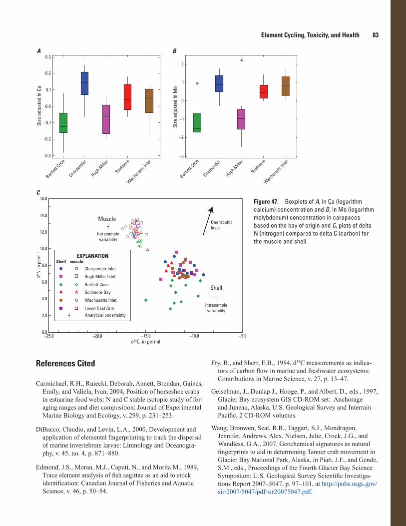
Element Cycling, Toxicity, and Health 83
Figure 47. Boxplots of A, ln Ca (logarithm calcium) concentration and B, ln Mo (logarithm molybdenum) concentration in carapaces based on the bay of origin and C, plots of delta N (nitrogen) compared to delta C (carbon) for the muscle and shell.
0.0
2.0
4.0
6.0
8.0
10.0
12.0
14.0
16.0
–25.0 –20.0 –15.0 –10.0 –5.0δ13C, in permil
δ15N
, in
perm
il
Charpentier Inlet
Hugh Miller Inlet
Bartlett Cove
Scidmore Bay
Wachusetts Inlet
Lower East ArmAnalytical uncertainty
Shell muscle
Shell
Intrasamplevariability
Muscle
Intrasamplevariability
One trophiclevel
EXPLANATION
0.3
0.2
0.1
0.0
–0.1
–0.2
–0.3
Bartlett C
ove
Charpentier
Hugh Mille
r
Scidmore
Wachusetts
Inlet
Size
adj
uste
d ln
Ca
A
2
1
0
–1
–2
–3
Bartlett C
ove
Charpentier
Hugh Mille
r
Scidmore
Wachusetts
Inlet
Size
adj
uste
d ln
Mo
B
C
References Cited
Carmichael, R.H., Rutecki, Deborah, Annett, Brendan, Gaines, Emily, and Valiela, Ivan, 2004, Position of horseshoe crabs in estuarine food webs: N and C stable isotopic study of for-aging ranges and diet composition: Journal of Experimental Marine Biology and Ecology, v. 299, p. 231–253.
DiBacco, Claudio, and Levin, L.A., 2000, Development and application of elemental fingerprinting to track the dispersal of marine invertebrate larvae: Limnology and Oceanogra-phy, v. 45, no. 4, p. 871–880.
Edmond, J.S., Moran, M.J., Caputi, N., and Morita M., 1989, Trace element analysis of fish sagittae as an aid to stock identification: Canadian Journal of Fisheries and Aquatic Science, v. 46, p. 50–54.
Fry, B., and Sherr, E.B., 1984, d13C measurements as indica-tors of carbon flow in marine and freshwater ecosystems: Contributions in Marine Science, v. 27, p. 13–47.
Geiselman, J., Dunlap J., Hooge, P., and Albert, D., eds., 1997, Glacier Bay ecosystem GIS CD-ROM set: Anchorage and Juneau, Alaska, U.S. Geological Survey and Interrain Pacific, 2 CD-ROM volumes.
Wang, Bronwen, Seal, R.R., Taggart, S.J., Mondragon, Jennifer, Andrews, Alex, Nielsen, Julie, Crock, J.G., and Wandless, G.A., 2007, Geochemical signatures as natural fingerprints to aid in determining Tanner crab movement in Glacier Bay National Park, Alaska, in Piatt, J.F., and Gende, S.M., eds., Proceedings of the Fourth Glacier Bay Science Symposium: U.S. Geological Survey Scientific Investiga-tions Report 2007–5047, p. 97–101, at http://pubs.usgs.gov/sir/2007/5047/pdf/sir20075047.pdf.

84 Developing Integrated Methods to Address Complex Resource and Environmental Issues
Trace Metal Partitioning Between Sediments and Groundwater in the Basin-Fill Aquifer Surrounding Fallon, Nevada
By Lisa L. Stillings, Nicole K. Cutler, John K. McCormack, and Ralph L. Seiler
Issue and Scope
There has been relatively little research into the geochemi-cal cycle of tungsten (W) in the environment. This became apparent during investigations into possible environmental causes of a childhood leukemia cluster in Fallon, Nevada. These studies found high concentrations of W in airborne dust, lichens, and in groundwater of the local basin-fill aquifers. An understanding of the processes that govern the occurrence of W in the environment requires knowledge of the speciation of W within solid phase minerals. The purpose of this research was to identify the spatial variation, concentration, and mineralogi-cal phase association(s) of W and other trace metals commonly found in the basin-fill aquifer surrounding Fallon, Nevada.
Objectives
A thorough description of hydrogeochemical conditions in the basin-fill aquifer is key to understanding W and trace metal geochemical cycles in the study area. Water and sediment samples were collected from the same depth in the aquifer in order to evaluate the geochemical controls on solid and aque-ous phase composition. The overall focus of the entire study is to address the hypotheses that redox levels in the aquifer will control the solid-solution partitioning and mineral phase association of W and other trace metals. Seiler and others (2005) proposed that Eh-pH conditions in groundwater of the basin-fill aquifers would promote reductive dissolution of iron and manganese oxyhydroxides thereby releasing adsorbed W into solution. The first objective of the study is to document the geochemistry and mineralogy of sediments in the basin-fill aquifer and to describe the solid phase partitioning of W and trace metals between the sediment fractions. Trace elements of interest include those that form oxyanions (W, molybdenum [Mo], chromium [Cr], arsenic [As], and uranium [U]) and cobalt (Co).
Background
The current debate over the sources and sinks of W in the Carson Desert of Nevada began with investigations by the Centers for Disease Control and Prevention (CDC) into possible ties between a childhood leukemia cluster and environmental causes in Lahontan Valley, an agricultural area
surrounding the city of Fallon, Nevada. In 2002, the CDC National Center for Environmental Health nominated W for toxicological and (or) fate and transport studies in order to investigate W sources and mobilization mechanisms. Envi-ronmental factors were eventually ruled out as the cause of the leukemia cluster in Fallon after extensive testing of water, soil, air and dust, and jet fuel (Koutsospyros and others, 2006). However, the observations of increased W in tree-core samples, lichens, human blood and urine (CDC, 2003), and groundwater samples (Seiler and others, 2005) have prompted researchers to learn more about the geochemical cycle of W in the environment.
The study area was located in Lahontan Valley where samples of aquifer sediment were collected from five drilling sites near domestic wells that exhibit a wide range of aqueous W concentration. Boreholes were drilled to access water-bearing sediment layers in the shallow (<13 meters (m) depth) and intermediate (≈13–50 m) aquifers. Aquifer sediments were collected with depth, at approximately 6-m intervals or at water-bearing layers, down to a maximum 37-m depth. One sediment sample was collected at the well-screen depth in the shallow aquifer, and four samples were collected at well-screen depth in the intermediate aquifer.
Results and Conclusions
The analytical techniques of scanning electron micros-copy–energy dispersive spectroscopy (SEM–EDS; Goldstein, 2003) and X-ray diffraction (XRD; Bish and Post, 1989) were used to identify sediment mineralogy. Analyses showed that the samples contained quartz, plagioclase feldspar, potassium feldspar, augite, biotite (with titanium substitution), amphibole (hornblende, actinolite, and tremolite), ilmenite, hematite, and calcite. Amorphous iron coatings were identified on many of the grains and were interpreted to be ferric oxyhydroxides. Manganese coatings were only observed in two samples. Pyrite was observed in euhedral, anhedral, framboidal, and crystalline habits and was often observed in samples that contained iron oxides. Less abundant minerals include apatite, barite, calcite, olivine, rhodonite, siderite, sphalerite, and zircon. Diatoms of ≈10–100 micrometer (µm) size, including Surirella sp., and other calcareous microfossils were observed. Tungstate minerals were not detected, nor was W observed with the SEM–EDS while using the backscatter mode.
Solid phase bulk W concentrations range from 1.3 to 7.9 milligrams per kilogram (mg/kg), with an analytical error of 5 percent based on duplicate sample analyses. Other transition metals with chemistries similar to W (Group 6B of the periodic table), Mo and Cr, had bulk chemistry concentra-tions ranging from 0.7 to 33.5 mg/kg and from 8 to 40 mg/kg, respectively. Bulk concentrations of As ranged from 6 to 25 mg/kg, U from 1.4 to 4.5 mg/kg, and Co from 4.6 to 16.1 mg/kg. Bulk W concentrations are positively correlated with bulk Cr, As, U, and Co values in the sediment. Bulk Mo concentrations were variable and did not correlate with bulk W concentrations.

Element Cycling, Toxicity, and Health 85
Table 5. Grain-size analysis.
[%, percent; <, less than; μm, micrometer; mm, millimeter]
Grain size
Sample% clay (<2 μm)
% silt (2–53 μm)
% sand (53 μm–2 mm)
Classification1
CDP39-12.2 19 3 78 sandCDP39-29 3 78 19 sandFCL43-12 7 25 68 sandy siltFCL43-19.8 6 62 32 silty sandFCL43-19.9 6 80 14 sandFCL46-6.1 3 91 6 sandFCL46-24.4 5 91 4 sandFCL54-12.2 2 77 21 sandFCL54-12.3 19 18 62 sandy siltFCL54-13.7 1 74 25 sandFCL54-24.4 1 84 15 sandFCL54-30.5 2 76 22 sandFPo01-6.1 42 4 54 clayey siltFPo01-18.3 17 6 78 siltFPo01-36.6 15 28 56 sandy siltFPo01-36.7 18 31 51 sandy silt
1Size classification from Shepard (1954).
Figure 48. Partitioning of trace elements among seven sediment fractions. Averages are calculated from 16 samples. Exch ions, exchangeable ions; MnOx, manganese oxides; c-FeOx, crystalline iron oxides nc-FeOx, noncrystalline iron oxides; OM, organic matter.
Sediment phases
Extra
ctio
n pe
rcen
tage
0
20
Exch ions
CarbonatesMnOx
nc-FeOxc-FeOx
OMSulfid
es
40
60 EXPLANATIONWMoCrAsUCo

86 Developing Integrated Methods to Address Complex Resource and Environmental Issues
The partitioning of W and trace metals within aquifer sediments was measured with a selective extraction proce-dure (SEP) designed to target the following seven sediment fractions (Amacher, 2003): exchangeable ions, carbonates, manganese oxides (MnO), noncrystalline iron oxides (ncFeO), crystalline Fe oxides (cFeO), organic matter (OM), and sul-fides. Figure 48 compares the percent of each element found within each sediment fraction, where percent is calculated as
percentc
c
i z
i zz
=
=∑
,
,1
7
(5)
where ci = average concentration of element i and z = SEP extraction step. Results indicate that (1) Mo was the only element with a significant percentage of its mass bound in the exchangeable ion fraction; (2) all elements except W associ-ated with carbonates; (3) Mo and As were the only elements to significantly bind with MnO; (4) all elements were present in the ncFeO and cFeO fractions, but W exhibited the highest percentage in each; (5) W was the predominate trace metal to associate with OM; and (6) all elements except W were predominately associated with the sulfide fraction.
Grain size classification (table 5; Shepard, 1954) shows two distinct groups of grain sizes in the sample set: sands and silts. Bulk concentrations of W, Cr, As, U, and Co are significantly higher in the silt samples than in the sand samples. The variabil-ity in bulk Mo concentrations was too great to show statistical difference between the grain sizes. Bulk median concentration of W in silt-size sediments, 5.3 mg/kg, was significantly different from the median concentration in sands, 1.9 mg/kg, as deter-mined by a t-test at P value = 0.009. This observed partitioning of trace elements into the silt-size sediments is due to the chemi-cal composition of the finer grained sediments. From the SEP it was determined that the main sediment phases to host trace ele-ments contained inorganic and organic carbon, Fe, and S. All of these components are present in higher concentrations in the silt-size sediments. Mineralogic composition also varied with grain size. Ferrihydrite, pyrite, and calcite (secondary, precipitated in situ) were only identified primarily in finer grained samples.
In conclusion, no primary tungsten minerals (for example, scheelite) were found in the aquifer sediments. Instead, W, with bulk sediment concentrations of 1.3–7.9 mg/kg, partitioned into three sediment phases: noncrystalline and crystalline iron oxides (together referred to as FeO), and organic matter (OM). The variation in W concentration with grain size is due to increased concentrations of FeO and OM in the smaller size fraction.
Other trace elements (Mo, Cr, As, U, and Co) are found in the aquifer sediments in concentrations ranging from 0.7 to 40 mg/kg. The concentrations of all of these elements, with the exception of Mo, correlate strongly with W concentration. The chemistry of W, however, is unique because, although the other trace metals are found predominately associated with the sulfides in aquifer sediments, W was found primarily in the FeO and OM sediment phases (Cutler and others, 2009).
Acknowledgments
The authors thank the homeowners in Lahontan Val-ley for permission to collect samples on their properties. We thank Paul Lamothe and Monique Adams of the USGS-MRP Analytical Laboratory for analysis of the leachate samples, and Robert Oscarson, USGS, for assistance with SEM. NKC acknowledges funding from a student research grant from the Geological Society of America, and from a USGS Cooperative Agreement, Number G09AC00075, awarded to the University of Nevada, Reno.
Collaborators
Program of Hydrological Sciences and Department of Geological Sciences and Engineering, University of Nevada Reno
References Cited
Amacher, M.C., 2003, Manual of Methods: Open-File Report 2003, USDA Forest Service, Intermountain Research Sta-tion, Forestry Sciences Laboratory, Logan, UT, 62 p.
Bish, D.L., and Post, J.E., eds., 1989, Modern powder diffrac-tion: Mineralogical Society of America Reviews in Mineral-ogy, v. 20, 369 p.
Centers for Disease Control and Prevention (CDC), 2003, Cross-sectional exposure assessment of environmental con-taminants in Churchill County, Nevada: Centers for Disease Control and Prevention, accessed May 20, 2008, at http://www.cdc.gov/nceh/clusters/Fallon/study.htm.
Cutler, N.K., Stillings, L.L., and McCormack, J.K., 2009, Sediment phase associations of tungsten in the alluvial aqui-fers, Fallon, Nevada [abs.]: Geological Society of America, Abstracts with Programs, Vol. 41, No. 7, p. 328.
Goldstein, Joseph, 2003, Scanning electron microscopy and X-ray microanalysis: Kluwer Academic/Plenum Publishers, 689 p.
Koutsospyros, A., Braida, W., Christodoulatos, C., Derma-tas, D., and Strigul, N., 2006, A review of tungsten: From environmental obscurity to scrutiny. Journal of Hazardous Materials v. 136, p. 1–19.
Seiler, R.L., Stollenwerk, K.G., Garbarino, J.R., 2005, Factors controlling tungsten concentrations in ground water, Carson Desert, Nevada: Applied Geochemistry v. 20, p. 423–441.
Shepard, F.P., 1954, Nomenclature based on sand-silt-clay ratios: Journal of Sedimentary Petrology, v. 24, p.151–158.
Element Cycling, Toxicity, and Health 87
Bioaccessibility of Potentially Toxic Metals and Metalloids in Earth Materials
By Suzette A. Morman and Geoffrey S. Plumlee
Issue and Scope
Throughout our lifetime, we are exposed to a variety of soils, mineral dusts, and other earth materials that contain a variety of mineral or metal toxicants. Although we commonly think of contaminants as the result of only anthropogenic processes, natural processes can also concentrate potentially toxic elements with known human health risks such as arsenic, cadmium, and lead in rocks and soils. Both natural (weather-ing and winds) and anthropogenic processes (mining, smelt-ing, and construction) may expose and promote distribution of these naturally occurring contaminants into the environment.
For example, the air we breathe, depending upon the sea-son, where we are, and other factors, can contain a complex mix of airborne particulate matter (PM) derived from many different natural and anthropogenic sources. Although research has sub-stantiated associations between PM exposure and cardiovascular and respiratory disease, it was focused on PM generated from anthropogenic sources. Few studies considered contributions from geogenic PM (produced from the Earth by natural pro-cesses, for example, volcanic ash, windborne ash from wildfires, and mineral dusts) or geoanthropogenic PM (produced from natural sources by processes that are modified or enhanced by human activities, for example, dusts produced from areas that have undergone desertification as a result of human practices).
In addition to inhalation of PM, ingestion can also be a primary pathway for exposure to earth materials such as soils, settled dust deposits, and flood sediments. Although geophagia, the purposeful consumption of soils, is still practiced in some cultures, most ingestion of earth materials is inadvertent. Inadvertent ingestion occurs through hand to mouth transfer, consumption of soil particles on improperly washed produce, or by swallowing of inhaled particles that have been trapped in mucus lining the respiratory tract and cleared into the throat.
Earth materials that are taken up by the body interact chemically with the body’s fluids encountered along the dif-ferent exposure routes (fig. 49). These interactions strongly influence potential toxicity effects. For example some earth materials can contain bioaccessible toxicants that are readily released into the body’s fluids and are available for uptake by the body. Other earth materials can be toxic because they are biodurable (are insoluble in the body’s fluids), can persist in the body for years, and cause long-term toxicity effects.
Under the auspices of the U.S. Geological Survey Miner-als and Health Project, the Development of Mineral Environ-mental Assessment Methodologies Project, and this project,
we have collaborated with numerous colleagues in the earth and public health sciences to measure and interpret toxicologi-cally relevant mineralogical, physical, geochemical, and bio-accessibility characteristics of many different earth materials. By elucidating these characteristics, we can help toxicologists and other public health specialists identify primary exposure routes of concern, how these materials may be taken up by the body, and their chemical behavior and toxicological properties once in the body.
Objectives
This project has helped fund the development of physi-ologically based extraction tests (PBETs), also called in vitro bioaccessibility assessments (IVBAs), which model the solu-bility behavior of diverse earth materials in fluids encountered along inhalation and ingestion exposure routes.
We have modified and adapted several commonly used PBETs covering a variety of simulated body fluid types and have explored their use in estimating exposures to potentially toxic metals in a wide array of naturally occurring earth materi-als and earth materials transformed for use by society. The results allow us to estimate what portion of a sample is soluble or bioaccessible and thus available to the body. The results also allow us to understand how mineralogy and processes such as weathering and transport may alter biosolubility. Through the use of these tests, our Minerals and Health Research Laboratory (see Laboratory Facilities and Capabilities section, this volume) provides valuable information on the solubility or bioaccessibil-ity of elements present in a wide array of earth materials.
Background
Physiologically based extraction tests provide a quick and inexpensive alternative to animal or cell-line test-ing. Bioaccessibility testing was pioneered in the 1970s to explore the solubility of radionuclides in mine wastes and dusts. Since the 1970s, much of the focus has been on the development of PBETs to model the gastric and intestinal bioaccessibility of lead in mine wastes and contaminated soils, and PBETs to model the biosolubility of asbestos and man-made vitreous fibers in fluids lining the respiratory tract. These tests use fluids that are similar in composition and pH to those in the human body to evaluate what percent-age of a metal or other element is soluble and thus available for uptake by the target organs such as the kidneys or liver. Although these tests do not measure the amount the body absorbs (bioavailability), the results are important for under-standing how matrix, mineral, particle size, process, and speciation impact the solubility or bioaccessibility of often poorly understood earth materials.

88 Developing Integrated Methods to Address Complex Resource and Environmental Issues
Results and Conclusions
Controls on metal mobility in soils, such as soil pH, organic carbon content, and absorption by clay minerals, are generally site specific, vary by metal, and may affect bioacces-sibility as well. This is illustrated by our work comparing arse-nic (As) concentrations in simulated gastric fluid extractions of dusts from a playa in the Mojave Desert to those in back-ground soils. The bioaccessibility of As in the dusts, present with evaporative salts, was two to three times higher than we have measured in background soils. This increase is attributed to desorption and concentration of As from ferric oxides that coat silt and clays, whereas the As in soils remains bound.
However, though matrix properties are important, the mineral form of the metal and the pH of the leaching solution also play an important role. For example, fluorosis (a disease marked by severe dental and bone problems) has been noted in livestock and wildlife following some volcanic eruptions and has been attributed to high levels of water-soluble fluoride in volcanic ash; the fluoride is either leached from the ash into water supplies that are then consumed by the animals or is directly taken up by animals that eat ash-coated forage. Water extrac-tion tests are traditionally used to test fluoride release from volcanic ash but have been shown not to adequately predict the development of fluorosis in animals following some types of eruptions. Using a low pH (pH 1.5) simulated gastric PBET
Figure 49. Schematic diagram illustrating exposure pathways and variability in body fluid types and compositions that can be encountered by earth materials (from Plumlee and Ziegler, 2006).
Stomach(pH 1.5, electrolytes,
enzymes)
Large intestine(near-neutral pH, reducing)
Small intestine(near-neutral pH, reducing)
Primary bronchi
Nasal cavity
Oral cavity
Pharynx
Larynx
Trachea
Secondary bronchi
Terminal bronchioles
Alveolar duct, sac,and alveoli
Cilia
Aqueous fluid(near neutral pH, high PO2)
Alveolar macrophage(acidic lysosomal fluids)
Capillary–plasma(pH 7.4, moderately high
PO2, high proteins)
Lung fluid(pH 7.4, high PO2,
mucoproteins, phospholipids)
Mucus(mucoproteins, water)
Interstitial fluids(pH 7.4; high Na,
low K; low proteins)
Intracellular fluids(pH 7.4; high K, Mg, P)
Interstial fluids, plasma(exposed at breaks in skin:
pH 7.4; plasma has high proteins)
Sweat(acidic pH, high urea,
lactic acid, etc.)

Element Cycling, Toxicity, and Health 89
on ash samples from several volcanoes, we demonstrated that the higher pH (pH >5) water extractions may grossly underes-timate the amount of bioaccessible fluoride in some types of volcanic ash (fig. 50).
To elucidate the processes that may alter metal solubil-ity in long traveled dusts such as those from the Sahel region of Africa, we developed a new PBET method to analyze toxicant bioaccessibility in dusts from air filters collected at a source site in Africa as well from downwind locations in the Caribbean. In general, concentrations of elemental toxicants such as As exceeded the U.S. mean background concentra-tion, and bioaccessibility increased downwind along the transect away from the origin in both the simulated gastric and lung fluid extractions.
We have also applied PBETs to examine roadside vegeta-tion exposed to fugitive dusts generated from mining transport vehicles. These tests indicated that the bioaccessibility of lead and other metal toxicants varied by sample and by vegeta-tion type. Bioaccessibility was greatest in vegetation samples for cadmium and zinc, and rinsing produced only moderate decreases that varied by plant type. Lead concentration and bioaccessibility were highest in the dust, likely related to weathering and oxidation, and lowest in the mine concentrate, a sulfide-bearing ore, with low bioaccessibility. This indicates that multiple processes, both biological and physical, may be involved at every site.
Earth scientists have a growing role in helping health scientists anticipate potential health issues associated with
toxic metals and metalloids in diverse natural and anthropo-genic earth materials and understanding the processes that enhance bioaccessibility, such as weathering and transport. In vitro bioaccessibility tests, or PBETs, are a useful assessment tool that can be easily applied to many different types of earth materials. They provide needed insights into how earth materi-als behave chemically in the body and how readily metal or metalloid toxicants may be released from the earth materials and become available for uptake by the body.
Collaborators
U.S. Geological Survey Minerals and Health Project, Richard L. Reynolds, William Brumbaugh, and Virginia Garrison.
Publications Funded in Part by This Project
Brumbaugh, W.G., Morman, S.A., and May, T.W., 2011, Con-centrations and bioaccessibility of metals in vegetation and dust near a mining haul road, Cape Krusenstern National Monument, Alaska: Environmental Monitoring and Assess-ment, v. 182 (1–4), p. 325–340.
Morman, S.A., Garrison, V.H., Plumlee, G.S., Lowers, H.A., and Bunnell, J.E., 2009, Assessing concentration and bioaccessibility of potentially toxic elements in African dust [abs.]: Geological Society of America Abstracts with Programs, v. 41, no. 7, p. 554.
Morman, S.A., and Plumlee, G.S., 2010, In vitro physiologi-cally based extraction tests of volcanic ash from diverse volcanoes [abs]: Cities on Volcanoes 6, Tenerife, Canary Islands, May–June 2010, http://www.ivhhn.org/meetings/pastmeetings.html.
Morman, S.A., Reynolds, R.L., Reheis, Marith, Goldstein, Harland, Plumlee, Geoffrey, and Wolf, R.E., 2008, Bioac-cessibility of toxic elements in dusts from dry saline lakes in the Mojave Desert [abs.]: Geological Society of America Meeting Abstracts with Program, v. 40, no. 6, p. 78.
Figure 50. Total fluoride, simulated gastric fluid (SGF) leach, and water-leach fluoride concentrations for volcanic ash samples.
100,000
10,000
1,000
100
10
1
0.1
Mill
igra
ms
per k
ilogr
am
Oldo
inyo
Leng
ai,
Tanz
ania
(200
7)
Ilam
atep
ec,
El S
alva
dor (
2005
)
Mou
nt S
t. He
lens
,
Was
hing
ton
(198
0)
Hale
ma’
uma’
u,Ha
wai
i (20
08)
EXPLANATIONSGF
Water
Fluoride, total

90 Developing Integrated Methods to Address Complex Resource and Environmental Issues
Diffusive Gradients in Thin Films and Biotic Ligand Models—Tools for Evaluating the Health of the Environment
By Laurie S. Balistrieri
Issue and Scope
Historical mining activities have left a legacy of metal-enriched water and sediment in many watersheds in the United States. A major concern of regulators, land managers, and the public is the potential adverse impact of the met-als on environmental health or, alternately, on the quality of air, water, and sediment and the health of humans, fish, wildlife, and other organisms living in these watersheds. The challenge for U.S. Geological Survey (USGS) scientists is to provide detailed information that links the distribution, behavior, and geochemical characteristics of metals to their availability and toxicity to living organisms. Understanding how geochemical pathways expose biota to metal toxicity is the foundation for other Federal and State agencies to (1) set standards for the quality of air, water, and sediment in the environment; (2) evaluate the best options for cleaning up contaminated sites; or (3) minimize risks of metal toxicity to the health of humans and other organisms.
Objectives
The project goals were to define the geochemical factors and processes that influence the toxicity of metals to aquatic organisms in watersheds affected by historical mining. A com-bination of sampling and modeling tools were used. Concen-trations and chemical forms (or speciation) of dissolved metals were determined using traditional filtering methods, diffu-sive gradients in thin films (DGT), and computer modeling, whereas the health of aquatic organisms was evaluated using concentrations of dissolved metals, water-quality criteria, and biotic ligand models (BLMs). In addition, processes such as transport by water that redistributes metals throughout the environment and geochemical reactions that transform metals among their dissolved and particulate phases were examined.
Each of the study sites had unique geochemical charac-teristics and together they provided information on dissolved metal behavior and toxicity to aquatic organisms for a wide range of environmental conditions. The study sites were as follows:1. Copperas Brook and the Ompompanoosuc River that
drain the Elizabeth Copper Mine Superfund Site in Vermont. Copperas Brook was very acidic (pH <3) and enriched in dissolved metals during the study and flowed into the slightly basic, pristine Ompompanoosuc
River (pH ≈8). The study examined environmental con-ditions and health of aquatic organisms in the mixing and reaction zone just downstream of the confluence of the two rivers.
2. South Fork of the Coeur d’Alene River and its tribu-taries, which flow through the Coeur d’Alene mining district in northern Idaho. Populations of fish are non-existent or limited in these watersheds and appear to be affected by high concentrations of dissolved metal.
3. Silver Bow and High Ore Creeks, which, respectively, drain the Butte mining district and the abandoned Comet Mine in Montana. Diel (24 hour) changes in dissolved metal concentrations occur in these creeks, and an approach for evaluating toxicity to fish was developed for these dynamic systems.
4. Upper Columbia River in northeastern Washington that is downstream of several smelter facilities. The effect of exchange between metal-enriched groundwater and upper Columbia River water on dissolved metal concen-trations was assessed.
Background
Dissolved metal ions exist as free ions, complexes with inorganic anions or ligands (for example, carbonate, chlo-ride, or sulfate), or as complexes with organic ligands, such as fulvic and humic acids. The relative concentrations of these various chemical forms of dissolved metals depend on the composition of the solution. Of importance to studies of environmental health is that chemical speciation of dissolved metals influences their toxicity to aquatic organisms. Gener-ally, free metal ions are considered to be more toxic to aquatic organisms than metal-ligand complexes.
DGT and BLMs are two tools used in our studies to define links among the compositions of natural waters, speciation of dissolved metals, and environmental health. DGT is a sampling method that involves transport by dif-fusion of dissolved metal ions through hydrogel to a resin that binds the free-metal ion. Concentrations of dissolved labile metal, which includes free ions and complexes with inorganic anions as well as some complexes with organic anions, depending on their size and ability to dissociate, are determined. Metals associated with colloidal and particulate phases do not enter the hydrogel because of their size. DGT also provides information about dissolved chemical specia-tion because the diffusion of metal-organic ligand complexes through the hydrogel is slower than diffusion of free ions and metal-inorganic ligand complexes. Therefore, a solu-tion containing dissolved free-metal ions and complexes of metal with inorganic and organic ligands would contain less dissolved labile metal than if the solution had no organic ligands. In addition, DGT samplers continuously accumulate metal during deployment in water. This characteristic pro-vides two advantages. First, low concentrations of dissolved
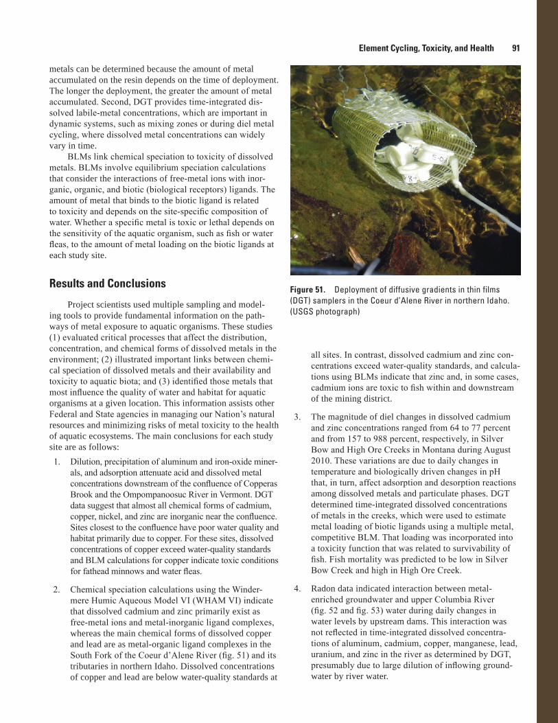
Element Cycling, Toxicity, and Health 91
metals can be determined because the amount of metal accumulated on the resin depends on the time of deployment. The longer the deployment, the greater the amount of metal accumulated. Second, DGT provides time-integrated dis-solved labile-metal concentrations, which are important in dynamic systems, such as mixing zones or during diel metal cycling, where dissolved metal concentrations can widely vary in time.
BLMs link chemical speciation to toxicity of dissolved metals. BLMs involve equilibrium speciation calculations that consider the interactions of free-metal ions with inor-ganic, organic, and biotic (biological receptors) ligands. The amount of metal that binds to the biotic ligand is related to toxicity and depends on the site-specific composition of water. Whether a specific metal is toxic or lethal depends on the sensitivity of the aquatic organism, such as fish or water fleas, to the amount of metal loading on the biotic ligands at each study site.
Results and Conclusions
Project scientists used multiple sampling and model-ing tools to provide fundamental information on the path-ways of metal exposure to aquatic organisms. These studies (1) evaluated critical processes that affect the distribution, concentration, and chemical forms of dissolved metals in the environment; (2) illustrated important links between chemi-cal speciation of dissolved metals and their availability and toxicity to aquatic biota; and (3) identified those metals that most influence the quality of water and habitat for aquatic organisms at a given location. This information assists other Federal and State agencies in managing our Nation’s natural resources and minimizing risks of metal toxicity to the health of aquatic ecosystems. The main conclusions for each study site are as follows:1. Dilution, precipitation of aluminum and iron-oxide miner-
als, and adsorption attenuate acid and dissolved metal concentrations downstream of the confluence of Copperas Brook and the Ompompanoosuc River in Vermont. DGT data suggest that almost all chemical forms of cadmium, copper, nickel, and zinc are inorganic near the confluence. Sites closest to the confluence have poor water quality and habitat primarily due to copper. For these sites, dissolved concentrations of copper exceed water-quality standards and BLM calculations for copper indicate toxic conditions for fathead minnows and water fleas.
2. Chemical speciation calculations using the Winder-mere Humic Aqueous Model VI (WHAM VI) indicate that dissolved cadmium and zinc primarily exist as free-metal ions and metal-inorganic ligand complexes, whereas the main chemical forms of dissolved copper and lead are as metal-organic ligand complexes in the South Fork of the Coeur d’Alene River (fig. 51) and its tributaries in northern Idaho. Dissolved concentrations of copper and lead are below water-quality standards at
all sites. In contrast, dissolved cadmium and zinc con-centrations exceed water-quality standards, and calcula-tions using BLMs indicate that zinc and, in some cases, cadmium ions are toxic to fish within and downstream of the mining district.
3. The magnitude of diel changes in dissolved cadmium and zinc concentrations ranged from 64 to 77 percent and from 157 to 988 percent, respectively, in Silver Bow and High Ore Creeks in Montana during August 2010. These variations are due to daily changes in temperature and biologically driven changes in pH that, in turn, affect adsorption and desorption reactions among dissolved metals and particulate phases. DGT determined time-integrated dissolved concentrations of metals in the creeks, which were used to estimate metal loading of biotic ligands using a multiple metal, competitive BLM. That loading was incorporated into a toxicity function that was related to survivability of fish. Fish mortality was predicted to be low in Silver Bow Creek and high in High Ore Creek.
4. Radon data indicated interaction between metal-enriched groundwater and upper Columbia River (fig. 52 and fig. 53) water during daily changes in water levels by upstream dams. This interaction was not reflected in time-integrated dissolved concentra-tions of aluminum, cadmium, copper, manganese, lead, uranium, and zinc in the river as determined by DGT, presumably due to large dilution of inflowing ground-water by river water.
Figure 51. Deployment of diffusive gradients in thin films (DGT) samplers in the Coeur d’Alene River in northern Idaho. (USGS photograph)

92 Developing Integrated Methods to Address Complex Resource and Environmental Issues
Collaborators
Richard Blank, R.G. Blank Enterprises, LLCStephen Cox, U.S. Geological SurveyChristopher Mebane, U.S. Geological SurveyDavid Nimick, U.S. Geological SurveyBarbara Paul, University of WashingtonNadine Piatak, U.S. Geological SurveyRobert Seal, U.S. Geological SurveyPeter Swarzenski, U.S. Geological Survey
Selected References
Balistrieri, L.S., 2009, Dissolved and DGT labile metal con-centrations—Comparisons among thermodynamic specia-tion models and implications for biotic ligand models [abs.]: Conference on DGT and the Environment, Sardinia, Italy, October 7–9, 2009.
Balistrieri, L.S., and Blank, R.G., 2008, Concentrations of dissolved and labile Cd, Cu, Pb, and Zn in the South Fork Coeur d’Alene River, Idaho—Comparisons among chemi-cal equilibrium models and implications for biotic ligand models: Applied Geochemistry, v. 23, no. 12, p. 3355–3371.
Balistrieri, L.S., and Blank, R.G., 2009, Dissolved and labile concentrations of Cd, Cu, Pb, and Zn in the South Fork Coeur D’Alene River, Idaho—Comparisons among equi-librium models and implications for biotic ligand models [abs.]: American Chemical Society Annual Meeting, Salt Lake City, UT, March 22–26, 2009.
Balistrieri, L.S., Cox, S.E., and Swarzenski, P.W., 2011, Using diffusive gradients in thin films (DGT) to monitor dis-solved labile concentrations of trace elements in the upper Columbia River, WA, USA [abs.]: 2011 Association for the Sciences of Limnology and Oceanography (ASLO) Aquatic Sciences Meeting, San Juan, Puerto Rico, http://aslo.org/meetings/sanjuan2011/.
Balistrieri, L.S., Nimick, D.A., and Mebane, C.A., 2012, Assessing time-integrated dissolved concentrations and predicting toxicity of metals during diel cycling in streams: Science of the Total Environment, v. 425, p. 155–168.
Balistrieri, L.S., Seal, Robert, II, and Piatak, Nadine, 2005, Processes affecting dissolved, labile, and toxic metal concentrations during mixing of acid-mine drainage and ambient surface water downstream of the Elizabeth Copper Mine Superfund Site, Vermont [abs.]: Geological Society of America, Abstracts with Programs, v. 37, no. 7, p. 179.
Balistrieri, L.S., Seal, R.R., II, Piatak, N.M., and Paul, Bar-bara, 2007, Assessing the concentration, speciation, and toxicity of dissolved metals during mixing of acid-mine drainage and ambient river water downstream of the Eliza-beth Copper Mine, Vermont, USA: Applied Geochemistry, v. 22, no. 5, p. 930–952.
Figure 52. Preparing to deploy diffusive gradients in thin films (DGT) samplers in the upper Columbia River in northeastern Washington in-line with flow from seepage meters. (USGS photograph)
Figure 53. Measuring radon in the upper Columbia River in northeastern Washington. Precipitation of iron oxide during exchange between metal-enriched groundwater and river water likely accounts for the red staining on the rocks. (USGS photograph)

Element Cycling, Toxicity, and Health 93
Influence of Organic Matter on Copper Toxicity in Streams Impacted by Mining
By Kathleen S. Smith and James F. Ranville
Issue and Scope
The concentration of dissolved metals in stream water commonly is elevated in mined and mineralized areas. The chemical speciation of these dissolved metals influences their potential toxicity to aquatic biota. Therefore, it is important to understand processes that influence the chemical speciation of metals so that their potential impact on the environment can be predicted and modeled.
Objectives
The primary objective of this study was to determine whether the chemical fractionation of natural organic mat-ter (NOM) in mined and mineralized areas can affect copper toxicity to aquatic biota in streams.
Background
Mined and mineralized areas are fairly specialized geochemical systems. The chemical composition of water originating from mined and mineralized areas can be quite different from that of water originating from nonmineralized areas. Mined and mineralized areas commonly generate acidic water with elevated dissolved metal concentrations. Iron and aluminum can precipitate and coat the bottom of streams, especially downstream of confluences between impacted and relatively pristine streams. It is important to understand the processes that take place in these specialized systems so that potential environmental impacts can be anticipated and abated.
The chemical speciation of metals influences their poten-tial toxicity to aquatic biota. The presence of NOM tends to decrease metal toxicity to aquatic biota because the NOM ties up some of the metals that otherwise would be bioavailable to the organisms. NOM consists of a mixture of biomolecules that have a broad spectrum of metal-binding sites and metal-bind-ing affinities. McKnight and others (1992) demonstrated that NOM in stream water chemically fractionates in the presence of precipitating iron- and aluminum-oxide minerals. In this chemical fractionation, some of the dissolved NOM is removed from the water with precipitating iron- and aluminum-oxide minerals, and the remainder of the NOM stays dissolved in the stream water. The NOM that is removed with the precipitat-ing iron and aluminum minerals is associated with the solid phase and consists of molecules that have strong metal-binding affinities, whereas the NOM that remains in the stream water is relatively depleted in strong metal-binding molecules. There-fore, chemical fractionation of NOM in stream water results in stream sediment that has NOM with substantial metal-binding
capacity (although it may be tied up by complexation with the metal-oxide minerals) and stream water with NOM that has reduced metal-binding capacity.
The biotic ligand model (BLM) is a computer model that mathematically estimates the effects of water chemistry on the speciation of metals and their acute toxicity to aquatic biota (Di Toro and others, 2001; Smith and others, 2015). The BLM has been incorporated into the aquatic life ambient freshwater-quality criteria for copper (U.S. Environmental Protection Agency [EPA], 2007) and is being used to determine regula-tory site-specific water-quality criteria for copper. Mined and mineralized sites present some challenges for the BLM because of their unusual geochemical conditions.
Results and Conclusions
We conducted copper toxicity studies in water amended with NOM samples collected and isolated by McKnight and others (1992) from below the confluence of a relatively pristine stream (Deer Creek, Colorado) and an acidic-metal-enriched stream (Snake River). Figure 54 shows the confluence and loca-tions of the NOM sample collection. The NOM samples included (1) NOM from stream water that was collected below the conflu-ence (Snake River dissolved, fig. 54)), and (2) NOM extracted from suspended sediment that was collected below the confluence (Snake River sediment, fig. 54). Our copper toxicity experiments were designed to test if the chemical fractionation of the NOM is significant enough to influence copper toxicity to aquatic biota.
We used standard EPA toxicity testing methods with water fleas (Ceriodaphnia dubia; photograph in fig. 55), a sensitive fresh water invertebrate commonly used in toxicity testing of contaminants. The measure of aquatic toxicity is the LC50, which is the metal concentration that is lethal to 50 percent of a group of test organisms within a given time frame (in this case, 48 hours). Results of our toxicity tests are shown in figure 55. There is approximately four times greater toxicity in the test solutions amended with dissolved NOM (6 milligrams per liter [mg/L]) as compared with those amended with the sediment-derived NOM. The test solutions that contain the sediment-derived NOM have more copper bound to the NOM, which reduces the amount of copper available to the organisms thus reducing the copper toxicity. These results confirm that chemi-cal fractionation of NOM in streams where iron and aluminum minerals precipitate can be an important factor in determining copper toxicity to stream-water biota. Detailed results from this work are reported in Smith and others (2014).
Our results highlight the importance of considering the potential effects of iron and aluminum when attempting to antic-ipate potential toxic effects of metals in mined and mineralized areas. Stream ecosystems downstream of iron- and aluminum-rich streams may be more vulnerable to adverse effects from metal toxicity. Currently, the BLM does not take iron and alu-minum concentrations or NOM fractionation into consideration. It is likely that a modified version of the BLM will need to be used to compute site-specific water-quality criteria and potential metal toxicity in many mined and mineralized areas.

94 Developing Integrated Methods to Address Complex Resource and Environmental Issues
Collaborators
Department of Chemistry and Geochemistry, Colorado School of MinesDiane M. McKnight (INSTAAR, University of Colorado, Boulder, Colorado)Daniel J. Diedrich (NOAA Office of Response & Restoration, Seattle, Washington)Ruth M. Sofield (Western Washington University, Department of Environmental Sciences, Bellingham, Washington)
Figure 55. Toxicity test results for copper acute toxicity using water fleas in water amended with natural organic matter (NOM) isolated from water (blue) and suspended sediment (red) collected from the Snake River, Colorado. Note that there is more than four times greater toxicity measured in the test solution containing the stream-water NOM (LC50 = 13 micrograms per liter [µg/L] copper [Cu]) compared with the test solution containing the sediment NOM (LC50 = 60 µg/L Cu). LC50, metal concentration lethal to 50 percent of a group of test organisms within a given time frame; mm, millimeter.
EXPLANATION
Shift shows the effect of NOMfractionation on copper toxicity
Snake River sedimentSnake River dissolved
LC50
1 mm
Less toxic
Water flea
Copper concentration, in micrograms per liter
Mor
talit
y, in
per
cent
00
20
40
60
80
100
20 40 60 80 100 120 140 160
Figure 54. Sampling locations for natural organic matter (NOM) in the mixing zone below the confluence of the Snake River with Deer Creek near Montezuma, Summit County, Colorado. (Photograph by Philip Hageman, USGS) The “Snake River dissolved” NOM sample was collected from the stream water and the “Snake River sediment” NOM sample was extracted from iron- and aluminum-rich suspended sediment.
Snake River Dissolved(dissolved NOM)
Snake River Sediment(NOM in suspended iron and
aluminum oxides)
Higher pHwater (pH >7)(Deer Creek)
Acidicwater (pH <5)(Snake River)

Element Cycling, Toxicity, and Health 95
Selected References
Di Toro, D.M., Allen, H.E., Bergman, H.L., Meyer, J.S., Paquin, P.R., and Santore, R.C., 2001, Biotic ligand model of the acute toxicity of metals 1. Technical basis: Environ-mental Toxicology Chemistry, v. 20, p. 2383–2396.
McKnight, D.M., Bencala, K.E., Zellweger, G.W., Aiken, G.R., Feder, G.L., and Thorn, K.A., 1992, Sorption of dissolved organic carbon by hydrous aluminum and iron oxides occurring at the confluence of Deer Creek with the Snake River, Summit County, Colorado: Environmental Science & Technology, v. 26, p. 1388–1396.
Ranville, James, Blumenstein, Eric, Adams, Marty, Choate, LaDonna, Smith, Kathleen, and Wildeman, Thomas, 2006, Integrating bioavailability approaches into waste rock evaluations: Proceedings of the Seventh International Con-ference on Acid Rock Drainage (ICARD 7), St. Louis, Mo., March 26–30, 2006, p. 1642–1653.
Smith, K.S., Balistrieri, L.S., and Todd, A.S., 2015, Using biotic ligand models to predict metal toxicity in mineral-ized systems (Review Paper): Applied Geochemistry, v. 57, p. 55–72, http://dx.doi.org/10.1016/j.apgeo-chem.2014.07.005.
Smith, K.S., Ranville, J.F., Adams, M.K., Choate, L.M., Church, S.E., Fey, D.L., Wanty, R.B., and Crock, J.G., 2006, Predicting toxic effects of copper on aquatic biota in mineralized areas by using the biotic ligand model: Pro-ceedings of the Seventh International Conference on Acid Rock Drainage (ICARD 7), St. Louis, Mo., March 26–30, 2006, p. 2055–2077.
Smith, K.S., Ranville, J.F., Diedrich, D.J., McKnight, D.M., and Sofield, R.M., 2009, Consideration of iron-organic mat-ter interactions when predicting aquatic toxicity of copper in mineralized areas: Proceedings of Securing the Future and Eighth International Conference on Acid Rock Drainage (ICARD8), Skellefteå, Sweden, June 22–26, 2009, 9 p.
Smith, K.S., Ranville, J.F., Lesher, E.K., Diedrich, D.J., McKnight, D.M., and Sofield, R.M., 2014, Fractionation of fulvic acid by iron and aluminum oxides—Influence on cop-per toxicity to Ceriodaphnia dubia: Environmental Science and Technology, v. 48 (20), p. 11934–11943, http://dx.doi.org/10.1021/es502243m.
U.S. Environmental Protection Agency, 2007, Aquatic life ambient freshwater quality criteria—Copper: 2007 revision: U.S. Environmental Protection Agency, EPA–822–R–07–001.
Detection of Potentially Asbestos-Bearing Rocks Using Imaging Spectroscopy
By Gregg A. Swayze and Raymond F. Kokaly
Issue and Scope
Naturally occurring asbestiform fibers are potential haz-ards to human health because of their link to mesothelioma, lung cancer, and asbestosis (see for example, Van Oss and others, 1999). Among the minerals of concern are chrysotile (a member of the serpentine group), several fibrous forms of amphiboles (that is, actinolite, anthophyllite, crocidolite, cummingtonite, grunerite [otherwise known as amosite], tremolite, richterite, and winchite) and a fibrous zeolite called erionite. These minerals occur in many places, primarily in States along the east and west coasts of the United States (Van Gosen, 2007). Issues with naturally occurring asbes-tos (NOA) have made news headlines in the Eldorado Hills community in the foothills of the Sierra Nevada in California (Bowman, 2004). In central and northern California, chryso-tile and fibrous amphiboles like tremolite and actinolite are dominantly, but not exclusively, associated with serpenti-nite and ultramafic rocks, which are common in the Sierra Nevada, Coast Ranges, and Klamath Mountains (fig. 56A). Many suburban communities are expanding into areas under-lain by these rocks. Pan and others (2005) have identified an increased risk of mesothelioma among people living near sources of NOA in California. Consequently, it is important that these rock types be identified to help reduce the public’s exposure to potentially NOA-bearing dust generated during building and outdoor activities.
Objectives
Imaging spectroscopy, a new type of remote sens-ing, can be used to help identify serpentine- and tremolite/actinolite-bearing rocks, which potentially contain NOA, in areas where current geologic mapping is limited. The U.S. Geological Survey (USGS) and the California Geological Survey conducted a joint study to test the effectiveness of data collected by the airborne visible/infrared imaging spec-trometer (AVIRIS) for mapping the distribution of potentially asbestos-bearing serpentinite and ultramafic rocks (Swayze and others, 2009). Spectral identification of minerals exposed in rock outcrops is a direct way of detecting potentially asbestos-bearing minerals; spectrally mapping vegetation cover that prefers to grow on these rocks is an indirect way of detecting potentially asbestos-bearing minerals. The main study area is located in western El Dorado County in the Sierra Nevada (fig. 56B).

96 Developing Integrated Methods to Address Complex Resource and Environmental Issues
Background
AVIRIS measures light reflected from the surface in 224 spectral channels from the ultraviolet into the near-infrared (0.38 to 2.5 microns). Data were collected on August 25, 2001, from an aircraft that was flown at 5,300 meters (m) altitude, producing 4-m pixels on the ground and images with swaths of about 2.5 to 3.0 kilometers (km), depending on surface eleva-tion. Data were calibrated to apparent reflectance and analyzed to map mineralogy and vegetation using the USGS Tetra-corder System (Clark and others, 2003). Color-coded maps of asbestos-related mineralogy and vegetation were produced for five AVIRIS flight lines, two of which will be discussed here.
Although reflectance spectra of the serpentine miner-als lizardite, chrysotile, and antigorite are distinct from those of nonserpentine group minerals, they have similarly shaped spectral absorptions in the 2.3-micron region (fig. 57A). Because of their spectral similarity and because chrysotile was a minor component of the serpentinite at sites that were visited, chrysotile was grouped with the more abundant non-fibrous varieties of serpentine (that is, lizardite and antigorite)
on the mineral maps. The spectral distinction between tremo-lite and magnesium (Mg)-rich actinolite can be subtle at AVIRIS spectral resolution, and both are spectrally similar to talc but can be easily distinguished from the main 2.33-micron absorption of serpentine minerals (fig. 57A). Because actino-lite and tremolite spectrally resemble talc and because these minerals can occur together, they were combined into a single spectral category called talc/tremolite-actinolite (T/TA) to simplify spectral mapping.
Results and Conclusions
The spectral map of the westernmost AVIRIS flight line, collected over the densely vegetated Flagstaff Hill area (fig. 57B), shows mineral exposures consist of serpentine + minor dry vegetation (red) and T/TA (yellow) along unpaved roads and in quarries. At the southern end of the flight line, these units are well exposed along the Folsom Lake shoreline during low-water conditions (fig. 57C). Exposures on both shores were field checked and verified to be chrysotile-bearing
Figure 56. Ultamafic rocks in California. A, Ultramafic rocks (black) are more likely to contain naturally occurring asbestos. B, Areas more likely to contain asbestos (dark gray) and associated fault zones for western El Dorado County, California. Rectangles show areas imaged by airborne visible/infrared imaging spectrometer (AVIRIS). WBMF = West Bear Mountains fault; EBMF = East Bear Mountains fault; MFZ = Melones fault zone. Figure modified from Churchill and Hill (2000), Churchill and others (2000), and Swayze and others (2009).
SanFrancisco
EL DORADO COUNTY(WESTERN PORTION)
GardenValley
Flagstaff Hill
El DoradoHills
Placerville
WBM
F
Iron Mtn.Sacramento Foothills Sierra Nevada
Coast Ranges
KlamathMountains
Los Angeles
BA
MFZ
MFZ
121° 121°40’
39°
38°30’
0 10 KILOMETERS
0 6 MILES
0 200 KILOMETERS
0 200 MILES
N

Element Cycling, Toxicity, and Health 97
Figure 57. Reflectance spectra of serpentine minerals and color-coded AVIRIS maps of asbestos-related mineralogy and vegetation. A, Vibrational absorption features in spectra of reference minerals associated with serpentine deposits in El Dorado County, California. Spectra are offset for clarity; vertical lines mark positions of diagnostic tremolite and serpentine (for example, chrysotile) absorptions. B, Map of potentially asbestos-bearing minerals, serpentine/vegetation mixtures, and chaparral vegetative cover for a portion of the Flagstaff Hill airborne visible/infrared imaging spectrometer (AVIRIS) flight line. Vegetation category (green) refers to areas where the spectral signatures of minerals are obscured by vegetation other than chaparral. C, Details of Iron Mountain area marked in B. Sites marked ED03-7A and ED03-3A are collection locations for samples shown in E and F; sites marked S1 and S2 correspond to collection locations of samples with spectra shown in D. E and F, Secondary electron images of chrysotile asbestos and fibrous to asbestiform tremolite from locations shown in C. E, Laboratory spectra of samples from, and AVIRIS spectra of, areas S1 and S2 along the shoreline shown in C. Figure modified from Swayze and others (2009).
IRONMOUNTAIN
E
20 µm
Chrysotile ED03-7A
S2S1
ED03-7AED03-3A
CB
IRONMOUNTAIN
F
Tremolite ED03-3A
Chrysotile
Tremolite
Talc
Lizardite
Antigorite
0.0
0.5
1.0
1.5
2.0 2.1 2.2 2.3 2.4 2.5
Magnesio-hornblende/actinolite
Wavelength, in micrometers
Scal
ed re
flect
ance
A
2.0 2.1 2.2 2.3 2.4 2.5
0.10
0.15
0.20
0.25Talc (S1)
Talc/tremolite-actinolite
Field
AVIRIS (S1)
Field
AVIRIS (S2)
Chrysotile (S2)
Serpentine
Scal
ed re
flect
ance
Wavelength, in micrometers
D
121°05’ 121°5’
38°4
8’
38°4
5’
38°4
6’
50 µm
Folsom Lake
Folsom Lake
EXPLANATIONChaparralSerpentine + major dry vegetationSerpentine + minor dry vegetation
SerpentineVegetationOther materialEncloses areas more likely to contain natural occurrences of asbestos (Churchill and others, 2000)
Talc/tremolite-actinolite
Flagstaff Hill
0 0.2 KILOMETERS0 0.5 KILOMETERS

98 Developing Integrated Methods to Address Complex Resource and Environmental Issues
serpentinite (fig. 57D) and tremolite-talc schist. Chrystotile tremolite, as determined by electron probe microanalysis, ranged from prismatic to fibrous over a distance of a few meters (fig. 57E and 57H). Because talc is more abundant than tremolite in the schist, AVIRIS spectra from these areas match reference spectra of talc instead of tremolite-actinolite.
Areas more likely to contain NOA, identified by Churchill and others (2000) using traditional field investiga-tion methods, are shown by white-line polygons in figure 57. These polygons enclose previously mapped ultramafic rocks, serpentinite, and their associated soils. Results of this spectral mapping test show that nearly all of the high-density clusters of pixels that mapped as serpentine, serpentine + minor dry vegetation, and T/TA either fall inside or within a few hundred meters of these boundaries except where transported by human activities or exposed by low-water condition of Folsom Lake.
The spectral signatures of chaparral species were studied to determine if they could be used to indirectly identify areas of serpentine. Although not strictly confined to serpentine, these species have a local affinity for serpentine (Kruckeberg, 1984). In the Flagstaff Hill image (fig. 57B), 96 percent of the detected chaparral falls within the polygon areas based on spatial analysis.
We investigated the effects of variable grass cover on the spectral identification of underlying serpentine using the AVIRIS flight line over the Garden Valley area (fig. 58A). The 2.3-micrometer (μm) absorption feature of dry grass coincides very closely with the position of the serpentine 2.33-μm absorption (fig. 58B) making spectral identifica-tion difficult. We used the method described in Karnieli and others (2001) for identifying multiple spectral components in a pixel, which involved adding a spectrum of serpentine to that of grass in 10 percent increments. The serpentine and grass spectra used for the mixtures were measured in the field with a portable spectrometer and convolved to AVIRIS spectral resolution (figs. 58B and 58C) for use as reference spectra. Grass and serpentine mixtures with a grass fraction greater than 20 percent were detected over large portions of the Garden Valley study area; on the spectral map, orange color-coded pixels indicate areas with approximately 30 to 80 percent dry grass cover on serpentinite (fig. 58A). In grassy areas where serpentine composes approximately 10 percent or less of the exposed surface, the serpentine spectral features are too weak to allow detection with this spectral mixture method.
The vegetation categories are an important component of the Flagstaff Hill and Garden Valley spectral maps because chaparral and serpentine/grass mixtures cover at least half of the area within the polygons, considerably more area than is covered by rock exposures. Spectral maps that integrate infor-mation from substrate-dependent vegetative classification and lithologically independent mineral identification can be used as a tool for delineating areas more likely to contain NOA. These maps can also be used to identify roads surfaced with serpentine aggregate, locate areas in need of dust control, and help fill gaps in geologic mapping where access is limited.
Collaborators
California Geological Survey (provided matching funds for AVIRIS data collection)National Aeronautics and Space Administration California Institute of Technology/Jet Propulsion Laboratory
Publications Funded in Part by This Project
Swayze, G.A., Higgins, C.T., Clinkenbeard, J.P., Kokaly, R.F., Clark, R.N., Meeker, G.P., and Sutley, S.J., 2004, Preliminary report on using imaging spectroscopy to map ultramafic rocks, serpentinites, and tremolite-actinolite-bearing rocks in California: U.S. Geological Survey Open-File Report 2004–1304, 20 p., at http://pubs.usgs.gov/of/2004/1304/.
Swayze, G.A., Higgins, C.T., Clinkenbeard, J.P, Kokaly, R.F., Clark, R.N., Meeker, G.P., and Sutley, S.J., 2004, Preliminary report on using imaging spectroscopy to map ultramafic rocks, serpentinites, and tremolite-actinolite-bearing rocks in California: California Geological Sur-vey Geologic Hazards Investigation 2004–01, 20 p., http://www.conservation.ca.gov/cgs/geologic_hazards/hazardous_minerals/Pages/aviris.aspx.
Swayze, G.A., Kokaly, R.F., Higgins, C.T., Clinkenbeard, J.P., Clark, R.N., Lowers, H.A., and Sutley, S.J., 2009, Mapping potentially asbestos-bearing rocks using imaging spectros-copy: Geology, v. 37, no. 8, p. 763–766, http://geology.gsapubs.org/content/37/8/763.full.
References Cited
Bowman, Chris, 2004, EPA to test kid’s asbestos exposure: The Sacramento Bee, August 15, 2004.
Churchill, R.K., Higgins, C.T., and Hill, Bob, 2000, Areas more likely to contain natural occurrences of asbestos in western El Dorado County, California: California Depart-ment of Conservation, Division of Mines and Geology, Open-File Report 2000–002, 66 p.
Churchill, R.K., and Hill, R.L., 2000, A general location guide for ultramafic rocks in California—Areas more likely to contain naturally occurring asbestos: California Department of Conservation, Division of Mines and Geology, Open-File Report 2000–19, 7 p.
Clark, R.N., Swayze, G.A., Livo, K.E., Kokaly, R.F., Sutley, S.J., Dalton, J.B., McDougal, R.R., and Gent, C.A., 2003, Imaging spectroscopy—Earth and planetary remote sensing with the USGS Tetracorder and Expert Systems: Jour-nal of Geophysical Research, v. 108, no. E12, 5131, doi: 0129/2002JE001847.

Element Cycling, Toxicity, and Health 99
Figure 58. Determination of the effects of variable grass cover on spectral identification of underlying serpentine in the Garden Valley study area. A, Map of potentially asbestos-bearing minerals, serpentine/vegetation mixtures, and chaparral vegetation cover for a portion of the Garden Valley quarry airborne visible/infrared imaging spectrometer (AVIRIS) flight line. B, Field spectra of serpentine/grass areas marked in C, and an AVIRIS spectrum for an area of chaparral covered by the Flagstaff Hill AVIRIS flight line. Spectra are offset for clarity. Reflectance at 1.00 micrometer is given. Channels in wavelength regions of strong atmospheric absorptions were deleted from the spectra (dashed lines). C, Photograph of the serpentine/grass field site along road right-of-way labeled in A, Arrows on the photograph indicate where field spectra were measured. Inset photographs were taken looking straight-down; all have the same scale. Figure modified from Swayze and others (2009).
0.25
0.22
0.23
0.18
0.1
0.5 1.0 1.5 2.0 2.5
B
AVIRIS
Field
Field
Field
C
A
Refle
ctan
ceSerpentine/grass mix
Grass
Flagstaff Hillchaparral
Serpentine
Chlorophyllabsorption
2.1and2.3
bands
Wavelength, in micrometers
120°53’
38°4
9’38
°50’
EXPLANATIONChaparralSerpentine + major dry vegetationSerpentine + minor dry vegetation
SerpentineVegetationOther materialEdge of AVIRIS flight line
Talc/tremolite-actinolite
Encloses areas more likely to contain natural occurrences of asbestos
GardenValleyquarry
Serpentine-aggregatecovered road
Serpentine/grassfield site
0 0.5 KILOMETERS
Serpentine/grassfield site
Serpentine/grass mix
Grass
Serpentine
0 5 CENTIMETERS

100 Developing Integrated Methods to Address Complex Resource and Environmental Issues
Karnieli, A., Kokaly, R.F., West, N.E., and Clark, R.N., 2001, Remote sensing of biological soil crusts, in Belnap J., and Lange, O.L., eds., Biological soil crusts: Structure, function and management: Berlin, Springer-Verlag, Ecological Stud-ies, v. 150, p. 431–456.
Kruckeberg, A.R., 1984, California serpentines—Flora, vegetation, geology, soils, and management problems: Los Angeles, University of California Press, 180 p.
Pan, X.L., Day, H.W., Wang, Wei, Beckett, L.A., and Schen-ker, M.B., 2005, Residential proximity to naturally occur-ring asbestos and mesothelioma risk in California: Ameri-can Journal of Respiratory and Critical Care Medicine, v. 172, p. 1019–1025.
Swayze, G.A., Kokaly, R.F., Higgins, C.T., Clinkenbeard, J.P., Clark, R.N., Lowers, H.A., and Sutley, S.J., 2009, Mapping potentially asbestos-bearing rocks using imaging spectros-copy: Geology, v. 37, no. 8, p. 763–766, http://geology.gsapubs.org/content/37/8/763.full.
Van Gosen, B.S., 2007, The geology of asbestos in the United States and its practical applications: Environmental & Engi-neering Geoscience, v. 13, no. 1, p. 55–68.
van Oss, C.J., Naim, J.O., Costanzo, P.M., Giese, R.F., Jr., Wu, W., and Sorling, A.F., 1999, Impact of different asbestos species and other mineral particles on pulmonary pathogen-esis: Clays and Clay Minerals, v. 47, no. 6, p. 697–707.

Figure 59. Difficulties with water sampling at abandoned mine site in late spring. (USGS photograph)
Figure 60. MiniSipper with electronics housing, sample coil, and gas (nitrogen, N2) bag. (USGS photograph)
Objectives
The goal of this research is to develop and apply a new water sampling technology (MiniSipper) that overcomes the limitations of currently available automated samplers. The MiniSipper is a small, light, low-cost, high-capacity, long-duration, in-stream water sampler developed by the U.S. Geological Survey (USGS). MiniSippers are currently used to study the effects of acid-mine drainage, evaluate the effec-tiveness of abandoned mine cleanup efforts, and to monitor postwildfire watersheds.
Background
The MiniSipper is a submersible instrument designed to collect small sample volumes at programmed intervals (fig. 60). The MiniSipper injects 5-milliliters (mL) water samples into a long Teflon sample coil. Samples are filtered and preserved with nitric acid, and adjacent samples are separated by a nitrogen gas bubble. More than 250 of the 5-mL water samples can be loaded into the sample coil. After recovery, samples are pumped out of the sample coil and are analyzed by high sensitivity multi-element methods. The MiniSipper can operate unattended for more than 12 months and can be deployed under surface ice for over-winter and snowmelt-runoff sampling. The long deployment duration and large number of samples collected greatly reduces fieldwork costs making the MiniSipper ideal for remote-site monitoring (Chapin and Todd, 2012).
MiniSippers have been deployed in support of an U.S. Environmental Protection Agency (EPA) project evaluating
Hydrology and Water Quality
MiniSipper—New, Long-Duration, Automated, In Situ Sampler for High-Resolution Water-Quality Monitoring
By Thomas P. Chapin and Andrew S. Todd
Issue and Scope
Water-quality monitoring is critical to our understanding of the fate and transport of elements in watersheds. Monitoring provides researchers, resource managers, and policy makers with the data needed to understand the processes that affect water quality, monitor the health of our waters, and evaluate the effectiveness of land-use practices. Water-quality monitor-ing programs typically collect a sample per month in acces-sible areas whereas remote areas are sampled a few times per year during accessible periods (for example, summer). These samples are typically collected by hand, which is very labor and cost intensive. Watersheds, however, can experience large changes in water flow during snowmelt runoff or rainstorms and these transient events are rarely captured by traditional sampling strategies, especially in remote inaccessible areas. Automated water samplers are available, but these instruments are typically large, heavy, collect 24 samples, and are not well suited to sampling in freezing conditions or areas that are dif-ficult to access (fig. 59).

102 Developing Integrated Methods to Address Complex Resource and Environmental Issues
toxic metal inputs from the Standard Mine, located at an elevation of 11,000 feet near Crested Butte, Colorado. The abandoned mine site is accessible by four-wheel-drive vehicle during the summer months but is very difficult to access in winter (November–June). The mine watershed drains into a creek that is a municipal drinking-water supply, so toxic metal inputs from the mine require close monitoring. The Standard Mine is a Superfund site, and the EPA is interested in cost-effective, high-resolution sampling that can characterize the major processes that affect the flux of toxic metals from the mine and guide EPA remediation efforts.
Results and ConclusionsMetal concentrations at the Standard Mine show distinct
seasonal variations. During fall and winter, water issuing from the Standard Mine has high conductivity and zinc (Zn) levels, low aluminum (Al) levels, and a flow rate of <20 liters/minute (fig. 61). In mid-April 2010, a transient snowmelt pulse increased the water flow, Al and Zn concentrations, and
decreased conductivity. An early May snowstorm dropped tem-peratures and reduced snowmelt runoff resulting in decreased Al, Zn, water flow, and conductivity. The major snowmelt-runoff event started in late May with a transient spike in Al concentrations and then a dilution of mine waters resulting in decreasing Al, Zn, and conductivity values during peak runoff in mid-June. After peak runoff, Al concentrations continued to decrease while Zn concentrations and conductivity increased. Conditions in late fall show low Al concentrations and water flow with high Zn and conductivity values. Summer rainstorms did not significantly affect metal concentrations at the Stan-dard Mine, but we have observed significant storm responses at other mines. The EPA is using the MiniSipper metal data to help design water-treatment options for the Standard Mine.
The MiniSipper deployed at the Standard Mine was able to capture details of the changes in metal concentrations that are almost impossible to monitor with standard sampling methods. The high-sample capacity and long deployment duration of the MiniSipper greatly increased sample collection (≈200 samples) while decreasing field-visit costs over this year-long period.
0
100
200
300
400
500
600
0
5,000
10,000
15,000
20,000
25,000
30,000
35,000
Nov. 1 Dec. 11 Jan. 21 Mar. 2 Apr. 12 May 22 July 2 Aug. 11 Sept. 21 Oct. 31
Al (x
10)−
Zn, i
n m
icro
gram
s pe
r lite
r
Cond
uctiv
ity, i
n m
icro
siem
ens
per c
ente
met
er−F
low
, in
liter
s pe
r min
ute
Date2009 2010
Al x10
Zn
Cond
Flow
EXPLANATION
Figure 61. Year-long record of aluminum (Al×10), zinc (Zn), flow, and conductivity at the Standard Mine. More than 200 MiniSipper samples were analyzed.

Hydrology and Water Quality 103
MiniSippers have also been deployed deep underground in abandoned mines and in watersheds impacted by wildfires. A new instrument, the Borehole MiniSipper, has been deployed in 2-inch monitoring wells. Current development efforts are focused on incorporating event-response sampling where sud-den changes in depth or conductivity, such as those associated with large rainstorms, will trigger changes in the sampling rate. With event-trigger capability, the MiniSipper will be an extremely versatile instrument that provides monitoring pro-gram with high-resolution, long-duration water sampling.
Collaborators
U.S. Environmental Protection AgencyGreat Sand Dunes National Park
Selected References
Chapin, T.P., and Todd, A.S., 2010, MiniSipper—A new high-capacity, long-duration, automated in-situ water sampler for acid mine drainage monitoring [abs.]: Geological Society of America Abstracts with Programs, v. 42, no. 5, p. 203.
Chapin, T.P., and Todd, A.S., 2010, MiniSipper—A new high-capacity, long-duration, automated in-situ water sampler [abs.]: 2010 National Water Quality Monitoring Council Conference, Denver, CO, April, 2010.
Chapin, T.P., and Todd, A.S., 2011, MiniSipper—A new high-capacity, long-duration, automated in-situ water sampler for fire science monitoring [abs.]: American Chemical Society National Fall Meeting, Denver, CO, August 2011.
Chapin, T.P., and Todd, A.S., 2012, MiniSipper: A new in situ water sampler for high-resolution, long-duration acid mine drainage monitoring: Science of the Total Environment, v. 439, p. 343–353, doi:10.1016/j.scitotenv.2012.07.083.
Chapin, T.P., Todd, A.S., and Crock, J.G., 2009, MiniSipper—A new high-capacity, long-duration, automated in-situ water sampler [abs.]: 2009 Geoanalysis Conference, Kwazulu-Natal, South Africa, September, 2009.
Mapping the Environment—Pollution, Organics, and Bacteria
By Roger N. Clark
Issue and Scope
Many materials can be found in our environment, and some of them are not desirable, for example, pollution. Most compounds have chemical bonds that may be detected with spectroscopy through absorption or emission of light at certain wavelengths. If the positions of the absorptions/emissions in the spectrum occur at wavelengths that may be observed through the Earth’s atmosphere, the compounds may be detected and mapped remotely (typically from high-altitude aircraft or satellites). Here we give some examples of detect-ing and mapping chlorophyll pollution in lakes and the detec-tion and mapping of bacteria.
Objectives
The imaging spectroscopy research we conduct strives to better understand our environment, what it is made of—from the mineral composition of rocks and soils to ecosystem health—and threats to the environment. Spectroscopy is a universal tool that can be applied to many problems from min-eral mapping, environmental mapping, pollution, detection of threats such as bacteria, or pollution in lakes and their sources.
Background
Chlorophyll absorbs blue and red wavelengths leaving a green peak in reflected light that we see with our eyes, making plants appear green. Spectrometers resolve the fine spectral details allowing vegetation species to be detected and mapped (see for example, Clark and others, 2003; Kokaly and others 2003). For example, the shapes of the chlorophyll absorptions are slightly different from a blue spruce tree compared to that from a Ponderosa pine tree. Bacteria also have absorption bands that can be detected with available imaging spectroscopy technology, and as we learn more about the spectral properties of bacteria and other organic compounds, more applications will become possible for understanding our environment.
Figure 62 shows the detection of a chlorophyll plume in a lake that was found while mapping acidic-rock drainage in the region of the Leadville, Colorado, mining district. Our mapping system, called Tetracorder (Clark and others, 2003), searches for minerals and different spectral types of vegetation and materials that may impact the environment. Included in the search was chlorophyll in water.
The synoptic view of imaging spectroscopy remote sensing enabled the mapping of selected compounds in the Fort Cobb Reservoir watershed to provide information about

104 Developing Integrated Methods to Address Complex Resource and Environmental Issues
Figure 62. Spectral map of phytoplankton-rich water shows a plume originating from the shore of Turquoise Lake in Colorado. The plume probably originates from a low-volume sewage leak near a campground. The Tetracorder result shows detection of phytoplankton-rich water only over the lake and no response from nonwater targets. The Tetracorder spectral matching-decision process enables robust identifications in this situation. From Clark and others (2003). AVIRIS, airborne visible and infra-red imaging spectrometer.
EXPLANATION
High
Low
Medium
Chlorophyll content
0 3 KILOMETERS1 2
0 1 2 MILES
sources of compounds that may be affecting water quality in the watershed (Clark and Wise, 2011). An advantage of imag-ing spectroscopic remote sensing is that it provides continuous synoptic sampling over large areas with tens-of-thousands of samples (pixels in an image). Limited field sampling efforts do not collect as many samples for analyses as remote sensing can; thus, field sampling may miss major potential sources of sediments and nutrients (fig. 63).
In areas where small creeks drained directly from cultivated fields, plumes of relatively large chlorophyll concentrations in the reservoir were observed (fig. 63). These plumes may be related to ecosystem buffering of fertilizer runoff from the cultivated fields near the larger creeks. If natural ecosystems reduce runoff, then increased areas of natural ecosystems to create a buffer zone between cultivated
fields and streams, lakes, and reservoirs may improve water quality of the Fort Cobb and other reservoirs and lakes in the region (Clark and Wise, 2011).
Bacteria also have diagnostic absorption bands that shift wavelength and shape depending on the type of bacteria. Spectra of bacteria are illustrated in figure 64, which shows a variety of absorption-band positions. If you have ever seen the colorful bacteria of moldy bread, those colors are indicative of different absorptions in different molds.
We mapped minerals and bacteria in and around hot springs in Yellowstone National Park (fig. 65) where the dif-ferent absorptions of bacteria and minerals were separated through the use of imaging spectroscopy. Applications for mapping bacteria go far beyond the environment and could be applied to health and safety of people and animals.
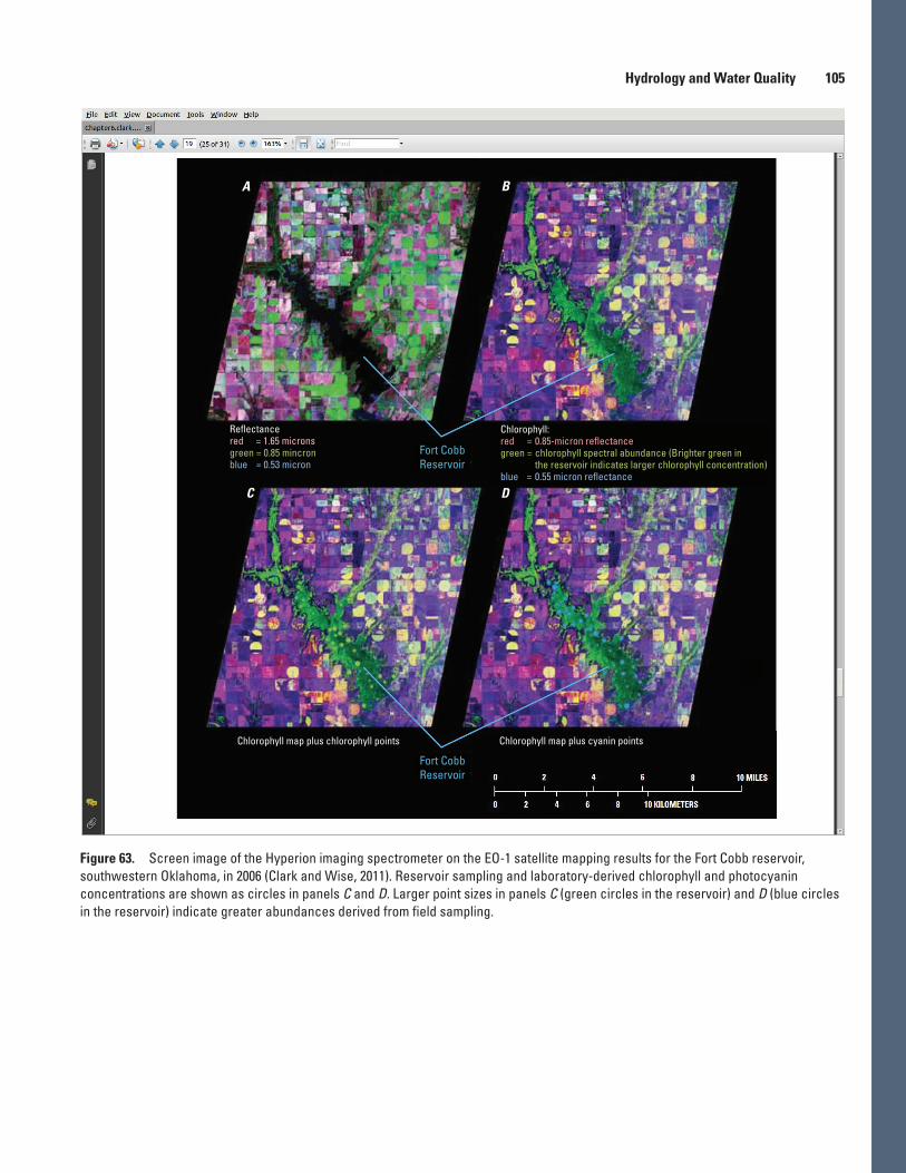
Hydrology and Water Quality 105
Figure 63. Screen image of the Hyperion imaging spectrometer on the EO-1 satellite mapping results for the Fort Cobb reservoir, southwestern Oklahoma, in 2006 (Clark and Wise, 2011). Reservoir sampling and laboratory-derived chlorophyll and photocyanin concentrations are shown as circles in panels C and D. Larger point sizes in panels C (green circles in the reservoir) and D (blue circles in the reservoir) indicate greater abundances derived from field sampling.
A B
C D
Reflectancered = 1.65 micronsgreen = 0.85 mincronblue = 0.53 micron
:
Chlorophyll:red = 0.85-micron reflectancegreen = chlorophyll spectral abundance (Brighter green in the reservoir indicates larger chlorophyll concentration)blue = 0.55 micron reflectance
Fort CobbReservoir
Fort CobbReservoir
Chlorophyll map plus chlorophyll points Chlorophyll map plus cyanin points
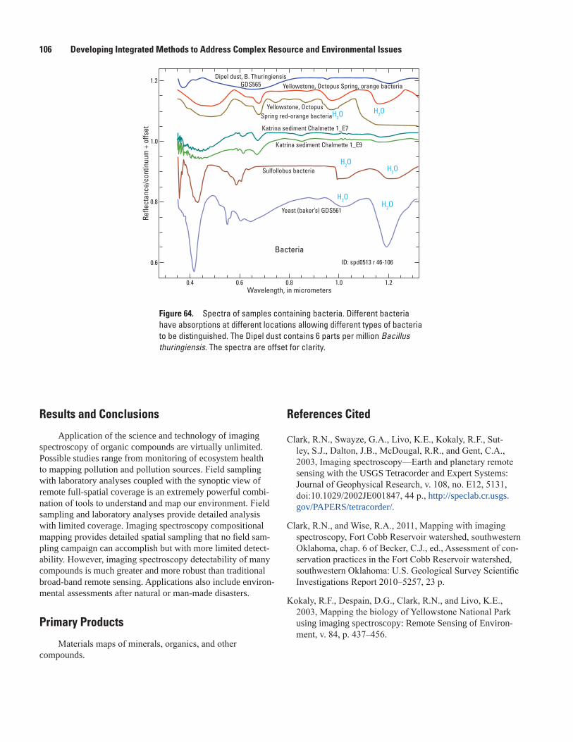
106 Developing Integrated Methods to Address Complex Resource and Environmental Issues
Refle
ctan
ce/c
ontin
uum
+ o
ffset
Wavelength, in micrometers
1.2
1.0
0.8
0.6
0.4 0.6 0.8 1.0 1.2
Bacteria
Yeast (baker’s) GDS561
ID: spd0513 r 46-106
Sulfollobus bacteria
Katrina sediment Chalmette 1_E9
Katrina sediment Chalmette 1_E7
H2OH2O
H2OH2O
H2OH2O
Yellowstone, Octopus Spring, orange bacteriaDipel dust, B. Thuringiensis
GDS565
Yellowstone, Octopus Spring red-orange bacteria
Figure 64. Spectra of samples containing bacteria. Different bacteria have absorptions at different locations allowing different types of bacteria to be distinguished. The Dipel dust contains 6 parts per million Bacillus thuringiensis. The spectra are offset for clarity.
Results and Conclusions
Application of the science and technology of imaging spectroscopy of organic compounds are virtually unlimited. Possible studies range from monitoring of ecosystem health to mapping pollution and pollution sources. Field sampling with laboratory analyses coupled with the synoptic view of remote full-spatial coverage is an extremely powerful combi-nation of tools to understand and map our environment. Field sampling and laboratory analyses provide detailed analysis with limited coverage. Imaging spectroscopy compositional mapping provides detailed spatial sampling that no field sam-pling campaign can accomplish but with more limited detect-ability. However, imaging spectroscopy detectability of many compounds is much greater and more robust than traditional broad-band remote sensing. Applications also include environ-mental assessments after natural or man-made disasters.
Primary Products
Materials maps of minerals, organics, and other compounds.
References Cited
Clark, R.N., Swayze, G.A., Livo, K.E., Kokaly, R.F., Sut-ley, S.J., Dalton, J.B., McDougal, R.R., and Gent, C.A., 2003, Imaging spectroscopy—Earth and planetary remote sensing with the USGS Tetracorder and Expert Systems: Journal of Geophysical Research, v. 108, no. E12, 5131, doi:10.1029/2002JE001847, 44 p., http://speclab.cr.usgs.gov/PAPERS/tetracorder/.
Clark, R.N., and Wise, R.A., 2011, Mapping with imaging spectroscopy, Fort Cobb Reservoir watershed, southwestern Oklahoma, chap. 6 of Becker, C.J., ed., Assessment of con-servation practices in the Fort Cobb Reservoir watershed, southwestern Oklahoma: U.S. Geological Survey Scientific Investigations Report 2010–5257, 23 p.
Kokaly, R.F., Despain, D.G., Clark, R.N., and Livo, K.E., 2003, Mapping the biology of Yellowstone National Park using imaging spectroscopy: Remote Sensing of Environ-ment, v. 84, p. 437–456.

Hydrology and Water Quality 107
Figure 65. Tetracorder (Clark and others, 2003) materials maps for Norris Geyser Basin in Yellowstone National Park using data from the NASA Airborne Visible and Infrared Imaging Spectrometer (AVIRIS). Minerals and bacteria are detected and mapped with the same data set. RGB, red, green and blue light added together.
Mineral map
RGB composite
Hot Springs biota
Hot Springs bacteria−Synochoccus
Mudflat
Algae−Cyanidium
Hot Springs bacteria
Hot Springs bacteria
Chalcedony
Halloysite
Alunite (50%) + Kaolinite (50%)
Montmorillonite−Calcium
Kaolinite−Well crystalline
Kaolinite−Poorly crystalline
EXPLANATION
EXPLANATION

108 Developing Integrated Methods to Address Complex Resource and Environmental Issues
Aeromagnetic Methods for Mapping Covered Faults in Sediments
By V.J.S. Grauch
Issue and Scope
The Rio Grande rift in New Mexico and Colorado is a series of linked sedimentary basins that formed during the past 25–30 million years through faulting and earthquake activity as the crust pulled apart. Sediments that filled the deepening basins now represent important aquifers supplying most of the drinking water for the cities of Albuquerque, Santa Fe, and Taos, New Mexico, as well as irrigation water for agricultural use in the San Luis Valley, Colorado. Normal faults bound the edges of the basins and are also numerous throughout the sedi-mentary section within the basins where many are concealed just below the ground. Although many of the faults are cur-rently inactive, their presence has an influence on groundwater flow through the aquifers, upward migration of hot water associated with geothermal energy resources, and transmission of seismic energy throughout the basin if an earthquake were to occur. Moreover, normal faults with large displacements can potentially form major boundaries between aquifers of very different hydraulic properties. Thus, accurately mapping faults within the basins and estimating fault displacements is important for improving models related to groundwater flow, geothermal resource potential, and seismic hazards.
During a previous study of the sedimentary basin sur-rounding the city of Albuquerque by the U.S. Geological Survey (USGS), unconventional application of aeromagnetic methods successfully detected signals from many intraba-sin faults (Grauch, 2001). At a regional scale, the magnetic expressions of the faults, called anomalies, were easy-to-follow linear features in aeromagnetic data images. At more local scales, however, the aeromagnetic expression was quite varied, both between faults and along the strike of individual faults. Some of the anomaly shapes appeared inconsistent with anomalies expected from simple normal faults. Standard methods to locate faults from aeromagnetic data proved to be inaccurate for these types of anomalies, so a better approach was required.
Objectives
This study involved the development of methods for mapping covered faults from aeromagnetic data acquired for sedimentary basins, with a focus on the anomalies with unexpected shapes. The objectives were to locate concealed fault traces as accurately as possible from gridded aeromag-netic data and to provide some insight on the amount of fault displacement from analysis of individual anomalies.
Background
The approach focused on modeling the range of sources of the fault anomalies using known faults as guides. As part of a related project, detailed geophysical and rock-property studies of exposed faults provided evidence that the aero-magnetic anomalies are produced by the juxtaposition of magnetically differing strata as opposed to chemical pro-cesses acting at the fault zone (Grauch and Hudson, 2007; Hudson and others, 2008). From these results, hypothetical models of juxtaposed strata were developed to represent the whole range of possible types of fault anomalies. The hypo-thetical models were then used to test methods of mapping fault traces and strategies for approximating fault throw from known or estimated geophysical parameters.
Results and Conclusions
The wide variety of anomaly shapes possible from juxtaposed strata can be characterized by four simple end-member hypothetical geophysical models, two of which fit traditional fault models and two of which do not (Grauch and Hudson, 2011). In map view, computing derivatives of gridded data (such as the horizontal gradient magnitude of the reduced-to-pole data) can help interpreters distinguish nontraditional fault-related anomalies from other geologic interpretations. Faults that are represented by the two non-traditional models produce parallel, double-track ridges in the horizontal derivative map, as demonstrated in figure 66. One of the parallel ridges is characteristically narrower than the other, which identifies the source as juxtaposed strata as opposed to other types of linear geologic sources, such as paleochannels or fault-zone alteration. Based on the model analysis, the trace of the fault is located most accurately by following the narrower of the two ridges. Thus, interpreters are able to map fault traces from the aeromagnetic data even where the anomaly shapes are unusual.
An examination of the relations between the geophysi-cal parameters for the simplest of the four end-member models of juxtaposed strata allows us to estimate the criteria required to produce detectable aeromagnetic anomalies for a given survey design. The relations between fault throw, magnetic properties, and depth of the fault are presented in graphical form for ease of use (Grauch and Hudson, 2007, 2011), which allows an interpreter to estimate fault throw from observed aeromagnetic data. In addition, the graphs are useful for planning new aeromagnetic surveys over sedimen-tary basins, assessing the amount of fault throw required to produce an aeromagnetic anomaly in a particular area, and estimating the depths to which these faults will be detected. These methods can also be applied to areas of layered geol-ogy outside the sedimentary environment, such as fields of layered volcanic flows.
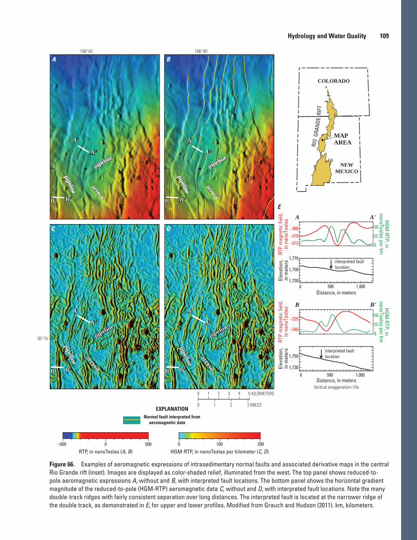
Hydrology and Water Quality 109
Figure 66. Examples of aeromagnetic expressions of intrasedimentary normal faults and associated derivative maps in the central Rio Grande rift (inset). Images are displayed as color-shaded relief, illuminated from the west. The top panel shows reduced-to-pole aeromagnetic expressions A, without and B, with interpreted fault locations. The bottom panel shows the horizontal gradient magnitude of the reduced-to-pole (HGM-RTP) aeromagnetic data C, without and D, with interpreted fault locations. Note the many double-track ridges with fairly consistent separation over long distances. The interpreted fault is located at the narrower ridge of the double track, as demonstrated in E, for upper and lower profiles. Modified from Grauch and Hudson (2011). km, kilometers.
pipelinepipelin
earroyo
pipeline
arroyo
A
A'
B B'
A
A'
B B'
0 100 200
HGM-RTP, in nanoTeslas per kilometer (C, D)
D
B B'
–340
–335
RTP
mag
netic
fiel
d,in
nan
oTes
las
25
50
0
HGM-RTP, in
nanoTeslas per km
Distance, in meters500 1,000
1,750
1,730Elev
atio
n,in
met
ers
0
Vertical exaggeration=10x
interpreted faultlocation
C
E
1,0001,730
1,750
1,770
0 500
interpreted faultlocation
Distance, in meters
Elev
atio
n,in
met
ers
A A'
–372–370
–368
25
50
0
HGM-RTP, in
nanoTeslas per km
RTP
mag
netic
fiel
d,in
nan
oTes
las
–500 0 500
RTP, in nanoTeslas (A, B)
EXPLANATION
pipelinepipelin
earroyo
pipelinepipelin
earroyo
pipeline
pipeline
arroyo
pipeline
pipeline
arroyo
pipeline
pipeline
arroyo
pipeline
pipeline
arroyo
pipeline
pipeline
arroyo
pipeline
pipeline
arroyo
pipeline
pipeline
arroyo
pipeline
pipeline
arroyo
106°45'106°45'
35°15'
5 KILOMETERS1 2 3 40
0 1 2 3 MILES
A
A'
B B'
A
A'
B B'
NM
MAPAREARI
O G
RAN
DE R
IFT
COLORADO
NEWMEXICO
A B
Normal fault interpreted from aeromagnetic data

110 Developing Integrated Methods to Address Complex Resource and Environmental Issues
Related U.S. Geological Survey Project
Geologic Framework of Rio Grande Basins Project, funded by National Cooperative Geologic Mapping and Min-eral Resources Programs.
References Cited
Grauch, V.J.S., 2001, High-resolution aeromagnetic data, a new tool for mapping intrabasinal faults—Example from the Albuquerque Basin, New Mexico: Geology, v. 29, no. 4, p. 367–370.
Grauch, V.J.S., and Hudson, M.R., 2007, Guides to under-standing the aeromagnetic expression of faults in sedimen-tary basins—Lessons learned from the central Rio Grande rift, New Mexico: Geosphere, v. 3, no. 6, p. 596–623, DOI: 10.1130/GES00128.1.
Grauch, V.J.S., and Hudson, M.R., 2011, Aeromagnetic anomalies over faulted strata: The Leading Edge, v. 30, no. 11, p. 1242–1252.
Hudson, M.R., Grauch, V.J.S., and Minor, S.A., 2008, Rock magnetic characterization of faulted sediments with associ-ated magnetic anomalies in the Albuquerque Basin, Rio Grande rift, New Mexico: Geological Society of America Bulletin, v. 120, no. 5/6, p. 641–658.
Constraints on Rio Grande Rift Structure and Stratigraphy from 3-D Magnetotelluric Modelling, Española Basin, New Mexico
By Brian D. Rodriguez and David A. Sawyer
Issue and Scope
The population of the Santa Fe region in northern New Mexico is growing. Water shortfalls in this low rainfall region could have serious consequences. Decisions for future growth and land management in the region depend on an accu-rate assessment and protection of the region’s groundwater resources. An important aspect of managing the groundwater resources is a better understanding of the hydrogeology of the Santa Fe Group and the nature of the sedimentary deposits that fill the Rio Grande rift, which contain the principal ground-water aquifers. The Santa Fe Group aquifer in the Española Basin is the main source of municipal water for the region.
Objectives
In collaboration with Black Oil, Inc., Los Alamos National Laboratories, New Mexico Bureau of Geology and Mineral Resources, and the U.S. Geological Survey (USGS) National Cooperative Geologic Mapping Program, project scientists used deep electrical geophysical measurements to provide con-straints for mapping subsurface stratigraphy and structure on the Rio Grande rift in the Española Basin. An improved under-standing of the geologic framework of the Española Basin in New Mexico (fig. 67) will provide more accurate hydrogeo-logic parameters for a newer generation of hydrologic models. This will ultimately better quantify estimates of future water supplies for northern New Mexico’s growing urban centers, which largely subsist on aquifers, primarily in the upper Santa Fe Group sediments, in basins of the Rio Grande rift.
Background
Electrical geophysical methods, and in particular the magnetotelluric (MT) method, have been used previously in mapping the subsurface structure within the Rio Grande rift and the deep crust. The MT method is capable of distinguish-ing rocks that are strong electrical conductors (such as thick clay-rich Mesozoic shales) from rocks that are moderately (for example, sandstones) or highly (for example, Cenozoic volcanic rocks or Precambrian crystalline rocks) electrically resistive. MT can also map electrically conductive rocks from shallow (about 100 meters) to very great (to greater than 10 kilometers) depths, provided they are thick enough and have a large enough electrical resistivity contrast with nearby rocks.

Hydrology and Water Quality 111
Figure 67. Simplified geologic map and cross section location of Santa Fe region, New Mexico, showing regional boreholes (solid red circles), magnetotelluric (MT) stations (green circles), and the MT profile cross section (solid black line). Colored polygons (modified from Green and Jones, 1997) represent major exposed geologic targets that are mapped in the subsurface using MT sounding.
27
1 3
35A'
Cerros del Riovolcanic field
Santa Fe
Los Alamos
Española
VALLES CALDERA
36°00'
106°30' 106°00'
ASanto Domingo
basin
I-25
CERRILLOS UPLIFT
Españolabasin
I-25
U.S.
285
U.S. 285
35°30'
0 20 KILOMETERS10
0 5 10 MILES
Magnetotelluric stationWell
Precambrian crystalline rocks
Paleozoic sedimentary rocks
Mesozoic sedimentary rocks
Cenozoic Sante Fe Group
Cenozoic volcanic rocks
EXPLANATIONGeologic map units
NEW MEXICO
Maparea
2
34
14
28
15
3332
12
31
3036
17
11 5
2510
23 22
9
29
420
821

112 Developing Integrated Methods to Address Complex Resource and Environmental Issues
Borehole data from 45 exploratory wells that penetrate the Rio Grande rift or the related sedimentary rocks drilled on the flanks of the rift are used to calibrate our models of the electrical properties of lithologic units known or predicted to underlie the rift. This is particularly important where there is a thick electrically conductive unit (for example, Meso-zoic shales) that underlay more resistive volcanic rocks (for example, Cenozoic basalts).
Results and Conclusions
Based on borehole resistivity data, Santa Fe Group sedi-ments are conductive to moderately resistive (4–44 ohm-m) on average, whereas Cenozoic igneous rocks are resistive (greater than about 200 ohm-m). Resistivity data for the Mesozoic shales indicate that they are strong electrical conductors (about 4–8 ohm meters [ohm-m]). Where the shales occur in the upper kilometer of crust, they may function as local hydrogeo-logic basement (separating older saline basinal waters from younger fresher groundwater). Paleozoic rocks generally have both moderately conductive and moderately resistive signa-tures (about 11–33 ohm-m). Precambrian crystalline rocks are resistive (greater than 600 ohm-m on average).
MT measurements provide additional constraints on the relative positions of basement rocks and the thicknesses of Paleozoic, Mesozoic, and Cenozoic sedimentary rocks in the Española Basin. The northern extent of a basement high (Cerrillos uplift, fig. 68) beneath the Cerros del Rio volcanic field (fig. 67) is delineated. The resistivity model also helps constrain models of the thickness of the upper Santa Fe Group (the coarser grained facies of Santa Fe Group sediments and primary aquifer in the region).
By correlating our resistivity model with surface geology and the deeper stratigraphic horizons using the deep well log data, we are able to interpret with more confidence which of the resistivity variations in the upper 2 kilometers belong to the upper Santa Fe Group sediments. The MT data primarily constrain the composite thickness of the conductive Cenozoic, Mesozoic, and upper Paleozoic sedimentary rocks that overlie more resistive lower Paleozoic sedimentary rocks and Precambrian basement.
Collaborators
Black Oil, Inc. Los Alamos National Laboratories New Mexico Bureau of Geology and Mineral Resources USGS National Cooperative Geologic Mapping Program
Selected References
Grauch, V.J.S., Phillips, J.D., Koning, D.J., Johnson, P.S., and Bankey, Viki, 2009, Geophysical interpretations of the southern Española Basin, New Mexico, that contribute to understanding its hydrogeologic framework: U.S. Geologi-cal Survey Professional Paper 1761, 88 p.
Green, G.N., and Jones, G.E., 1997, The digital geologic map of New Mexico in ARC/INFO format: U.S. Geological Survey Open-File Report 97–0052, 9 p., at https://pubs.er.usgs.gov/publication/ofr9752.
Figure 68. Profile A–A′ is a resistivity section extracted from the 3-D resistivity model with gross lithologic interpretation. Numbered labels at the top of the model are MT station numbers. Numbers in parentheses within the section are modeled resistivity in ohm-meters. The thick dashed line is the basin-floor model from Grauch and others (2009). The thin dashed line is the interpreted top of Precambrian (poorly constrained by MT data).
|04
|
20 |08
|
21 |11
|
05 |25
|
10 |23
|
22 |09
|
270
Volcanic rocks of the Cerros del Rio Volcanic Field(24-1000 ohm-meters)
A A'NORTHSOUTH
DEPTH, INMETERS
3,000
2,000
5,000
upper Santa Fe Group
lower Santa Fe Group(?)
Mesozoic(?)Paleozoic(?)
Precambrian(?)
CERRILLOS UPLIFT(6 ohm-meters)
(6–24 ohm-meters)
(33–44 ohm-meters)
(100–1,000 ohm-meters)
4,000
1,000
NO VERTICAL EXAGGERATION0 4,000 METERS2,000
0 4,000 8,000 FEET

Hydrology and Water Quality 113
Hudson, M.R., Grauch, V.J.S., Pantea, M.P., Koning, D.J., Johnson, P.S., Rodriguez, B.D., Minor, S.A., Caine, J.S., and Sawyer, D.S., 2009, Updated 3D model of the geologi-cal and geophysical framework of the southern Espanola Basin near Santa Fe, New Mexico, in Simmons, A., ed., Geology and hydrology of the Española Basin: Proceedings of the 7th Annual Española Basin Workshop, Santa Fe, New Mexico, March 6, 2008, New Mexico Bureau of Geology and Mineral Resources Open-File Report 513, p. 10.
Koning, D.J., Grauch, V.J.S., and Rodriguez, B.D., 2010, Cross-sections and geologic map for the eastern Española Basin, Rio Grande rift, north-central New Mexico, in Sim-mons, A., ed., The link between science and water policy: Proceedings of the 8th Annual Española Basin Workshop, Santa Fe, New Mexico, March 3, 2009, New Mexico Bureau of Geology and Mineral Resources Open-File Report 525, p. 11.
Rodriguez, B.D., and Sawyer, D.A, 2007, Correlation of magnetotelluric resistivity soundings and regional borehole geophysical rock properties to stratigraphy of the northern Rio Grande rift, New Mexico [abs.]: Geological Society of America Abstracts with Programs, v. 39, no. 6, p. 494.
Rodriguez, B.D., and Sawyer, D.A., 2008, Magnetotelluric soundings and deep borehole geophysical data constrain interpretations of subsurface geology of the southern Espa-ñola Basin, New Mexico, in Borchert, C.I., ed., Geologic and hydrogeologic framework of the Española Basin: Pro-ceedings of the 6th Annual Española Basin Workshop, Santa Fe, New Mexico, March 6, 2007, New Mexico Bureau of Geology and Mineral Resources Open-File Report 508, p. 7.
Rodriguez, B.D., and Sawyer, D.A., 2009, Geophysical con-straints of Rio Grande rift structure and stratigraphy based on magnetotelluric resistivity soundings and regional bore-hole geophysical rock properties, Northern New Mexico, in Simmons, A., ed., Geology and hydrology of the Española Basin: Proceedings of the 7th Annual Española Basin Work-shop, Santa Fe, New Mexico, March 6, 2008, New Mexico Bureau of Geology and Mineral Resources, Open-File Report 513, p. 18
Rodriguez, B.D., and Sawyer, D.A., 2013, Geophysical constraints on Rio Grande rift structure and stratigraphy from magnetotelluric models and borehole resistivity logs, northern New Mexico, in Hudson, M.R., and Grauch, V.J.S., eds., New Perspectives on Rio Grande Rift Basins: From Tectonics to Groundwater: Geological Society of America Special Paper 494, p. 323–344, doi:10.1130/2013.2494(13).
Providing a Subsurface Framework for Regional Groundwater Models of Alluvial Basins—Example from the Southern Española Basin, North-Central New Mexico
By V.J.S. Grauch and Jeffrey D. Phillips
Issue and Scope
Alluvial basins that follow the Rio Grande in north-central and northern New Mexico contain sediments that are important aquifers for communities such as Albuquerque, Santa Fe, Española, Taos, eight Pueblo nations, and surround-ing suburban areas. Regional groundwater-flow models are commonly constructed to help manage and regulate these groundwater resources. Thus, accurate models are important but are hindered by lack of information in between scattered water wells. In particular, estimating the thickness of the basin-fill sediments is important for estimating the maximum storage capacity of the aquifer.
Traditionally, aeromagnetic methods have been under-utilized for determining the thickness of basin-fill sediments, yet the geology in many areas of the alluvial basins along the Rio Grande is favorable for this approach. A good example is in the southern Española Basin, south of the city of Santa Fe, New Mexico. In this area, weakly magnetic sediments, which make up the alluvial aquifer, are locally underlain by older, moderately to strongly magnetic igneous and volca-niclastic rocks. Because aeromagnetic data (measurements of the magnetic field from aircraft) are most sensitive to the underlying moderately to strongly magnetic rocks, estimating the depths to the tops of the igneous and volcaniclastic rocks also indicates the thickness of overlying sediments. Thus, the maximum thickness of the aquifer can be estimated from quantitative analysis of high-resolution aeromagnetic data acquired over the region.
Objectives
Many methods for estimating depth to magnetic sources from aeromagnetic data have been developed previously. The methods generally provide the depth to the shallowest, most magnetic source. Because no one method is the best for all situations and amount of noise in the data (Phillips, 2000), the best approach to using magnetic depth estimation is to investi-gate the results of multiple methods.
Although the situation for the southern Española Basin appeared ideal for using magnetic depth-estimation methods to map the base of the aquifer, preliminary results (Phillips and Grauch, 2004) revealed some important difficulties. The difficulties arose because the shallowest, most magnetic source

114
Developing Integrated Methods to Address Com
plex Resource and Environmental Issues
–1,000
0
1,000
2,000
Elev
atio
n, in
met
ers
3,980,000 3,970,000 3,960,000 3,950,0003,990,000 3,940,000 3,930,000 3,920,000
Northing, in meters VERTICAL EXAGGERATION = 4X
–1,500
–1,000
–500
0
500
1,000
1,500
2,000
2,500
Elevation, in meters
Cerrillos Hills
SantaFe
Cerrillos Hills
SantaFe
SANTA FE MOUNTAINS
SANTA FE MOUNTAINS
Española
Española25
84
68
285
285
NEWMEXICO
COLORADO
TEXAS
R
IO
G
RAN
DE
RI
FT
RioGrande
Santa FeAlbuquerque
Taos
Alamosa
Socorro
MEXICO
EXPLANATION
N
Figure 69. Perspective view of the modeled elevation of the base of the alluvial aquifer in the southern Española Basin in relation to topography, looking east. Topographic surface is raised above the base. From Grauch and others (2009).

Hydrology and Water Quality 115
was generally, but not always, located along the top of the igne-ous and volcaniclastic unit. In some cases, the sediments were magnetic enough that they represented the shallowest, magnetic source. In other cases, variability in layers of the underlying igneous and volcanic unit produced magnetic layers internal to the unit that were more magnetic than its top. Thus, the objec-tives of this study were to (1) apply a variety of depth-estimation methods developed under the auspices of the Integrated Methods Development Project to the southern Española Basin, and (2) combine the depth-estimate results with information from other geologic and geophysical data in a 3-D environment to obtain a consistent surface representing the base of the aquifer.
Background
Magnetic depth-estimation methods examined or devel-oped under the auspices of the Integrated Methods Development Project were applied to aeromagnetic data from the southern Española Basin in profile and gridded form separately. Profiles were analyzed by using the computer program PDEPTH (Phil-lips, 1997), which incorporates a variety of methods so that results can be examined together. Gridded data were analyzed using adaptations of the local wave-number method (Thurston and Smith, 1997; Smith and others, 1998; Phillips and others, 2007) and two-step extended Euler method (Reid and others, 1990; Nabighian and Hansen, 2001; Phillips, 2002; Phillips and Grauch, 2004). The results of depth estimation were then incorporated into a 3-D model developed by Grauch and others (2009) using the software package GeoModeller.™
Results and Conclusions
The depth-estimate solutions from profile versus grid-ded data were brought into the 3-D model in different ways. Depth-estimate solutions for profile data were used to develop 2-D geophysical models along the same profiles. The 2-D models were then incorporated directly into the 3-D model, rather than the depth-estimate solutions themselves. In con-trast, the 3-D locations of more than 100,000 depth-estimate solutions from the grid-based methods were input directly into the 3-D model. This direct input allowed us to project the solu-tion locations onto any desired 2-D section for inspection in relation to other geologic and geophysical information.
Comparison of gridded depth-estimate solutions in the 3-D modeling environment with other geophysical informa-tion and well data proved invaluable for resolving difficulties presented by variable magnetic sources. Using this approach, depth estimates locating the top of the igneous and volcani-clastic unit could easily be distinguished from those locating other magnetic interfaces internal to this unit or within the sediments above it. Finally, combining the improved under-standing of the magnetic depth-estimate solutions with other geophysical information and well data allowed us to develop a 3-D model of the base of the aquifer for the southern Española Basin (fig. 69; Grauch and others, 2009).
Related U.S. Geological Survey Project
Geologic Framework of Rio Grande Basins Project, funded by National Cooperative Geologic Mapping and Mineral Resources Programs
References Cited
Grauch, V.J.S., Phillips, J.D., Koning, D.J., Johnson, P.S., and Bankey, Viki, 2009, Geophysical interpretations of the southern Española Basin, New Mexico, that contribute to understanding its hydrogeologic framework: U.S. Geologi-cal Survey Professional Paper 1761, 88 p., at http://pubs.usgs.gov/pp/1761/.
Nabighian, M.N., and Hansen, R.O., 2001, Unification of Euler and Werner deconvolution in three dimensions via the generalized Hilbert transform: Geophysics, v. 66, p. 1805–1810.
Phillips, J.D., 1997, Potential-field geophysical software for the PC, version 2.2: U.S. Geological Survey Open-File Report 97–725; unpaged, at http://pubs.usgs.gov/of/1997/ofr-97-0725/.
Phillips, J.D, 2000, Locating magnetic contacts—A compari-son of the horizontal gradient, analytic signal, and local wavenumber methods [abs.]: Annual International Meeting of Society of Exploration Geophysicists, 70th, Expanded Abstracts, v. 19, p. 402–405, at http://seg.org/publications/archive/exAbsHist/abs_pdf/2000/ea200004020405.pdf.
Phillips, J.D., 2002, Two-step processing for 3D magnetic source locations and structural indices using extended Euler or analytic signal methods [abs.]: Society of Explo-ration Geophysicists, 2002 Technical Program Expanded Abstracts, 4 p.
Phillips, J.D., and Grauch, V.J.S., 2004, Thickness of Santa Fe Group sediments in the Española Basin south of Santa Fe, New Mexico, as estimated from aeromagnetic data: U.S. Geological Survey Open-File Report 2004–1354, 24 p., at http://pubs.usgs.gov/of/2004/1354/.
Phillips, J.D., Hansen, R.O., and Blakely, R.J., 2007, The use of curvature in potential-field interpretation: Exploration Geophysics, v. 38, p. 111–119.
Reid, A.B., Allsop, J.M., Granser, H., Millett, A.J., and Somer-ton, I.W., 1990, Magnetic interpretation in three dimensions using Euler deconvolution: Geophysics, v. 55, p. 80–91.
Smith, R.S., Thurston, J.B., Dai, Ting-Fan, and MacLeod, I.N., 1998, iSPITM—The improved source parameter imaging method: Geophysical Prospecting, v. 46, p. 141–151.
Thurston, J.B., and Smith, R.S., 1997, Automatic conversion of magnetic data to depth, dip, and susceptibility contrast using the SPITM method: Geophysics, v. 62, p. 807–813.

Hazards and Disaster Assessment
significantly reducing the magnetization of volcanic rocks. These changes in rock properties produce clear distinctions between altered and unaltered rock in geophysical survey measurements. The presence of water helps form clay miner-als that weaken the edifice but also reduce pore pressures, increasing the potential for slope failure. In addition, water and entrained melting ice acts as a lubricant to transform debris avalanches into lahars.
The objectives of this study are to determine the 3-D distribution of alteration and water on Mount Rainier, Mount Baker, and Mount Adams with HEM data to aid in hazards, water-resource, and mineral studies. The rugged, magnetic, and resistive volcanoes pose difficulties in data collection and analysis. We applied a variety of data reduction and model-ing approaches to obtain 3-D models of the composition of the volcanoes. In order to tie the results of the modeling to the geology, we measured electrical and magnetic properties of representative samples from each volcano.
Background
Analysis and modeling of the magnetic and HEM data required application of techniques developed at the U.S. Geo-logical Survey (USGS) including filtering, depth estimates, equivalent source determination, and magnetic (Phillips, 1992, 1997, 2000, 2001, 2007) and HEM modeling. The results from application of these techniques helped constrain modeling of the magnetic and electromagnetic data. In addition, electrical resistivity, susceptibility, and density of rock samples were measured in the USGS Petrophysics laboratory to help con-strain the 3-D geophysical models. Samples ranged from fresh, massive andesite and dacite to completely altered powders composed of opal, alunite, kaolinite, and montmorillonite.
Results and Conclusions
Combined HEM and magnetic models (fig. 70) show that appreciable thickness (>500 meters [m]) of low to moderate resistivity (0.1–100 ohm-meters), nonmagnetic, water-satu-rated hydrothermally altered material lies under ice west of the modern summit of Mount Rainier in the Sunset Amphi-theater region (Finn and others, 2001) and in the central core of Mount Adams north of the summit (Finn, Deszcz-Pan, and others, 2007) (dark blue zones in fig. 70). Alteration at Mount Baker is restricted to thinner (<300 m) zones beneath Sherman Crater and the Dorr Fumarole Field (Finn and Deszcz-Pan, 2009). These altered water-saturated rocks lie at shallow depths (1–90 m) beneath the ice. The magnetic model tends to show minimum thickness and cannot unequivocally determine the base of alteration, because of uncertainties and variability of magnetization contrasts.
Geophysics of Volcanic Landslide Hazards—Inside Story
By Carol A. Finn and Maria Deszcz-Pan
Issue and Scope
Hydrothermally altered rocks, particularly if water saturated, can weaken stratovolcanoes, thereby increasing the potential for catastrophic sector collapses that can lead to far-traveled, destructive debris flows or volcanic landslides. Evaluating the hazards associated with such alteration is dif-ficult because alteration has been mapped on few active volca-noes, and the distribution and severity of subsurface alteration is largely unknown on any active volcano. Large landslides from Mounts Adams, Baker, and Rainier are their primary hazards, not eruptions. Collapses of water-saturated hydrother-mally altered edifice flanks from these volcanoes have gener-ated numerous extensive landslides, and future collapses could threaten areas that are now densely populated.
Traditional methods for evaluation of landslide hazards have been largely restricted to surficial mapping of volcanoes and landslide deposits. However, the applications of technolo-gies, rock property measurements, and analysis tools from the minerals industry can help delineate water-saturated and hydrothermally altered rock, thereby aiding in volcanic land-slide hazards assessments.
Objectives
Critical to quantifying the hazard from volcanic land-slides is knowledge of the three-dimensional (3-D) distribu-tion of pervasively altered rock and shallow groundwater that plays an important role in transforming debris avalanches to far-traveled lahars, which are the debris that flows down the slopes of a volcano (Vallance and Scott, 1997; Vallance, 1999), both of which can be detected by helicopter electro-magnetic (HEM) and magnetic data (Deszcz-Pan and others, 1998; Finn and others, 2001; Finn, Descsz-Pan, and others, 2007; Finn, Deszcz-Pan, Anderson, and John, 2007; Finn and Deszcz-Pan, 2009; Finn and Descsz-Pan, 2011). Hydrother-mally altered volcanic rocks possess low electrical resistivi-ties because of their water and clay contents, whereas high resistivities characterize fresh, dry, massive volcanic rocks. Low to moderate resistivities characterize groundwater of various salinities (Keller, 1987; Finizola and others, 2006). Magnetic data reflect variations in the distribution and type of magnetic minerals, primarily magnetite, in the Earth’s crust. Hydrothermal alteration generally destroys magnetite,

Hazards and Disaster Assessment 117
Figure 70. Three-dimensional view of the distribution of water and alteration based on geologic mapping, resistivity (upper 300 meters), and magnetic (>300-meter thickness) models and measured rock properties.
Dry, fresh rock or ice Saturated, intensely altered rock
Saturated, fresh or weakly altered rock
Moist intensely altered rock
Intensely altered rock (saturation level unknown)
EXPLANATION
A Mount Adams
Resistivitymodel
Magneticmodel
WhiteSalmonGlacier
Summit
0
1,500
4,500
3,000
0
1,500
3,000
1,000
2,000
3,000
Elev
atio
n, in
met
ers
3,200
1,200
2,000
2,800
2,400
1,600Elev
atio
n, in
met
ers
0
2,000
4,000 4,000
2,000
0
4,000
1,000
2,000
3,000
Elev
atio
n, in
met
ers
SunsetAphitheater
Summit
Summit
Shermancrater
B Mount Baker
C Mount Rainier
Distance, in meters
Distance, in meters
N

118 Developing Integrated Methods to Address Complex Resource and Environmental Issues
Resistivities of 100–850 ohm-m characterize water-saturated fresh volcanic rocks (green in fig. 70). Given observed stratigraphy, the water is contained in permeable breccia bounded by impermeable lava flows. It is likely that water-rich rock lies below the 100–200 m detection depth of the HEM data. The magnetic data identify low susceptibilities that likely represent intensely altered rock to depths of at least 1,000 m below the surface; water could occupy pore space in these rocks as they do near the surface. Several geologic observations support the geophysical identification of water-rich layers: alteration is strongly controlled by permeability and the presence of water; the presence of opal and other silica phases near the summit that form at and below the water table; and reconnaissance stable isotope data of hydrothermal miner-als that indicate formation predominantly from groundwater (John and others, 2008). These permeable units most likely represent local perched water units. The HEM data identified water-saturated rocks from the surface to the detection limit (100–200 m) in discreet zones at Mount Rainier (Finn and others, 2001) and Mount Adams (Finn, Deszcz-Pan, Anderson, and John, 2007) and over the entire summit region at Mount Baker (Finn and Deszcz-Pan, 2009).
Ice thickness measurements critical for flood and landslide hazards studies are very sparse on Cascade Range volcanoes. The HEM data were used to determine ice thick-ness over portions of Mount Baker and Mount Adams volca-noes. A variety of HEM modeling techniques were applied to the data. Resistivity sections provide good estimates of ice thickness where the basement is altered and conductive. In general, ice thicknesses less than 100 m over low- to moderate-resistivity basement are well-resolved. Estimates greater than ≈100 m are not resolved nor were those over very high resistivity (>1,000 ohm-m) basement. The ice thicknesses derived from HEM are consistent with the previous drill-hole data from Mount Adams and radar data from both volcanoes with mean thickness of 31 m for Mount Adams and 43 m for Mount Baker. The resulting ice thick-ness maps show that the thickest ice on Mount Baker is on the gentle lower slopes and the thickest ice at Mount Adams is at the summit (Finn and others, 2012).
The application of helicopter magnetic and HEM meth-ods, traditional tools of the mining industry, to geotechnical studies of volcanoes is challenging due to high elevation and rugged, magnetic, and resistive terrain. Difficult flight condi-tions can result in uneven flight lines at less than optimum heights above the ground for modeling. Due to highly magnetic volcanic rocks, small changes in elevations over the sources, especially over deep valleys, make modeling difficult resulting in unrealistic geometries in some cases in the upper 100–200 m of the models. The high resistivities make differentiating between thick ice and rock and identifying water in fresh vol-canic rocks difficult. However, combining magnetic and HEM data with geology and rock property measurements and innova-tive modeling approaches allows identification of alteration and water and ice thickness critical to evaluating volcanic landslide hazards and water and ice availability to the landslides.
Collaborators
Thomas Sission, Mark Reid, David John, George Breit, and Robert Horton, all U.S. Geological Survey.
References Cited
Deszcz-Pan, Maria, Fitterman, D.V., and Labson, V.F., 1998, Reduction of inversion errors in helicopter EM data using auxiliary information: Exploration Geophysics, v. 29, p. 142–146.
Finizola, A., Revil, A., Rizzo, E., Piscitelli, S., Ricci, T., Morin, J., Angeletti, B., Mocochain, L., and Sortino, F., 2006, Hydrogeologic insights at Stromboli volcano (Italy) from geoelectrical, temperature, and CO2 soil degassing investigations: Geophysical Research Letters, v. 33, 4 p., doi:10.1029/2006GL026842.
Finn, C.A., and Deszcz-Pan, Maria, 2009, The 3-D distribution of alteration, ice and water from helicopter magnetic and electromagnetic surveys at Mts. Adams, Baker and Rainier, Washington—Implications for debris flows hazards [abs.]: Geological Society of America Abstracts with Programs, v. 41, p. 717.
Finn, C.A., and Descsz-Pan, Maria, 2011, Helicopter magnetic and electromagnetic surveys at Mounts Adams, Baker and Rainier, Washington—Implications for debris flow hazards and volcano hydrology [abs.]: International Workshop on Gravity, Electrical & Magnetic Methods and Their Applica-tions, Beijing, China, October 10–13, 2011: p. 24, http://dx.doi.org/10.1190/1.3659065.
Finn, C.A., Deszcz-Pan, Maryla, Anderson, E.D., and John, D.A., 2007, Three-dimensional geophysical mapping of rock alteration and water content at Mount Adams, Wash-ington—Implications for lahar hazards: Journal of Geo-physical Research, v. 112, 21 p.
Finn, C.A., Descsz-Pan, Maria, and Bedrosian, P.A., 2012, Helicopter electromagnetic data map ice thickness at Mount Adams and Mount Baker, Washington, USA: Journal of Glaciology, v. 58, no. 212, p. 1133–1143.
Finn, C.A., Deszcz-Pan, M., Horton, R., Breit, G., and John, D., 2007, Airborne magnetic and electromagnetic data map rock alteration and water content at Mount Adams, Mount Baker and Mount Rainier, Washington—Implications for lahar hazards and hydrothermal systems: Eos Transactions American Geophysical Union, v. 88, (Fall Meeting Supple-ment), Abstract NS34A-05.
Finn, C.A., Sisson, T.W., and Descsz-Pan, Maryla, 2001, Aerogeophysical measurements of collapse-prone hydro-thermally altered zones at Mount Rainier Volcano, Washing-ton: Nature, v. 409, p. 600–603.

Hazards and Disaster Assessment 119
John, D.A., Sisson, T.W., Breit, G.N., Rye, R.O., and Vallance, J.W., 2008, Characteristics, extent and origin of hydrother-mal alteration at Mount Rainier Volcano, Cascades arc, USA—Implications for debris-flow hazards and mineral deposits: Journal of Volcanology and Geothermal Research, v. 175, p. 289–314.
Keller, G.V., 1987, Rock and mineral properties: Investiga-tions in Geophysics, v. 3, p. 13–51.
Phillips, J.D., 1992, TERRACE: A terracing procedure for gridded data, with FORTRAN programs and VAX com-mand procedures, UNIX C-shell and DOS implimentations: U.S. Geological Survey Open-File Report 92–5, unpaged, at http://pubs.usgs.gov/of/1997/ofr-97-0725/.
Phillips, J.D., 1997, Potential-field geophysical software for the PC, version 2.2: U.S. Geological Survey Open-File Report 97–725, 34 p.
Phillips, J.D., 2000, Locating magnetic contacts—A com-parison of the horizontal gradient, analytic signal, and local wavenumber methods [abs.]: Society of Exploration Geophysicists Technical Program Expanded Abstracts, p. 402–405.
Phillips, J.D, 2001, Designing matched bandpass and azi-muthal filters for the separation of potential-field anomalies by source region and source type [abs]: Australian Society of Exploration Geophysicists, 15th Geophysical Conference and Exhibition, Expanded Abstracts, CD-ROM, p. 4.
Phillips, J.D., 2007, Geosoft eXecutables (GX’s) developed by the U.S. Geological Survey, version 2.0, with notes on GX development from Fortran code: U.S. Geological Survey Open-File Report 2007–1355, 111 p.
Vallance, J.W., 1999, Postglacial lahars and potential hazards in the White Salmon River system on the southwest flank of Mount Adams, Washington: U.S. Geological Survey Bul-letin 2161, 49 p.
Vallance, J.W., and Scott, K.M., 1997, The Osceola mudflow from Mount Rainier—Sedimentology and hazard implica-tions of a huge clay-rich debris flow: Geological Society of America Bulletin, v. 109, p. 143–163.
Helicopter Electromagnetic Surveys Over Volcanoes—Resolution and Limitations for Mapping Ice Thickness
By Maria Deszcz-Pan, Carol A. Finn, and Paul Bedrosian
Issue and Scope
The occurrence of floods and mudflows during the erup-tion of Mount St. Helens and documented large water-saturated mudflows from Mount Rainier and Mount Adams indicate the need for ice thickness measurements to help predict the water-hazard of Cascade volcanoes (Driedger and Kennard, 1986). The biggest hazards from Mount Baker and Mount Adams are not eruptions but debris avalanches and lahars partially lubri-cated by ice, snow, and melt water (Gardner, 1995; Scott and others, 1995; Vallance, 1999). Other hazards include removal of ice and snow during eruptions, which leads to flooding and melting of ice and snow that contributes to phreatic and hydro-thermal eruptions (Mastin, 1995). However, few ice thickness measurements have been directly made on these and other Cascade volcanoes (Driedger and Kennard, 1986).
Objectives
We report the pioneering use of helicopter electromagnetic (HEM) data, originally collected to detect hydrothermal altera-tion (Finn and others, 2001; Finn and others, 2007a,b; to estimate ice thickness for parts of Mount Baker and Mount Adams. We focus on the innovative approach of using resistivity inversions to obtain ice thickness and to quantify the limits and uncertain-ties in ice depth estimates. Comparisons of the HEM results with ice-penetrating radar measurements and drill-hole data help determine their reliability.
Background
To evaluate the reliability of determining ice thickness from the HEM data, we used a freeware program called EMMA (Auken and others, 2002) to provide expected ranges of ice thickness values for a specific HEM system and survey param-eters and for a resistivity model that approximates local geo-logic conditions. The resistivity model contains variably thick (0–125 meters [m]) resistive ice layer (10,000 ohm-m) over base-ment with variable resistivities. Figure 71 presents the results.
If the resistivity of the basement is low (for example, <100 ohm-m), the calculated ice thickness closely approxi-mates the true layer thickness for depths less than 60 m, is within about 10 m for ice thickness between 60 and ≈90 m, and errors may exceed 25 m for ice thickness >100 m (fig. 71). For 300 ohm-m basement resistivity, the uncertainty in ice thickness

120 Developing Integrated Methods to Address Complex Resource and Environmental Issues
Figure 72 (facing page). Example of cross section from Mount Adams two-layer laterally continuous inversions (Auken and others, 2005). A, Measured in-phase (I) component at five frequencies. B, Measured quadrature (Q) component at five frequencies. C, Inverted resistivity section with sensor elevation shown above topography. Sensor elevations are shown in red where they exceed 100 meters. Ice thickness, where reliable, is defined by the bottom of orange-brown ice layer. Gray lines indicate the upper and lower bounds on the ice thickness. Black line shows the depth of investigation. Vertical thin lines near summit indicate ice depths from the radar profile. D, Upper and lower bounds on the layer thickness. Lines are red where the solution is unreliable. E, Location of flight path from the top of Mount Adams volcano on aerial photograph. Borehole symbols are color-coded and show ice thickness from 1930s drill holes (Fowler, 1935); circles are also color-coded and show radar soundings over the summit ice cap (Tulaczyk, University of California, Santa Cruz, written commun., 2006).
Figure 71. Uncertainties in ice thickness estimates as a function of ice thickness and basement resistivity. The x-axis represents the true layer thickness and the y-axis represents the maximum and minimum thickness of ice estimated from the inversion of data at six frequencies, assuming a given noise (Auken and others, 2002) and 50-meter system elevation. Color-coded lines represent the expected range of thickness estimates depending on the basement resistivity compared to the true ice thickness shown in red. The curves are truncated where ice thickness resolution is low, chosen to be twice the true ice thickness value.
True ice thickness, in meters0 25 50 75 100 125
EXPLANATIONTrue layer thickness10 ohm-meter basement100 ohm-meter basement 850 ohm-meter basement
600 ohm-meter basement300 ohm-meter basement
0
25
50
75
100
125
Estim
ated
ice
thic
knes
s ra
nge,
in m
eter
s
estimate exceeds 25 m for 75-m-thick ice and is about 5 m for ice <≈50 m thick (fig. 71). For basement resistivities between 300 and ≈850 ohm-m, ice thickness <≈35 m can be deter-mined reliably. For thin ice (<≈10 m) and resistive basement (300–850 ohm-m), the ice thickness is not resolved, because there is not enough difference in response between them.
We invert the data for the ice thickness using one-dimensional (1-D) laterally constrained inversion (LCI) algo-rithm (Auken and others, 2005; Siemon, 2009). Because we are only interested in ice thickness, two layers are sufficient for the modeling, with the understanding that the uncertain-ties associated with the inverted top layer thickness provide a measure of uncertainties in ice thickness estimates. An example of one inverted line from the top of Mount Adams is given in figure 72C.
For LCI inversion we subdivided the profiles into blocks of ≈500 m with ≈50 soundings in each block, within which all 1-D datasets and models are inverted as one system, producing
layered sections with laterally smooth transitions within each block. Because the inversion consists only of two layers, a limited number of parameters need to be determined. For parameterized inversions, such as the two-layer inversion applied here, estimates of the standard deviation values for a given parameter (for example, layer thickness) were calculated directly from the model covariance matrix. The upper and lower limits of the inverted thickness of the top layer are plot-ted in figure 72D, where gray lines show well-resolved depths and red lines show unresolved or below the depth of investiga-tion (described in next paragraph) values.
An estimate of the maximum depth of reliable HEM inversion results, called the depth-of-investigation (DOI), is calculated by finely discretizing the final two-layer inverse model and calculating the sensitivity matrix for the redis-cretized model, resulting in a cumulative sum of column-wise averages of the sensitivity matrix (Christiansen and Auken, 2010). The DOI metric is subsequently defined as the depth at which data sensitivity drops below a threshold of 0.8. The black line on the cross section in figure 72C shows this boundary. This metric, one measure of DOI, is influenced by the regularization and starting model and is best used to assess relative lateral variations in the DOI rather than an absolute measure of DOI. Other gray lines on the cross section in figure 72C show the same upper and lower limits on layer thickness estimate as in figure 72D.
Results and Conclusions
The reliability of the ice thickness values depended on several factors. Figure 72 demonstrates that the signal levels (shown in figs. 72A and 72B for in-phase and quadrature com-ponents, respectively) are higher when the basement is conduc-tive (blue colors in fig. 72C), shallow, and when the measure-ment bird is closer to the Earth’s surface (compare line above

Hazards and Disaster Assessment 121
0
10
20
40
60
80
100
30
50
70
90
110 200
Ice thickness,in meters
1 5
45
80
140
215
300
370
450
520
600
675
750
850
950
1,000
5,500
10,000
20,000
615,000 616,000 617,000 618,000Easting, in meters
−500
0
500
Dist
ance
, in
met
ers
2,500
3,000
3,500
Elev
atio
n, in
met
ers
50
100
150
200
Thic
knes
s, in
met
ers
500
1,000
1,500
2,000
I, in
par
ts p
er m
illio
n
0
500
1,000
1,500
2,000
Q, in
par
ts p
er m
illio
n
614,000 619,000
100,000
25,000
6,200
3,300
1,500
400
E
D
C
B
A
Universal Transverse Mercator projection, zone 10 northNorth American Datum of 1927
Lower boundon ice thickness
Upper boundon ice thickness
Sensorelevation
Depth ofinvestigation
EXPLANATION
EXPLANATION
0 1,000 METERS
0 4,000 FEET
Resistivity,in ohm-meters
EXPLANATION
Signal frequency,in hertz

122 Developing Integrated Methods to Address Complex Resource and Environmental Issues
Seattle
MOUNT BAKER
MOUNT ADAMSMOUNT SAINT HELENS
MOUNT RAINIER
WASHINGTON
Map location
EXPLANATION
200 ohm-meter basement resistivity contour
Airborne electromagnetic flight path
−121°51' −121°49' −121°47'
drill hole and radarmeasurements
−121°31' −121°30' −121°29' −121°28'
Error, in meters
5045403530252015105
B
A
Universal Transverse Mercator projection, zone 10 northNorth American Datum of 1927
46°11'
46°12'
46°13'
48°46'
48°47'
Ice thickness, in meters
>110100 to 11090 to 10080 to 9070 to 8060 to 7050 to 6040 to 5030 to 4020 to 3010 to 20<10
CARMELOCRATER
SHERMANCRATER
EASTONGLACIER
WHITESALMON
KLICKITAT
LYMAN
WILSONADAMS
Figure 73. Ice thicknesses for Mounts Baker and Adams. A, Mount Baker ice thickness spot and gridded results overlain on aerial photographs based on helicopter electromagnetic (HEM) and radar data (squares) (Harper, 1993; Tucker and others, 2009; Park, 2011). Depths indicated by colors. Size is proportional to the absolute uncertainty in depth estimate expressed as a difference between gray lines in figure 72D. Black lines represent 200 ohm-meters basement resistivity contour. B, Mount Adams ice thickness spot and gridded results overlain on aerial photographs based on HEM, radar (Tulaczyk, University of California, Santa Cruz, written commun., 2006), and drill-hole (Fowler, 1935) data. Black lines represent 200 ohm-meters basement resistivity contour. Depths indicated by colors. Size is proportional to the absolute uncertainty in depth estimate expressed as a difference between gray lines in figure 72D.

Hazards and Disaster Assessment 123
inverted section in fig. 72C [showing the sensor elevation above the topography] with signal levels). The line is black when the elevation is less than 100 m and red for the sensor higher than 100 m. On Mount Adams, higher bird elevations and more resistive basement outside of the summit area produced lower signal levels (fig. 73B) yielding fewer ice thickness estimates than for Mount Baker (fig. 73A). The most reliable ice thickness values are located where the ice is <≈100 m thick over <200 ohm-m basement (figs. 73A and 73B). Over resistive basement (>≈200 ohm-m; contours figs. 73A and 73B), thicknesses are acceptable if the ice is <30–50 m thick but become increasingly unreliable with increasing resistivity and ice thickness (fig. 71) because of low signal levels and the limitations of the HEM method to differentiate between the resistive ice and rock layers (figs. 71, 72, and 73).
At Mount Baker, basement resistivities are generally <850 ohm-m, with large regions less than 200 ohm-m (contours, fig. 73A) (Finn and others, 2012) making ice thickness estimates possible over much of the survey area (fig. 73). Although ice thickness reaches about 75–80 m in Carmelo crater (fig. 73A), ice is generally thinner than ≈50 m, including Sherman Crater, at high elevations (fig. 73A). Ice thickness increases on the gentler slopes at the edge of the volcano to >100 m (fig. 73A). Radar measurements on Easton Glacier show that the ice maintains its >80-m thickness for nearly 2 kilometers south of the HEM survey region (Harper, 1993) suggesting that all glaciers could contain thick ice outside of the survey region (fig. 73A).
At Mount Adams, ice is thickest over the central and west-ern part of the summit ice cap, exceeding 120 m (fig. 73B). The upper reaches of the White Salmon, Adams, Lyman, and Klicki-tat Glaciers (fig. 73B) contain ice ranging in thickness from ≈25–60 m. The glaciers lower down on the volcano are less than ≈30 m thick. Inspection of the aerial photographs shows outcrop in many parts of the lower portions of the glaciers revealing thin ice (<10 m), especially in the south (fig. 73B). In general, thin ice mantles the steep slopes around Mount Adams where ice thickness increases with increasing elevation (fig. 73B).
The 1980 eruption of Mount St. Helens, the most active volcano in the Cascades, removed ≈130 x106 m3 of ice and snow, resulting in lahars and floods (Driedger and Kennard, 1986). Mount Baker is the second most-active volcano in the Cascades, with vigorous fumaroles in Sherman Crater, the site of thermal unrest in 1975 (Crider and others, 2011), where ice volumes are ≈1.3–2.1 x10⁶ m3 (Park, 2011). An eruption could result in significant melting of ice and snow into the water reservoir east of the volcano (Gardner, 1995). The significant thickness of ice on Mount Adams at high elevations could pose a similar hazard, but Mount Adams has not been active from the summit region for more than 3,500 years and seems to be quiescent with the exception of traces of hydrogen sulfur gas, suggesting only mild hydrothermal activity beneath the ice (Hildreth and Fierstein, 1997). The presence of the thickest ice in the headwalls of the Adams and White Salmon Glaciers (fig. 73B) suggests that if melt water were to originate at the summit, most of it would flow down the west side.
CollaboratorsThomas Sisson, Mark Reid, David John, George Breit, Robert Horton, Eric Anderson, Burke Minsley, all U.S. Geological Survey.
Selected References
Auken, Esben., Christiansen, A.V., Jacobsen, B.H., Foged, Nikolaj., and Sørensen, K.I., 2005, Piecewise 1D laterally constrained inversion of resistivity data: Geophysical Pros-pecting, v. 53, p. 497–506.
Auken, Esben, Nebel, L., Sorensen, K.I., Breiner, M., Pellerin, Louis., and Christensen, N.B., 2002, EMMA—A geophysi-cal training and education tool for electromagnetic model-ing and analysis: Journal of Environmental and Engineering Geophysics, v. 7, p. 57–68.
Christiansen, A.V., and Auken, Esben, 2010, A global measure for depth of investigation in EM and DC modeling [abs.]: Australian Society of Exploration Geophysicists 21st Con-ference, Sydney, Australia, extended abstract, v. 2010, 4 p.
Crider, J.G., Frank, David, Malone, S.D., Poland, M.P., Werner, Cynthia, and Caplan-Auerbach, Jacqueline, 2011, Magma at depth—A retrospective analysis of the 1975 unrest at Mount Baker, Washington, USA: Bulletin of Vol-canology, v. 73, p. 175–189.
Driedger, C.L., and Kennard, P.M., 1986, Ice volumes on Cascade volcanoes—Mount Rainier, Mount Hood, Three Sisters, and Mount Shasta: U. S. Geological Survey Profes-sional Paper 1365, 28 p.
Finn, C.A., and Deszcz-Pan, M., 2009, The 3-D distribution of alteration, ice and water from helicopter magnetic and electromagnetic surveys at Mts. Adams, Baker and Rainier, Washington—Implications for debris flows hazards [abs.]: Geological Society of America Abstracts with Programs, v. 41(7), p. 717.
Finn, C.A., Deszcz-Pan, Maria, Anderson, E.D., and John, D.A., 2007a, Three-dimensional geophysical mapping of rock alteration and water content at Mount Adams, Wash-ington—Implications for lahar hazards: Journal of Geo-physical Research, v. 112 (B10204).
Finn, C.A., Deszcz-Pan, Maria, and Bedrosian, P.D., 2012, Helicopter electromagnetic data map ice thickness at Mount Adams and Mount Baker, Washington: Journal of Glaciol-ogy, v. 58, p. 1133–1143.
Finn, C.A., Deszcz-Pan, M., Horton, R., Breit, G., and John, D., 2007b, Airborne magnetic and electromagnetic data map rock alteration and water content at Mount Adams, Mount Baker and Mount Rainier, Washington—Implications for lahar hazards and hydrothermal systems: Eos, Transactions American Geophysical Union, v. 88(52), Fall Meeting Supplement, Abstract NS34A-05.
124 Developing Integrated Methods to Address Complex Resource and Environmental Issues
Finn, C.A., Sisson, T.W., and Deszcz-Pan, Maryla, 2001, Aerogeophysical measurements of collapse-prone hydro-thermally altered zones at Mount Rainier Volcano, Washing-ton: Nature, v. 409, p. 600–603.
Fowler, C.S.,1935, The origin of the sulphur deposits of Mount Adams: State College of Washington, Pullman, M.S. thesis, 22 p.
Gardner, C.A., Scott, K.M., Miller, C.D., Myers, B., Hildreth, W., and Pringle, P.T., 1995, Potential volcanic hazards from future activity of Mount Baker, Washington: U.S. Geologi-cal Survey Open-File Report 95–498, 16 p, 1 plate.
Harper, J.T., 1993, Glacier terminus fluctuations on Mount Baker, Washington, USA, 1940–1990, and climatic varia-tions: Arctic and Alpine Research, v. 25 no. 4, p. 332–340.
Hildreth, Wes, and Fierstein, Judy, 1997, Recent eruptions of Mount Adams, Washington Cascades, USA: Bulletin of Volcanology, v. 58, p. 472–490.
Mastin, L.G., 1995, Thermodynamics of gas and steam-blast eruptions: Bulletin of Volcanology, v. 57, p. 85–98.
Park, Melissa, 2011, Glacial and geothermal dynamics in Sherman Crater, Mount Baker, Washington: Western Wash-ington University, Bellingham, M.S. thesis, 90 p.
Scott, W.E., Iverson, R.M., Vallance, J.W., and Hildreth, Wes, 1995, Volcano hazards in the Mount Adams region, Washington: U.S. Geological Survey Open-File Report 95–492, 11 p.
Siemon, Bernhard, Auken, Esben, and Christiansen, A.V., 2009, Laterally constrained inversion of helicopter-borne frequency-domain electromagnetic data: Journal of Applied Geophysics, v. 67, no. 3, p. 259–268.
Tucker, D.S., Driedger, C.L., Nereson, Nadine, Conway, How-ard, and Scurlock, John, 2009, Morphology of Mount Bak-er’s Carmelo (Summit) Crater revealed by ice-penetrating radar: Geological Society of America, v. 41, no. 7, p. 191.
Vallance, J.W., 1999, Postglacial lahars and potential hazards in the White Salmon River system on the southwest flank of Mount Adams, Washington: U. S. Geological Survey Bul-letin 2161, 49 p.
Geophysical Investigations for Dam and Levee Safety Engineers
By Michael H. Powers and Bethany L. Burton
Issue and Scope
Civil engineers involved in large, Federally funded geotechnical projects can benefit from geophysical subsurface imaging methods originally developed for mineral and energy exploration and production. Decisions for repair or replace-ment of hundreds of large, aging, earthen dams and thousands of miles of earthen levees can involve billions of dollars and the safety of millions of people. Geophysical surveys can help lower the risks to property and lives when used effectively. The application of geophysics to shallow engineering proj-ects in need of high-resolution images of subsurface property variations such as compressive strength, shear modulus, relative hydraulic conductivity, and relative erosion poten-tial is underutilized. A continuing relationship between U.S. Geological Survey (USGS) geophysicists who specialize in shallow, high-resolution methods and USACE (U.S. Army Corps of Engineers) district engineers involved with dam and levee safety projects are working to determine efficiencies in the costs of dam and levee risk management.
Objectives
Increased effective use of geophysical surveys in con-cert with established methods during the investigation phase of large earthen dams and levee systems identified as high risk has potential for great cost efficiency in risk-mitigation projects. Lowered costs are achieved through greater under-standing of critical subsurface features than is possible through standard drilling, trenching, and surface mapping alone. The use of geophysical results can lead to fewer, more effectively placed boreholes and trenches. Examples of geophysical investigations used effectively will lead to greater understand-ing and industrywide acceptance of effective geophysical surveys during project investigations.
Background
In 2005, the USACE established a nationwide ranking system for estimating high-risk dams based on the probabil-ity and consequences of dam failure. Dam safety funding for risk mitigation was prioritized starting with the highest risk dams. The Sacramento District, California, of the USACE contracted industry-standard geophysical investigations at several high-risk dams and was interested in augmenting this work with more detailed and extensive geophysical investi-gations performed by USGS research scientists. From 2006 through 2009, the USACE funded USGS geophysical surveys

Hazards and Disaster Assessment 125
at Success Dam (fig. 74), Isabella Dam (fig. 75), Hidden Dam, and Martis Creek Dam (fig. 76). In 2007, the USACE funded USGS geophysical surveys along the American River levee system through the city of Sacramento, and in 2011, in response to a major flood event along the Missouri River, the USGS demonstrated geophysical technology along a levee surrounding a power plant in danger of being flooded. All of these surveys were initiated as proof-of-concept studies to determine if and how increased investment in modern geo-physical investigations would be cost effective in large dam and levee risk mitigation projects. As the geophysical surveys have proven to be cost effective and to provide useful infor-mation to the engineers during the investigation phases of these projects, the size and scope of subsequent surveys have increased with positive results.
Results and Conclusions
Success Dam, above Porterville, California, has seep-age and potential liquefaction concerns related to soft sand layers or lenses in the original foundation geology. Over 250 boreholes have been drilled to delineate soft sediments and determine depth of competent bedrock. A stratigraphic cross section of the dam foundation materials had been cre-ated from the borehole information, but depth to competent bedrock and lateral and vertical extents of soft layers were still unknown. For about the cost of six boreholes, the USGS acquired densely spaced resistivity and seismic data that matched the existing borehole-derived stratigraphy, identi-fied the extents of soft layers vertically and horizontally, and determined depths to weathered and competent bedrock across the valley.
Figure 74. Success Dam above Portersville, California, has over 250 boreholes drilled into the foundation materials to characterize soft sediments with a potential for liquefaction. Geophysical surveys across the downstream toe matched the borehole stratigraphy, extended the characterization of soft sediments laterally and vertically, and determined depth to weathered and competent bedrock. (USGS photograph)

126 Developing Integrated Methods to Address Complex Resource and Environmental Issues
At Isabella Dam, above Bakersfield, California, USGS geophysical surveys clearly characterized a fault zone in the foundation with detailed offset of bedrock and alluvial layers, located depths to water table and bedrock, and indicated shal-low alluvial layers with variable amounts of gravels, sands, silts, and clays. The information helped determine if dam repairs or replacement would most cost-effectively mitigate the multiple risks associated with this dam. Replacement is very expensive, and a plan for much less costly modifications is now underway.
Martis Creek Dam, near Truckee, California, was completed in 1972. Heavy seepage stopped the first reservoir fill test, followed by modifications. Over the next 20 years, successive fill tests were stopped early, and more modifica-tions were performed until in 1995 the dam was deemed unsafe to hold more than a minimal reservoir pool confined to the banks of the original Martis Creek channel. The fill tests had shown that when the pool was raised only 6 meters (m) above the minimal level and still confined to the original
drainage channel, heavy seepage appeared on the down-stream side of the left abutment more than 300 m from the pool edge. The USGS designed and completed a large survey over 18 months that included a grid of resistivity profiles in the dry reservoir bottom between the low pool edge and the seepage areas. The surveys revealed two large channels incised into a paleosurface that had been covered with highly permeable glacial outwash. The location, orientation, and depth of the buried channels correspond with the seepage patterns observed in the fill tests and could provide a more focused mitigation plan for this dam.
In 2007, a 10-kilometer (km) section of the American River levee system through Sacramento was surveyed by the USGS using electrical and electromagnetic surveys to identify sand deposits that may be more prone to preferential scour during a high-water event that could potentially undermine the levees. These surveys were successful in identifying such deposits and have resulted in additional electrical and seismic surveys to be completed to complement the drilling program
Figure 75. View of the downstream toe of the west abutment of Isabella Auxiliary Dam showing seismic equipment deployed across a fault zone between the top and bottom of the hill. (USGS photograph)

Hazards and Disaster Assessment 127
Figure 76. Student interns help acquire seismic data on the reservoir side of Martis Creek Dam using a trailer-mounted seismic source. This reservoir has remained at a level much lower than its designed level due to heavy seepage concerns. The geophysical surveys revealed buried paleochannels that corresponded well with the previously unexplained seepage patterns. (USGS photograph)
in mapping the subsurface stratigraphy below the levees and the river bottom. More extensive geophysical investigations continued in 2011 and 2012 to help determine effective flood hazard mitigation along the lower American River.
In June 2011, the USGS responded during a major flood event along the Missouri River near Nebraska City, Nebraska, to demonstrate an electromagnetic technique to the USACE that can be used to differentiate alluvial deposits surrounding the levee and possibly provide information about the structural integrity and variations in the levee embankment materials themselves. Seven kilometers of data were acquired and pre-liminary results were presented in one day. The objective was to identify coarser grained sediment deposits (such as sand and gravel), typically associated with paleochannels, which have a greater potential to undermine the levees due to their higher transmissivity properties than finer grained deposits (such as silt and clay).
To realize more effective use of geophysical results, improvements are needed in communication between engineers and geophysicists at all stages of investigation but especially during planning and presentation. Simple, visual correlation between standard engineering measurements (such as borehole lithology logs or cone penetrometer tests) and geophysical results are essential. With ambitious design and execution, shallow, applied exploration geophysical surveys can provide great cost savings for large geotechnical projects, especially when completed in conjunction with a focused drilling program that can be partially guided by preliminary geophysical results.
Collaborators
U.S. Army Corps of Engineers, Sacramento District, Omaha District, Chicago District
128 Developing Integrated Methods to Address Complex Resource and Environmental Issues
Bibliography
Asch, Theodore, Burton, B.L., Powers, M.H., Rodriguez, B.D., and Bedrosian, P.A., 2007, Electrical characterization of Suc-cess Dam in Porterville, CA: Proceedings of the 20th Annual Symposium on the Application of Geophysics to Engineering and Environmental Problems (SAGEEP), p. 41–60.
Asch, T.H., Deszcz-Pan, Maria, Burton, B.L., and Ball, L.B., 2008, Geophysical characterization of American River levees, Sacramento, California, using electromagnetics, capacitively coupled resistivity, and dc resistivity: U.S. Geological Survey Open-File Report 2008–1109, 12 p.
Bedrosian, P.A, Burton, B.L., Powers, M.H., Minsley, Burke, Phillips, Jeffrey, Hunter, L.E., 2012, Geophysical investiga-tions of geology and structure at the Martis Creek Dam, Truckee, CA: Journal of Applied Geophysics, v. 77, p. 7–20.
Burton, B.L., and Cannia, J.C., 2011, Capacitively coupled resistivity survey of the levee surrounding the Omaha Pub-lic Power District Nebraska City Power Plant, June 2011: U.S. Geological Survey Open-File Report 2011–1211, 10 p.
Hunter, L.E., and Powers, M.H., 2008, Geophysical investiga-tions of earthen dams—An overview: Proceedings of the 21st Annual Symposium on the Application of Geophysics to Engineering and Environmental Problems (SAGEEP), p. 1083–1096.
Hunter, L.E., Powers, M.H., and Burton, B.L., 2010, Identifi-cation of the Polaris fault using lidar and shallow geophysi-cal methods: Proceedings of the 23rd Annual Symposium on the Application of Geophysics to Engineering and Environmental Problems (SAGEEP), p. 391–399.
Hunter, L.E., Powers, M.H., and Rose, R.S., 2010, The foundation of Martis Creek Dam—Revealed by geophysi-cal imaging: Proceedings of the Association of State Dam Safety Officials (ASDSO) Conference, Seattle, Wash., 24 p.
Hunter, L.E., Serafini, D.C., Powers, M.H., Haines, S.A., Asch, Theodore, and Burton, B.L., 2006, Geophysical evaluation of the Success Dam foundation, Porterville, CA: Proceedings of the Association of State Dam Safety Offi-cials (ASDSO) Conference, Boston, Mass., p. 27–45.
Minsley, B.J., Burton, B.L., Ikard, Scott, and Powers, M.H., 2010, Geophysical investigations at Hidden Dam, Raymond, California—Summary of fieldwork and data analysis: U.S. Geological Survey Open-File Report 2010–1013, 25 p.
Minsley, B.J, Burton, B.L, Ikard, Scott, and Powers, M.H., 2011, Hydrogeophysical investigations at Hidden Dam, Raymond, California: Journal of Environmental & Engi-neering Geophysics (JEEG), v.16, no. 4, p. 145–164.
Powers, M.H., and Burton, B.L., 2008, Seismic refraction tomography in an urban environment using a vibrator source: Proceedings of the 21st Symposium on the Appli-cation of Geophysics to Engineering and Environmental Problems (SAGEEP), p. 595–605.
Powers, M.H., Haines, S.A., and Burton, B.L., 2007, Compres-sional and shear wave seismic refraction tomography at Suc-cess Dam, Porterville, CA: Proceedings of the 20th Annual Symposium on the Application of Geophysics to Engineer-ing and Environmental Problems (SAGEEP), p. 31–40.
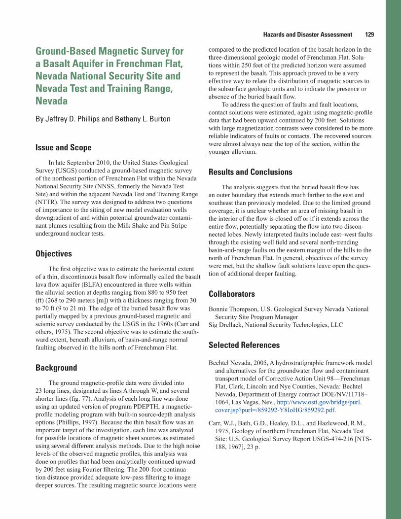
Hazards and Disaster Assessment 129
Ground-Based Magnetic Survey for a Basalt Aquifer in Frenchman Flat, Nevada National Security Site and Nevada Test and Training Range, Nevada
By Jeffrey D. Phillips and Bethany L. Burton
Issue and Scope
In late September 2010, the United States Geological Survey (USGS) conducted a ground-based magnetic survey of the northeast portion of Frenchman Flat within the Nevada National Security Site (NNSS, formerly the Nevada Test Site) and within the adjacent Nevada Test and Training Range (NTTR). The survey was designed to address two questions of importance to the siting of new model evaluation wells downgradient of and within potential groundwater contami-nant plumes resulting from the Milk Shake and Pin Stripe underground nuclear tests.
Objectives
The first objective was to estimate the horizontal extent of a thin, discontinuous basalt flow informally called the basalt lava flow aquifer (BLFA) encountered in three wells within the alluvial section at depths ranging from 880 to 950 feet (ft) (268 to 290 meters [m]) with a thickness ranging from 30 to 70 ft (9 to 21 m). The edge of the buried basalt flow was partially mapped by a previous ground-based magnetic and seismic survey conducted by the USGS in the 1960s (Carr and others, 1975). The second objective was to estimate the south-ward extent, beneath alluvium, of basin-and-range normal faulting observed in the hills north of Frenchman Flat.
Background
The ground magnetic-profile data were divided into 23 long lines, designated as lines A through W, and several shorter lines (fig. 77). Analysis of each long line was done using an updated version of program PDEPTH, a magnetic-profile modeling program with built-in source-depth analysis options (Phillips, 1997). Because the thin basalt flow was an important target of the investigation, each line was analyzed for possible locations of magnetic sheet sources as estimated using several different analysis methods. Due to the high noise levels of the observed magnetic profiles, this analysis was done on profiles that had been analytically continued upward by 200 feet using Fourier filtering. The 200-foot continua-tion distance provided adequate low-pass filtering to image deeper sources. The resulting magnetic source locations were
compared to the predicted location of the basalt horizon in the three-dimensional geologic model of Frenchman Flat. Solu-tions within 250 feet of the predicted horizon were assumed to represent the basalt. This approach proved to be a very effective way to relate the distribution of magnetic sources to the subsurface geologic units and to indicate the presence or absence of the buried basalt flow.
To address the question of faults and fault locations, contact solutions were estimated, again using magnetic-profile data that had been upward continued by 200 feet. Solutions with large magnetization contrasts were considered to be more reliable indicators of faults or contacts. The recovered sources were almost always near the top of the section, within the younger alluvium.
Results and Conclusions
The analysis suggests that the buried basalt flow has an outer boundary that extends much farther to the east and southeast than previously modeled. Due to the limited ground coverage, it is unclear whether an area of missing basalt in the interior of the flow is closed off or if it extends across the entire flow, potentially separating the flow into two discon-nected lobes. Newly interpreted faults include east–west faults through the existing well field and several north-trending basin-and-range faults on the eastern margin of the hills to the north of Frenchman Flat. In general, objectives of the survey were met, but the shallow fault solutions leave open the ques-tion of additional deeper faulting.
Collaborators
Bonnie Thompson, U.S. Geological Survey Nevada National Security Site Program ManagerSig Drellack, National Security Technologies, LLC
Selected References
Bechtel Nevada, 2005, A hydrostratigraphic framework model and alternatives for the groundwater flow and contaminant transport model of Corrective Action Unit 98—Frenchman Flat, Clark, Lincoln and Nye Counties, Nevada: Bechtel Nevada, Department of Energy contract DOE/NV/11718–1064, Las Vegas, Nev., http://www.osti.gov/bridge/purl.cover.jsp?purl=/859292-Y8IoHG/859292.pdf.
Carr, W.J., Bath, G.D., Healey, D.L., and Hazlewood, R.M., 1975, Geology of northern Frenchman Flat, Nevada Test Site: U.S. Geological Survey Report USGS-474-216 [NTS-188, 1967], 23 p.

130 Developing Integrated Methods to Address Complex Resource and Environmental Issues
Figure 77. Raw magnetic-profile data after removal of the diurnal field plotted as colored dots on a hydrostratigraphic-unit base map (Bechtel Nevada, 2005) with alluvial units above the basalt removed. The long lines are labeled by their letter designations. Of interest are the red and orange values along lines L, M, F, G, and H, which are known to be due to a discontinuous buried basalt flow encountered in nearby wells (as predicted by the dark-gray areas on the map). The red and orange values along lines I, J, K, C, P, and Q suggest that the basalt is also present over a large area of the basin to the southeast of the well control (as predicted by the light-gray areas on the geologic map).
Total magnetic field anomaly, in nanoTesla
36°50'
36°51'
36°52'
36°53'
36°54'
−115°58' −115°57' −115°56' −115°55' −115°54' −115°53'
Line R
Line S
Line U
Line V
Line I
Line K
Line
A
Line
N Line
B
Line
O
Line J
Line H
Line E
Lin
e Q
Lin
e P
Lin
e W
Line D
Line M
Line F
Line C
Line L
Line G
Line T
Line R
Line S
Line U
Line V
Line I
Line K
Line
A
Line
N Line
B
Line
O
Line J
Line H
Line E
Lin
e Q
Lin
e P
Lin
e W
Line D
Line M
Line F
Line C
Line L
Line G
Line T
0 260175 −20 20−60 60−40 40
EXPLANATION
0 1 KILOMETERS
0 1 MILES

Hazards and Disaster Assessment 131
Phillips, J.D., 1997, Potential-field geophysical software for the PC, version 2.2: U.S. Geological Survey Open-File Report 97–725, 34 p., http://pubs.usgs.gov/of/1997/ofr-97-0725/pfofr.htm.
Phillips, J.D., Burton, B.L., Curry-Elrod, Erika, and Drellack, Sigmund, 2011, A ground-based magnetic survey of French-man Flat, Nevada National Security Site and Nevada Test and Training Range, Nevada—Preliminary results: Under-ground Test Area (UGTA) Technical Information Exchange Meeting, Las Vegas, Nevada, April 27, 2011, 1 p.
Phillips, J.D., Burton, B.L., Curry-Elrod, Erika, and Drel-lack, Sigmund, 2014, A ground-based magnetic survey of Frenchman Flat, Nevada National Security Site and Nevada Test and Training Range, Nevada—Data release and pre-liminary interpretation: U.S. Geological Survey Open-File Report 2014–1187, 144 p., 1 pl., http://dx.doi.org/10.3133/ofr20141187, http://pubs.usgs.gov/of/2014/1187/.
Estimating Bedrock Depth Using Constrained Gravity Inversion, Tooele Army Depot, Utah
By Jeffrey D. Phillips and Theodore Asch
Issue and Scope
The configuration of the bedrock under the Tooele Army Depot (TEAD), Tooele, Utah, helps to contain one or more contaminant plumes of saline groundwater. These plumes are considered to be environmental hazards by the U.S. Environ-mental Protection Agency. Knowledge of the bedrock surface comes from boreholes and gravity inversion. The U.S. Geolog-ical Survey (USGS) was asked to modify a contractor’s report on the configuration of the bedrock surface following the drilling of additional boreholes and the collection of additional gravity stations at TEAD. Although the contractor’s final grid of the bedrock surface was provided to the USGS, the method-ology used by the contractor was not well documented.
Objectives
The objective of the study was to estimate the thickness of the overburden and the elevation of the bedrock surface using gravity inversion, while at the same time, forcing the result to agree with the available borehole data. The boreholes are concentrated over a bedrock high in the center of the study area, but there are scattered boreholes throughout the study area, many of which do not reach the bedrock surface. The bedrock also outcrops along the southern boundary of the study area.
Background
A critical early step in the inversion involved the removal of the regional gravity field from the complete Bouguer anomaly (CBA) data. In the absence of other information, we assumed that the regional field was represented by a planar surface over the area of interest. To determine the parameters of this regional field, we used the only information available, the known depth to bedrock in 49 boreholes and at 4 outcrop locations. A density of 2.20 grams per cubic centimeter (g/cm3) was assumed for the overburden and a density of 2.67 g/cm3 was assumed for the bedrock. The known depth to bedrock was translated into an estimated overburden gravity anomaly at the 53 locations using the Bouguer slab approximation
g hh
z == −0 012780 006007..
∆ρ
(6)
where h is the depth to bedrock in feet and Δρ is the density contrast of –0.47 g/cm3. The estimated overburden gravity

132 Developing Integrated Methods to Address Complex Resource and Environmental Issues
was subtracted from the observed CBA to give estimates of the regional gravity field at the 53 locations. A planar sur-face was then fit to these 53 estimates of regional gravity using a linear least-squares approach. This planar surface was assumed to represent the regional gravity field, and it was subtracted from the gridded CBA data to produce the observed residual gravity anomaly grid.
The gravity inversion was done using a modified Cordell-Henderson approach (Cordell and Henderson, 1968). In this approach an initial overburden thickness model, based on the Bouguer slab approximation, is modified in an itera-tive way to improve the agreement between the calculated gravity field of the model and the observed residual grav-ity field. The initial thickness estimate and a fixed nega-tive density contrast are used to calculate the gravity field of the model on a flat surface representing the top of the overburden. The calculated gravity field should be negative, except in areas where the overburden has zero thickness. If the calculated field is not negative, a minimum constant is subtracted so as to make it negative. At each iteration, the overburden thickness is updated as
new thickness observed gravity
calculated gravityold_ _
_=
× __ thickness
(7)
Usually only a few iterations are needed to bring the thickness and observed gravity into agreement.
In the modified Cordell-Henderson approach, the initial Bouguer slab thickness estimate for iteration zero and the thickness estimates for subsequent iterations calculated using equation 7 are modified to agree with the borehole data before each new gravity field is calculated. This is done using a correction surface constructed as follows from data at the borehole locations. First, the preliminary overburden thickness grid produced by equation 7 is sampled at the locations of the boreholes and outcrops. Differences between the true bedrock depths (where known) or minimum bed-rock depths (as represented by the total depths of boreholes that did not intersect bedrock) and the sampled values are computed. For boreholes (or outcrops) that intersect the bedrock surface, the difference is retained regardless of sign. For boreholes that do not intersect the bedrock surface, the difference is retained if it is negative (the preliminary surface is above the bottom of the borehole) and set to zero if it is positive (the preliminary surface is below the bottom of the borehole). The edited difference is then gridded using minimum curvature to produce the correction surface. This correction surface is added to the preliminary overburden thickness grid to produce the revised overburden thickness grid at each iteration.
Following iteration one, additional iterations did not produce any real improvement to the result (table 6), so the overburden thickness estimate from iteration one was added to the topographic surface grid generated from the 2 arc-second digital elevation model to produce the final estimated bedrock surface elevation (fig. 78).
Results and Conclusions
The final thickness estimate included undulations north of the mountain front in the southeast corner of the area. These undulations are largely unconstrained by any gravity or borehole data. The gravity field calculated from the final thickness estimate was in good agreement with the observed residual gravity, having a root-mean-squared (RMS) misfit of 0.59 milligal (mGal) (table 6). This surface is likely to be unreliable in the southwest and northwest corners and else-where where borehole data is absent and the gravity stations are sparse. Based on these results, the U.S. Army Corp of Engineers made significant modifications to their groundwater model and later performed verification drilling.
Collaborators
Karl Cole, U.S. Army Corp of Engineers
Reference Cited
Cordell, Lindrith, and Henderson, R.G., 1968, Iterative three-dimensional solution of gravity anomaly data using a digital computer: Geophysics, v. 33, p. 596–601.
Table 6. Results of modified Cordell-Henderson gravity inversion.
[RMS, root-mean-squared; mGal, milligal]
Iteration
Misfit in overburden thickness at bedrock boreholes and outcrops Gravity RMS
misfit (mGal)Mean
(feet)Standard deviation
(feet)0 –5.4 12.6 0.841 –6.6 15.3 0.592 –5.1 13.9 0.613 –5.0 15.3 0.604 –5.4 16.1 0.60

Hazards and Disaster Assessment 133
Borehole above bedrock
Borehole to bedrock
Bedrock outcrop
3,556 3,760 3,841 3,898 3,941 3,985 4,050 4,124 4,192 4,263 4,382 4,511 4,740
EXPLANATION
Estimated bedrock elevation, in feet
40°31'
40°32'
40°33'
40°34'
40°35'
−112°25' −112°24' −112°23' −112°22' −112°21' −112°20' −112°19'
3300
3400
3500
3600
3700
3800
North American Datum of 1983Utah state plane projection, central zone
Bedrock elevation, contour interval = 50 feet
4200
4300
4400
4000
3800
4300
4700
4700
5200460045
00
4100
4100
3900
4000
4200
4300
4600
4400
37003800
39004000
3900
3900
3800 3700
4100
0 1 KILOMETERS
0 1 MILES
Figure 78. Bedrock elevation for the Tooele Army Depot, Tooele, Utah, as estimated using constrained gravity inversion. The solution is colored within 1,500 feet of outcrops, boreholes, and gravity stations. Note the nonlinear color scale. Reliability is expected to be poor in the uncolored areas.

134 Developing Integrated Methods to Address Complex Resource and Environmental Issues
Development of the ALLTEM, an Electromagnetic System for Detection and Discrimination of Munitions and Explosives of Concern
By Craig W. Moulton, Theodore H. Asch, David L. Wright, David V. Smith, Paul H. Wigton, and Ronnie D. Coffee
Issue and Scope
There are hundreds of thousands of acres of Federal land that are contaminated by munitions and explosives of concern (MEC) including unexploded ordnance (UXO) and ordnance debris. Congress has mandated that formerly used target and bombing ranges be cleaned up and given back to civilian use, if possible. One mission of the U.S. Geologi-cal Survey (USGS) is to support other Federal agencies in managing national resources and protecting environmental health. The Department of Defense (DoD) Strategic Envi-ronmental Research and Development Program (SERDP) and Environmental Security and Technology Certification Program (ESTCP) have funded a project to conduct novel research whose goal is reducing remediation costs and increasing the confidence level of UXO clearance opera-tions. MEC includes items of widely varying size, from 20 millimeter (mm) projectiles to large bombs that are buried at varying depths, from the surface to many feet deep, with unknown orientations in the earth and with varying electro-magnetic and magnetic properties. Although existing electro-magnetic induction (EMI) and magnetometer sensors have demonstrated high detection rates under many conditions, the ability to discriminate between harmless buried metal objects and UXO is extremely limited.
Objectives
The U.S. Geological Survey (USGS) designed, built, and tested the ALLTEM (ALL-the-Time-ElectroMagnetic), a novel EMI system for UXO detection and discrimination. Two main design features distinguish the ALLTEM from most other EMI systems. The first is that the ALLTEM drives its transmitter loops with a continuous triangular-shaped cur-rent waveform, as opposed to a narrow time-repetitive pulse. The second is that the ALLTEM can perform UXO surveys while continuously moving as opposed to a “cued” mode of operation, requiring the system to be immobile at each data measurement point.
Figure 79. ALLTEM (ALL-the-Time-ElectroMagnetic) transmitter triangular waveform and measured responses from steel (ferrous) and brass (nonferrous) balls.
−15
−10
−5
0
5
10
15
−0.8
−0.6
−0.4
−0.2
0
0.2
0.4
0.6
0.8
0 0.001 0.002 0.003 0.004 0.005 0.006 0.007 0.008 0.009 0.01 0.011
Resp
onse
, in
volts
Time, in seconds
Exci
tatio
n cu
rren
t, in
am
ps
4-inch steel ball(ferrous)
4-inch brass ball(nonferrous)
Excitationcurrent
Background
The ALLTEM system transmitter loops are driven by a continuous triangle current waveform (fig. 79). The result-ing electromagnetically induced target-response voltages in the Rx-(receiver) induction loops are measured in the time domain. The use of a triangular wave drive in EMI systems was originally pioneered to detect large underground ore bodies (West and others, 1984) and was adapted for use in the ALLTEM (Wright and others, 2006). The use of a triangle wave has advantages over systems that use a pulse drive. One advantage is that the dynamic-range demands on the receiver electronics are smaller. Another is that ferrous and nonferrous targets show distinctly different waveforms (fig. 79).
Beyond detection of metal objects, the ability to discrimi-nate between UXO and non-UXO targets (typically metallic clutter) is a highly prized goal because in many cases more than 70 percent of range clearance costs are attributed to dig-ging up harmless scrap metal that could have been left in the ground. The ALLTEM has 19 unique combinations of drive and receiver coil measurements of the target’s response that help considerably in the data analysis process to discriminate between UXO and clutter.
The ALLTEM employs a 1-meter (m) cube containing the 3-axis drive coils, 8 pairs of small gradiometer receiver coils, and a larger, top-to-bottom, gradiometer receiver coil pair (fig. 80A). The cube and cart used to transport the cube during surveys are constructed from lightweight plastic honeycomb with fiberglass faces. The cart, with nonmetallic wheels and bearings, is connected by a 3-m fiberglass tow bar to a small tractor. The coil drive amplifier and data acquisi-tion system are housed in an electronics chassis on the back of the tractor (fig. 80B). Alternating current (AC) power for

Hazards and Disaster Assessment 135
Figure 80. ALLTEM (ALL-the-Time-ElectroMagnetic) system. A, Parts and components of the cube and cart. B, Performing a survey at Camp Stanley, Texas. (USGS photographs)
GPS guidancemonitor
2-kilowattgenerator
Transport tractor
ALLTEM cart and cube
Electronics chassisData aquisition monitor
GPS guidancemonitor
2-kilowattgenerator
Transport tractor
ALLTEM cart and cube
Electronics chassisData aquisition monitor
B
A
Z calibration ball holder
Small sensor coil (1 of 16)
X drive coil (on back)
Y calibration ball holder
ALLTEM cartALLTEM cubeY drive coil
Z drive coil
Fiberglass tow bar
Attitude sensor GPS antenna
1-meter sensor coil (under lid)
Z calibration ball holder
Small sensor coil (1 of 16)
X drive coil (on back)
Y calibration ball holder
ALLTEM cartALLTEM cubeY drive coil
Z drive coil
Fiberglass tow bar
Attitude sensor GPS antenna
1-meter sensor coil (under lid)
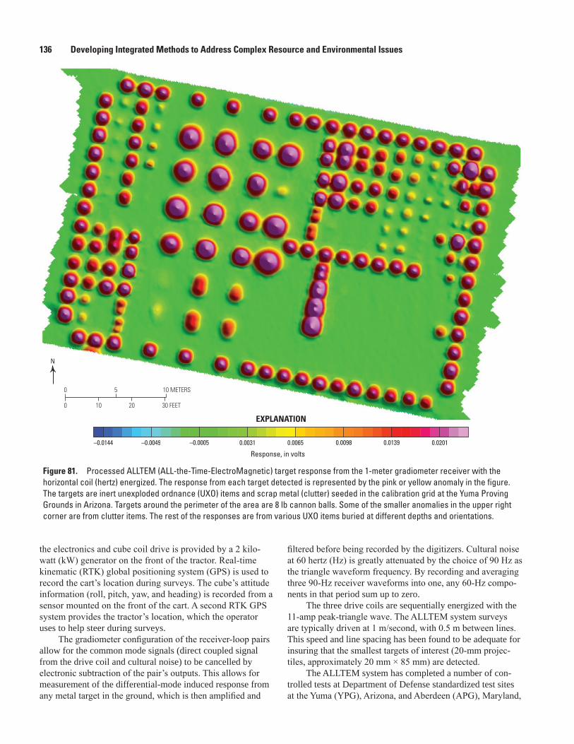
136 Developing Integrated Methods to Address Complex Resource and Environmental Issues
Figure 81. Processed ALLTEM (ALL-the-Time-ElectroMagnetic) target response from the 1-meter gradiometer receiver with the horizontal coil (hertz) energized. The response from each target detected is represented by the pink or yellow anomaly in the figure. The targets are inert unexploded ordnance (UXO) items and scrap metal (clutter) seeded in the calibration grid at the Yuma Proving Grounds in Arizona. Targets around the perimeter of the area are 8 lb cannon balls. Some of the smaller anomalies in the upper right corner are from clutter items. The rest of the responses are from various UXO items buried at different depths and orientations.
–0.0144 –0.0049 –0.0005 0.0031 0.0065 0.0098 0.0139 0.0201
EXPLANATION
Response, in volts
N
0 10 METERS5
0 10 20 30 FEET
the electronics and cube coil drive is provided by a 2 kilo-watt (kW) generator on the front of the tractor. Real-time kinematic (RTK) global positioning system (GPS) is used to record the cart’s location during surveys. The cube’s attitude information (roll, pitch, yaw, and heading) is recorded from a sensor mounted on the front of the cart. A second RTK GPS system provides the tractor’s location, which the operator uses to help steer during surveys.
The gradiometer configuration of the receiver-loop pairs allow for the common mode signals (direct coupled signal from the drive coil and cultural noise) to be cancelled by electronic subtraction of the pair’s outputs. This allows for measurement of the differential-mode induced response from any metal target in the ground, which is then amplified and
filtered before being recorded by the digitizers. Cultural noise at 60 hertz (Hz) is greatly attenuated by the choice of 90 Hz as the triangle waveform frequency. By recording and averaging three 90-Hz receiver waveforms into one, any 60-Hz compo-nents in that period sum up to zero.
The three drive coils are sequentially energized with the 11-amp peak-triangle wave. The ALLTEM system surveys are typically driven at 1 m/second, with 0.5 m between lines. This speed and line spacing has been found to be adequate for insuring that the smallest targets of interest (20-mm projec-tiles, approximately 20 mm × 85 mm) are detected.
The ALLTEM system has completed a number of con-trolled tests at Department of Defense standardized test sites at the Yuma (YPG), Arizona, and Aberdeen (APG), Maryland,

Hazards and Disaster Assessment 137
Proving Grounds. These sites consist of areas with known targets at known locations, depths, and orientations and areas with an unknown number of targets. Figure 81 shows one of the 19 target maps produced at the YPG.
The ultimate goal of this technology, as mentioned above, was to be able to discriminate between dangerous unex-ploded ordnance and harmless clutter. To meet this goal, once ALLTEM data are acquired, processed, and inverted using dipole models to represent the axial-symmetric targets of inter-est, the data are “classified” into groups of clutter and types of UXO. This is achieved by statistically comparing the proper-ties and inverted results of unknown targets to known targets. The data presented in figure 82 are an illustration of the ability of the ALLTEM data analysis to distinguish between clutter and different types of ordnance.
Results and Conclusions
The ALLTEM system has been successful in collecting high-quality target data and determining the location, depth, size, length, width, and orientation of the targets. The mod-eled target characteristics were compared to those of known UXO items to make the determination as to whether the item was UXO or not. These results have been scored by the Department of Defense (SERDP and ESTCP) and ALLTEM achieved high scores for target detection, classification
(UXO or non-UXO), and correct identification of UXO items. The ALLTEM has moved on to investigating active sites, including the Camp Stanley Storage Activity north of San Antonio, Texas, where MEC remediation efforts are cur-rently in progress.
Collaborators
Department of Defense Strategic Environmental Research and Development ProgramDepartment of Defense Environmental Security Technology Certification ProgramColorado School of Mines, Golden, Colorado
References Cited
West, G.F., Macnae, J.C., and Lamontagne, Y., 1984, A time-domain electromagnetic system measuring the step response of the ground: Geophysics, v. 49, p. 1010–1026.
Wright, D.L., Moulton, C.W., Asch, T.H., Brown, P.J., Hutton, S.R., Nabighian, M.N., and Li, Y., 2006, ALLTEM for UXO applications—First field tests: Proceedings of the Sympo-sium on the Application of Geophysics to Engineering and Environmental Problems, April 2–6, 2006, p. 1761–1775.
Figure 82. Classified ALLTEM (ALL-the-Time-ElectroMagnetic) data from Yuma Proving Ground, Arizona. Symbols represent the groupings of different munitions detected and analyzed. mm, millimeters.
0
0.01
0.02
0.03
0.04
0.05
0.06
0.07
0 0.02 0.04 0.06 0.08 0.1 0.12 0.14 0.16 0.18 0.2
Radi
us, i
n m
eter
s
Length, in meters
25 mm37 mm105M60
81mm60 mm
20 mmClutter8lb Shot105HEAT
EXPLANATION

138 Developing Integrated Methods to Address Complex Resource and Environmental Issues
Development of a Ground-Based Tensor Magnetic Gradiometer System
By David V. Smith, Robert E. Bracken, S. Ray Hutton, and Jeffrey D. Phillips
Issue and Scope
Hundreds of thousands of acres of Federal land are contaminated with ordnance debris and unexploded ordnance (UXO). Congress has mandated that formerly used target and bombing ranges be cleaned up and returned to civilian use, if at all possible. One mission of the U.S. Geological Survey (USGS) is to support other Federal agencies in managing national resources and protecting environmental health. The Strategic Environmental Research and Development Program (SERDP) funded a project to conduct novel research whose goal is reducing remediation costs and increasing the confi-dence level of clearance operations. This project draws on years of USGS expertise in research and development of pro-totype geophysical instrumentation that pushes performance envelopes and expands capabilities of potential field methods.
Objectives
The USGS designed, fabricated, tested, and evaluated a tensor magnetic gradiometer system (TMGS) for application to detection, location, and discrimination of UXO, shown in figure 83. Tensor magnetic gradiometry offers many advan-tages over scalar potential field methods. By directly measuring the gradients of the vector components of the magnetic field at a single measurement point, it is possible to determine the dis-tance and direction to a magnetic dipole source. Isolated scraps of metal and intact UXO closely approximate a dipole source; therefore, a functional TMGS potentially offers advantages over conventional magnetic surveys.
Background
Conventional magnetic sensors measure either the total magnetic field or a single magnetic vector. For these types of sensors to be successful, numerous measurements must be acquired at closely spaced locations over the survey area. As part of research into volcanic hazards, the USGS developed a portable volcano-magnetic observatory to measure subtle mag-netic field variations caused by transitions of magma through the curie-temperature. The triaxial fluxgate magnetometers from this volcano-magnetic observatory were adapted for use on a towed platform. Four observatory-grade magnetometer heads were affixed to a telescope mirror blank for dimensional stability to create the array. The array was mounted on a towed platform along with thermometers, inclinometers, and acceler-ometers to measure platform temperature, attitude, and shock and vibration (fig. 84). The data acquisition system, guidance
system, and power supplies were mounted on a tractor that towed the sensor array (fig. 83). A single magnetometer head contains three orthogonally mounted fluxgate magnetometer cores. Because of manufacturing tolerances, the cores in each head are not exactly aligned. Small, but non-negligible inor-thogonalities remain. Furthermore, offsets and misalignments exist among the four heads in the array. In order to remove the intrinsic errors caused by these misalignments, it was neces-sary to measure them through a rigorous calibration procedure using an apparatus that spun the array through a uniform magnetic field (fig. 85). Deviations from ideal responses were analyzed to yield calibration coefficients that could be used to correct the systematic errors.
Controlled tests were conducted at the Standard-ized Test Site at Yuma Proving Ground, Arizona. This test site consists of a calibration grid, a blind test grid, and an open field area. The calibration grid—a rectangular grid of 2 meters (m) by 2 m cells—contains known targets at known locations, depths, and orientations for the purpose of defin-ing system responses to UXO and non-UXO items. A similar area, the blind test grid, is seeded with targets whose loca-tions, depths, and types are unknown to experimentalists. Measurements were collected from all sensors at a rate of 1,000 hertz (Hz) as the system moved along closely spaced parallel survey lines. Accurate positions were obtained at a rate of 20 Hz using a Leica 1200 global positioning system. To account for system drift, a spin-calibration was per-formed at the beginning and end of each completed survey. Due in part to the great quantity of data obtained and subtle interactive effects of the systematic errors, extensive pro-cessing was required to extract the 81 necessary calibration coefficients and to apply these to the magnetic vector mea-surements. The final compensated data were used to create maps of tensor gradients and tensor magnitude.
Results and Conclusions
The prototype TMGS successfully acquired high-quality data in controlled tests, as shown in the tensor gradient data (fig. 86A) and tensor magnitude data (fig. 86B). The rainbow color scale registers high magnetic gradient values as red and low values as blue. This research showed that, though a TMGS can outperform competing magnetometer systems, a practical system would have to have greater signal-to-noise figures and be more stable electronically. Following the demonstration of the TMGS, research was conducted into the possibility of modifying the TMGS to incorporate a large primary coil to generate an oscillating magnetic field that would induce a controlled magnetic response in ferrous targets underlying the array. This research showed that such a system would have the ability to discriminate between intact, axially symmetric UXO and irregularly shaped pieces of scrap metal. However, such a system was deemed to be not feasible, because the engineering requirements cannot be met with existing magnetometers and materials.

Hazards and Disaster Assessment 139
Figure 85. Calibration coefficients were derived from measurements made as the magnetometer array was spun on a turntable apparatus in a nearly uniform magnetic field on site. (USGS photograph)
Figure 84. Multiaxis magnetometer array is mounted in a towed platform, along with thermometers, inclinometers, and accelerometers. (USGS photograph)
Figure 83. Tensor magnetic gradiometer system undergoing tests at Yuma Proving Ground, Arizona. (USGS photograph)

140 Developing Integrated Methods to Address Complex Resource and Environmental Issues
Figure 86. High-quality data acquired by the prototype tensor magnetic gradiometer system. A, Tensor magnetic gradient data and B, tensor magnitude data over a test site seeded with inert unexploded ordnance targets and clutter items. nT/m, nano-tesla per meter; TMGS, tensor magnetic gradiometer system.
−114.246732.8530
32.8529
32.8528
32.8527
32.8526
−114.2466 −114.2465 −114.2464 −114.2463A
B−114.2467
32.8530
32.8529
32.8528
32.8527
32.8526
−114.2466 −114.2465 −114.2464 −114.2463
EXPLANATION
EXPLANATION
−348.9−152.9
−61.3−32.8−19.3−12.0
−7.6−4.7−2.7−1.1
0.31.83.55.78.5
12.920.235.177.2
308.5
Gxx, (n T /m )
5.36.68.6
10.612.614.917.520.624.328.934.942.753.568.489.6
121.3173.6285.6566.6
1872.2
I1, (n T /m )
Collaborators
Strategic Environmental Research and Development Program (SERDP)

Hazards and Disaster Assessment 141
U.S. Geological Survey Environmental Studies of the World Trade Center Area, New York City, after September 11, 2001
By Roger N. Clark and Gregg A. Swayze
Issue and Scope
The U.S. Geological Survey (USGS) response to the World Trade Center disaster illustrates the integrated capa-bilities of imaging spectroscopy, field work, and laboratory analyses. Two days after the September 11, 2001, attack on World Trade Center (WTC), the USGS was asked by the U.S. Environmental Protection Agency (EPA) and the U.S. Public Health Service to conduct a remote-sensing and mineralogi-cal characterization study of lower Manhattan around the WTC. This study, conducted in cooperation with the National Aeronautics and Space Administration (NASA) and the Jet Propulsion Laboratory (JPL), was requested to rapidly provide emergency response teams with information on the concentra-tions and distribution of asbestos and other materials in the dusts deposited around lower Manhattan after the September 11 WTC building collapse in New York City.
Objectives
The airborne visible/infrared imaging spectrometer (AVIRIS), an aircraft-based remote-sensing instrument, was flown by JPL/NASA over the WTC area on September 16, 18, 22, and 23, 2001. From September 16 through 19, 2001, a two-person USGS field crew visited lower Manhattan to field calibrate the AVIRIS remote sensing and collect samples of dust and airfall debris from 33 outdoor locations within a 1-kilometer radius of the WTC. The objectives were to charac-terize the extent and hazards created by the disaster.
Background
AVIRIS remote sensing measures the amount of light reflected from the ground surface in the visible through near-infrared spectrum. Individual minerals or other dust components have characteristic light reflection features across the visible and infrared spectrum, which can be used to map spatial variations in the materials making up the dusts depos-ited around the WTC.
Samples of the dusts were analyzed using several differ-ent methods. All of the results indicate that the dust deposits formed from the WTC collapse are heterogeneous and are composed largely of particles of glass fibers, gypsum wall-board, concrete, paper, window glass, and other miscellaneous materials commonly used in building construction or found in office buildings.
Results and Conclusions
AVIRIS was used to detect high-temperature fires burn-ing within the debris through smoke because first responders could not see the fires deep within the debris pile (fig. 87). The AVIRIS data were used to find location, temperature, and size of the hot spots on September 16, 18, 22, and 23, 2001 (see Clark, Green, Swayze, Hoefen, and others, 2001; Clark, Green, Swayze, Meeker, and others, 2001; Clark and others, 2006).
The USGS detected chrysotile asbestos in more than two thirds of the dust samples studied, at levels less than 1 weight percent. Analyses of the material coating a steel beam in the WTC debris detected the presence of chrysotile asbes-tos at levels as high as 20 percent (by volume) of the coating material. See Clark, Green, Swayze, Meeker, and others, 2001 (2001), Meeker and others (2006), Plumlee and others (2006), and Swayze and others (2006) for more details.
Collaborators
National Aeronautics and Space Administration (NASA)Environmental Protection Agency (EPA)
Primary Products
Materials maps of minerals, organics, and other com-pounds. Maps of thermal hot spots and their global positioning system (GPS) locations as shown here in this report.
References Cited
Clark, R.N., Green, R.O., Swayze, G.A., Hoefen, T.M., Livo, K.E., Pavri, Betina, Sarcher, Chuck., Boardman, Joe, and Vance, J.S., 2001a, Images of the World Trade Center site show thermal hot spots on September 16 and 23, 2001: U.S. Geological Survey Open-File Report 01–0405, unpaged, http://pubs.usgs.gov/of/2001/ofr-01-0405/.
Clark, R.N., Green, R.O., Swayze, G.A., Meeker, Greg, Sutley, Steve, Hoefen, T.M., Livo, K.E., Plumlee, Geoff, Pavri, Betina, Sarture, Chuck, Wilson, Steve, Hageman, Phil, Lamothe, Paul, Vance, J.S., Boardman, Joe, Brown-field, Isabelle, Gent, Carol, Morath, L.C., Taggart, Joseph, Theodorakos, P.M., and Adams, Monique, 2001b, Envi-ronmental studies of the World Trade Center area after the September 11, 2001, attack: U. S. Geological Survey Open File Report 01–0429, [about 260 printed] p., http://pubs.usgs.gov/of/2001/ofr-01-0429/.

142 Developing Integrated Methods to Address Complex Resource and Environmental Issues
WTCsite
EXPLANATION
Color infrared composite: Blue = 0.56 microns Green = 1.59 microns Red = 2.47 microns
0 200 METERS
0 200 FEET
N
0 100 METERS
0 100 FEET

Hazards and Disaster Assessment 143
Clark, R.N., Swayze, G.A., Hoefen, T.M., Green, R.O., Livo, K.E., Meeker, G.P., Sutley, S.J., Plumlee, G.S., Pavri, Betina, Sarture, Chuck, Boardman, Joe, Brownfield, I.K., and Morath, L.C., 2006, Environmental mapping of the World Trade Center area with imaging spectroscopy after the September 11, 2001 attack, chap. 4, Gaffney, J.S., and Marley, N.A. (eds.), Urban aerosols and their impacts—Lessons learned from the World Trade Center tragedy: Oxford University Press, American Chemical Society, Symposium Series 919, p. 66–83, plates 4.1–4.6.
Meeker, G.P., Sutley, S.J., Brownfield, I.K., Lowers, H.A., Bern, A.M., Swayze, G.A., Hoefen, T.M., Plumlee, G.S., Clark, R.N., and Gent, C.A., 2006, Materials characteriza-tion of dusts generated by the collapse of the World Trade Center, chap. 5, Gaffney, J.S. and Marley, N.A. (eds.), Urban aerosols and their impacts—Lessons learned from the World Trade Center tragedy: Oxford University Press, American Chemical Society, Symposium Series 919, p. 84–102.
Figure 87 (facing page). False-color images showing the core affected area around the World Trade Center (WTC) extending from 5 to 12 days after the collapse. Hot spots appear orange and yellow. Dozens of hot spots are seen September 16 and 18, 2001, but most had cooled or the fires had been put out by September 23. The September 18 image is dark because of clouds that blocked sunlight but not light emitted by the fires. The explanation shows hot-spot locations (A–J) in table I of Clark and others (2006). Analysis of the data indicates temperatures greater than 700 °C. More than three dozen hot spots are identified in the core zone. By September 23, only four, or possibly five, hot spots are apparent in the image, with temperatures cooler than those on September 16. Vegetated areas are green, water is blue, and the smoke from the fires appears as a light-blue haze. White and lighter blue areas are rooftops, roads, and concrete as well as dust and debris from the collapsed buildings. Dust, probably more than a few millimeters thick (the optical depth), appears in shades of brown around the core WTC area on September 16.
Plumlee, G.S., Hageman, P.L., Lamothe, P.J., Ziegler, T.L., Meeker, G.P., Theodorakos, P.M., Brownfield, I.K., Adams, M.G., Swayze G.A., Hoefen, T.M., Taggart, J.E., Clark, R.N., Wilson, S.E., and Sutley, S.J., 2006, Inorganic chemi-cal composition and chemical reactivity of settled dusts generated by the World Trade Center building collapse, chap. 12, Gaffney, J.S. and Marley, N.A. (eds.), Urban aero-sols and their impacts—Lessons learned from the World Trade Center tragedy: Oxford University Press, American Chemical Society, Symposium Series 919, p. 238–276, plates 12.1–12.2.
Swayze, G.A., Clark, R.N., Sutley, S.J., Hoefen, T.M., Plumlee, G.S., Meeker, G.P., Brownfield, I.K., Livo, K.E., and Morath, L.C., 2006, Spectroscopic and X-ray diffrac-tion analyses of asbestos in the World Trade Center dust, chap. 3, Gaffney, J.S. and Marley, N.A. (eds.), Urban aero-sols and their impacts—Lessons learned from the World Trade Center tragedy: Oxford University Press, American Chemical Society, Symposium Series 919, p. 40–65.

144 Developing Integrated Methods to Address Complex Resource and Environmental Issues
Spectral Studies of the Deepwater Horizon Oil Spill
By Gregg A. Swayze and Roger N. Clark
Issue and Scope
Remote sensing of surface oil has the potential to provide emergency responders and scientists with a tool to monitor an oil spill, remotely measure variations in its chemistry, and examine how the oil interacts with its surroundings on a large scale. Such a tool can help scientists develop insights into the fate of petroleum in the environment and whether it leaks from natural or anthropogenic sources. A rapid, quantitative, remote-sensing method is needed to map the extent of oil spills, assess their chemistry, and calculate their volume so adequate resources can be devoted to cleanup efforts.
Though satellite color-broadband imagery can show the location of surface oil, it is difficult to assess its thickness and volume with these data because it has a relatively low signal-to-noise ratio and does not contain enough information to robustly correct for interfering atmospheric aerosols and atmo-spheric gas absorptions. Alternatively, imaging spectroscopy, a relatively new type of ultraviolet to near-infrared remote sensing that measures reflected light in hundreds of contiguous spectral channels can overcome these difficulties to provide quantitative estimates of oil spill thickness and volume.
Objectives
In response to a request by National Oceanic and Atmo-spheric Administration for an estimate of the volume of oil floating on the ocean surface from the Deepwater Horizon oil spill in the Gulf of Mexico, a method of near-infrared (NIR) imaging spectroscopic analysis was developed to map the locations of thick oil floating on water (Clark and others, 2010). The method uses the shape of NIR absorption features and spectral continuum slopes due to organic compounds found in oil to identify different oil chemistries, including its weathering state and thickness. These diagnostic vibrational absorptions are too weak for detection in thin oil sheens (a few microns), but thicker (a few millimeters) water-in-oil emulsion slicks have strong detectable absorptions and are bright in the NIR compared to surrounding water (fig. 88).
Our experience in analyzing imaging spectrometer data acquired over Hurricane Katrina damaged areas of the Gulf Coast and open ocean suggested that thick crude oil emulsions could be differentiated from seaweed and algal life floating on the surface of the ocean (Swayze and others, 2007). With this experience in mind, remote-sensing data for this analysis were collected by the UV-NIR 224 spectral channel National Aero-nautics and Space Administration (NASA) airborne visible/infrared imaging spectrometer (AVIRIS) instrument, which was flown over the oil spill on May 17, 2010.
Background
Because of the large extent of the Deepwater Horizon oil spill, AVIRIS flight lines could cover only a portion of the spill on a relatively calm, nearly cloud-free day. Flight lines were oriented and timed to avoid sun glint, which complicates data analysis. The U.S. Geological Survey (USGS) Tetracorder “shape-matching” spectral identification system (Clark and others, 2003) was used to turn AVIRIS images into color-coded oil:water ratio, areal fraction, thickness, and volume maps for thick oil floating on the ocean surface within the limits of light penetration into the oil.
An emulsion sample collected on a May 7, 2010 boat traverse to the incident site (fig. 89) was used to create a series of emulsions that spanned the entire oil:water range by addi-tion of seawater or evaporation of contained water. In all, 22 reference spectra of these lab-constructed emulsions measured at thicknesses ranging from 0.025 to 28 millimeters (mm) were used for spectral mapping. The proportion of emul-sion to water covering a given pixel can be calculated based on the reflectance value (that can vary between 0 and 1) at 1.3 microns and the assumption that the spectral contribution of water at that wavelength is essentially zero.
Depending on the relative depths of oil and water-related NIR absorptions, the oil-to-water ratios of thick emulsion slicks were estimated for pixels in the AVIRIS data (fig. 90). The volume of oil in a pixel is a function of the area of the pixel, areal fraction of oil in that pixel, thickness of emulsion in that pixel, and the average oil:water ratio of the emulsion in that pixel. Values for each of these parameters were derived from the instrument flight altitude and the spectrally matching emulsion selected by Tetracorder for a given pixel. On this same day a NASA MODIS (Moderate Resolution Imaging Spectroradiometer; Terra) satellite-broadband image of the spill with a strong sun glint component was acquired from orbit. In this case sun glint helps define the boundaries and internal structure of the spill, and when compared to overlap-ping higher spatial resolution (8.5 × 8.5 meters [m] per pixel) AVIRIS data, indicates that the brownish-gray core of the spill was composed of emulsion slicks (2 percent) and broad inter-vening sheens, whereas its gray outer regions were composed entirely of sheens at the relatively coarse spatial resolution of the MODIS image (250 × 250 m/pixel).
Results and Conclusions
Tetracorder-derived lower limits for oil volumes within the top few millimeters of the ocean surface directly probed with the NIR light in the AVIRIS scenes were 19,000 (con-servative) to 34,000 (aggressive) barrels of oil. Based on laboratory measurements, NIR photons penetrate only a few millimeters into oil-water emulsions. As such, the oil vol-umes derived with this method are lower limits. Spectra of emulsions begin to resemble one another beyond a certain thickness threshold because light can only penetrate a certain depth before it is either absorbed or scattered back out of an

Hazards and Disaster Assessment 145
Figure 88. Laboratory spectra of oil:water emulsion from the Deepwater Horizon oil spill. Sample (DWH10-3) collected May 7, 2010. At visible wavelengths, the oil is very absorbing and does not change color significantly with thickness. At infrared wavelengths, both reflectance levels and absorptions due to organic compounds vary in strength with thickness. This sample contains approximately 40 percent water as determined by heat separation. Black line is for illustrative purposes to better visualize continuum endpoints used for mapping individual absorptions. From Clark and others (2010). µm, micrometers; mm, millimeters.
Visiblespectrum
4 mmthickness
0.1 mmthickness
1.2-µmC-H feature
1.73-µmC-H feature
2.3-µmC-H feature
0.6
0.5
0.4
0.3
0.2
0.1
0.00.5 1.0 1.5 2.0 2.5
Refle
ctan
ce
Wavelength, in micrometers
emulsion’s surface. The conservative and aggressive volume estimates are based on choosing either 2 millimeters (mm) (conservative) or 4 mm (aggressive) for AVIRIS spectra of sea-surface emulsions that spectrally resemble similar-looking reference emulsions with those thicknesses.
On May 17, 2010 AVIRIS covered about 30 percent of the core spill area. Areas of oil sheen lacking oil emulsion slicks outside of the core spill were not evaluated for oil volume in this study. If the core spill areas not covered by flight lines contained similar amounts of oil and water-in-oil emulsions, then extrapolation to the entire core spill area defined by the MODIS image indicates a minimum of 66,000 to 120,000 bar-rels of oil were floating on the surface. Further, the detection is only of thick surface oil and does not include oil in sheens, oil
under the surface, oil washed onto land, or oil burned, evapo-rated, or biodegraded as of May 17. These minimum surface volumes form the basis of the Mass Balance Team’s flow-rate estimates (Labson and others, 2010). Because NIR light penetration within emulsions is limited, and having made field observations that oil emulsions sometimes exceeded 20 mm in thickness, we estimate that the volume of oil, including oil thicker than can be probed in the AVIRIS imagery, is possibly as much as 150,000 barrels in the AVIRIS scenes. When this value is projected to the entire spill, it gives a volume of about 500,000 barrels of thick oil remaining on the ocean surface as of May 17. This method can be applied to future spills for esti-mating emulsion oil:water ratios and their volume to help direct recovery efforts to areas where they are most effective.

146 Developing Integrated Methods to Address Complex Resource and Environmental Issues
Figure 90 (facing page). Mapping results for oil-to-water ratio for a portion of AVIRIS (airborne visible and infra-red imaging spectrometer) flight line (May 17, 2010). The width of the scene is about 5.5 kilometers and north is at about the 4 o’clock position. Black areas on the right panel are where no thick oil was detected. The center of this image is about 12 kilometers west- southwest of the Macondo well site. From Clark and others (2010).
Figure 89. Oil emulsion from the Deepwater Horizon oil spill in the Gulf of Mexico off the Louisiana coast. Photograph taken on May 7, 2010, by Sonia Gallegos and Gregg Swayze.
Collaborators
National Aeronautics and Space Administration California Institute of Technology/Jet Propulsion Laboratory National Oceanic and Atmospheric Administration U.S. Geological Survey, Minerals and Health Project Funding provided by U.S. Coast Guard
Primary Products
We provided the first independent Federal Government estimate for the volume of oil floating on the ocean surface as of May 17, 2010. This information was used to estimate a mini-mum range flow rate for the Macondo well at between 12,500 to 21,500 barrels of oil per day for 27 days from April 20 to May 17, 2010. This flow rate implied that the Deepwater Horizon oil spill was larger than that of the Exxon Valdez as of this date.

Hazards and Disaster Assessment 147
EXPLANATIONOil:Water >90:<10
80:20 60:40 40:60 23:77 6:94 1:99~60:40
>90:<10
80:20
60:40
40:60
23:77
6:94
1:99
~60:40
A B
0 1 KILOMETERS
0 1 MILES

148 Developing Integrated Methods to Address Complex Resource and Environmental Issues
References Cited
Clark, R.N., Swayze, G.A., Leifer, Ira, Livo, K.E., Kokaly, Raymond., Hoefen, Todd, Lundeen, Sarah, Eastwood, Michael, Green, R.O., Pearson, Neil, Sarture, Charles, McCubbin, Ian, Roberts, Dar, Bradley, Eliza, Steele, Denis, Ryan, Thomas, Dominguez, Roseanne, and Air-borne Visible/Infrared Imaging Spectrometer (AVIRIS) Team, 2010, A method for quantitative mapping of thick oil spills using imaging spectroscopy: U.S. Geological Survey Open-File Report 2010–1167, 51 p., http://pubs.usgs.gov/of/2010/1167/.
Clark, R.N., Swayze, G.A., Livo, K.E., Kokaly, R.F., Sut-ley, S.J., Dalton, J.B., McDougal, R.R., and Gent, C.A., 2003, Imaging spectroscopy—Earth and planetary remote sensing with the USGS Tetracorder and Expert Systems: Journal of Geophysical Research, v. 108, no. E12, 5131, doi:10.1029/2002JE001847, 44 p., http://speclab.cr.usgs.gov/PAPERS/tetracorder/.
Labson, V.F., Clark, R.N., Swayze, G.A., Hoefen, T.M., Kokaly, Raymond, Livo, K.E., Powers, M.H., Plumlee, G.S., and Meeker, G.P., 2010, Estimated lower bound for leak rates from the Deepwater Horizon spill—Interim report to the Flow Rate Technical Group from the Mass Balance Team: U.S. Geological Survey Open-File Report 2010–1132, 4 p., http://pubs.usgs.gov/of/2010/1132/.
Swayze, G.A., Furlong, E.T., and Livo, K.E., 2007, Mapping pollution plumes in areas impacted by Hurricane Katrina with imaging spectroscopy [abs.]: American Geophysi-cal Union, v. 88, no. 52, Fall Meeting, Abstract H31L-07, http://www.agu.org/meetings/fm07/fm07-sessions/fm07_H31L.html.

Unlocking Secrets of East Antarctica with Geophysics
By Carol A. Finn
Issue and Scope
Exploration, whether for resources or knowledge of Earth and beyond, is a fundamental imperative for man. One of the least explored parts of the planet is East Antarctica whose geology and past is shrouded by the East Antarctic Ice Sheet. During the International Polar Year (IPY, 2007–2009), a team of seven nations launched an expedition to the Gamburtsev Subglacial Mountains, a hidden range the size of the European Alps. This multinational, multidisciplinary effort included aero-geophysics, traverse programs, and passive seismic instrumen-tation complimented by ice core and bedrock drilling. A central component of the Gamburtsev Mountains expedition was a major aerogeophysical survey targeted at understanding the tectonic origin of these enigmatic mountains, providing crucial new inputs into ice sheet models, identifying potential drilling sites for the international ice core community, and providing key site survey support for the Chinese ice and bedrock drilling efforts. In addition, understanding the evolution of the greater East Antarctic Precambrian shield will help constrain under-standing of the Precambrian plate reconstructions (Finn and Pisarevesky, 2007) and Cenozoic ice sheet development (Beh-rendt and others, 2007) critical to climate and resource studies.
A major new airborne dataset including gravity, magnet-ics, ice thickness, SAR (Synthetic Aperture Radar) images of the ice-bed interface, near-surface and deep internal layers, and ice-surface elevation was acquired during the IPY. The U.S. Geological Survey (USGS) is continuing its long tradi-tion—starting with the first magnetic survey ever conducted in Antarctica in 1946—of collecting, processing, and archiving the aeromagnetic data. Interpretation required innovative methods and approaches (for example, see Phillips, 1997; Phillips, 2007).
Objectives
The Gamburtsev Subglacial Mountains are important because they are thought to be the location where the ice sheet we know today initiated its march across Antarctica. Unravelling the history of the Gamburtsev Mountains pro-vides climate studies with a better understanding, not just of past changes on Earth, but possible future scenarios as well. One hundred and twenty thousand kilometers (km) of new aerogeophysical data were collected and merged with satellite
and previous airborne geophysical data resulting in data over an area of 2,000 × 1,500 km and providing the most compre-hensive geophysical perspective of crustal architecture and mountain-building processes in interior East Antarctica. The objectives of this study are to map and model geophysical data from East Antarctica and to determine models for the origin of the Gamburtsev Mountains.
Background
The Gamburtsev Subglacial Mountains are the least understood tectonic feature on Earth because they are com-pletely hidden beneath the East Antarctic Ice Sheet. Their high elevation and jagged topography are intriguing. How could such a topography, which is characteristic of recently formed and uplifted tectonic features, have formed in the interior of an ancient, geologically dead continent (Veevers, 2011)? The preservation of Alpine topography in the Gamburtsevs may reflect extremely low long-term erosion rates beneath the ice sheet but do not explain the uplift of the mountains. Analysis and modeling of the geophysical data were the first steps in unlocking the secrets of the tectonic history of these enigmatic mountains. This required application of techniques developed at the USGS including filtering, depth estimates (Finn and Ravat, 2004), equivalent source determination, and modeling (Phillips, 1992, 1997, 2000, 2001, 2007). The results from application of these techniques helped constrain modeling of the magnetic, gravity, radar, and seismic data.
Results and Conclusions
The new radar data reveal highly dissected Alpine topography reaching maximum elevations of 3,000 meters (m) and a median elevation of about 1,400 m in the north- to south-trending Gamburtsevs (fig. 91). The magnetic data distinguish several basement provinces indicating that interior East Antarctica is probably composed of a mosaic of differ-ent Precambrian cratons and orogens as in other parts of East Antarctica (Finn and others, 2006; Finn and others, 2011; Goodge and Finn, 2010). The linear, northeast-trending mag-netic anomalies that characterize much of the Gamburtsevs are similar to anomalies associated with Precambrian sources to the north. Regional northeast-trending Bouguer gravity lows and seismic data (Hansen and others, 2010) define a thickened Precambrian crust under the Gamburtsev province (fig. 91) (Ferraccioli and others, 2011).
Gravity models, constrained by seismic data (Hansen and others, 2010) and magnetic depth estimates (Phillips, 2002; Finn and Ravat, 2004), indicate an anomalously high density lower crustal root beneath the northern and central Gamburst-evs. These high densities are comparable to those modelled
Databases and Framework Studies

150 Developing Integrated Methods to Address Complex Resource and Environmental Issues
beneath old collisional orogens whose dense lower crustal roots lost buoyancy owing to temperature decreases and meta-morphism (Leech, 2001; Fischer, 2002). Precambrian ages of the Gamburtsev and Vostok provinces suggest that collisional events associated with Rodinia or earlier supercontinental assembly formed the crustal root (Ferraccioli and others, 2011) (fig. 91).
More recent tectonic events must have rejuvenated the crustal root and triggered uplift of the modern Gamburtsevs (Ferraccioli and others, 2011). Extension around 250 mil-lion years (m.y.) ago and oblique rifting ≈100 m.y. ago led to the formation of an extensive rift-valley system with uplifted flanks (Lambert rift, fig. 91). The new data reveal that the Lam-bert rift branches at the northwestern edge of the Gamburtsevs into narrow basins that surround the Gamburtsev province (fig. 91). Collectively, the rifts form part of a newly identified East Antarctic rift system, with similar geometry and length to the modern East African rift system (fig. 91). Today, these rift basins host the largest of all subglacial lakes in Antarctica
(for example, Lake Vostok, fig. 91), which resemble in size rift lakes in East Africa (Ferraccioli and others, 2011; Finn, 2011).
Mechanical unloading of the lithosphere during extension and consequent isostatic rebound produces high topography along rift flanks. The rifting enhanced the buoyancy of the crustal root by heating and possible introduction of water. The uplift of the Gamburtsevs was driven by a combination of the buoyancy of the root and the isostatic response—the readjust-ment of the level of the crustal root in the underlying mantle—to mechanical and erosional unloading of overlying rock along the rift flank and in the glacial valleys (Veevers, 2011). The uplifted regions were incised, first by rivers and then (from 34–14 m.y. ago) by glaciers, to create the steep peaks and val-leys of the Gamburtsevs. The youthful topography of the Gam-burtsevs was then literally frozen by the East Antarctic Ice Sheet ≈14 Ma (Mega-annum). The models show that the combination of rift-flank uplift, root buoyancy, and the isostatic response to fluvial and glacial erosion explain the high elevation and relief of the Gamburtsevs. The evolution of the Gamburtsevs dem-onstrates that rifting and preserved orogenic roots can produce broad regions of high topography in continental interiors without significantly modifying the underlying Precambrian lithosphere. In addition, mountain building is often attributed to a single tectonic event in contrast to the multiple events over a billion years that formed the Gamburtsevs. Any pre-existing conditions for mountain building are often unknown. Therefore, the Gamburtsevs may inform studies of other mountain ranges where a youthful look may mask a hidden past.
Collaborators
Robin Bell (Lamont-Doherty Earth Observatory)Fausto Ferraccioli (British Antarctic Survey)Detelef Damaske (German Geological Survey)John Goodge (University of Minnesota-Duluth)Tom Jordan (British Antarctic Survey)Lester Anderson (British Antarctic Survey)Mark Fahnstock (University of New Hampshire)David Braaten (University of Kansas)Adrian Smith (Lamont-Doherty Earth Observatory)Jared Abraham (U.S. Geological Survey)Eric Anderson (U.S.Geological Survey)
References Cited
Behrendt, J.C., Finn, C.A., and Blankenship, D.D., 2007, Question of ages of Cenozoic volcanic centers inferred beneath the West Antarctic Ice Sheet (WAIS) in the West Antarctic rift system (WR) from coincident aeromagnetic and radar ice sounding surveys: Eos, Transactions Ameri-can Geophysical Union, v. 88, Fall Meeting Supplement, Abstract C51A-0068.
Figure 91. Three-dimensional perspective of the Gamburtsev Subglacial Mountains, including a view of the deep root imaged beneath the range and of the thinner crust of the East Antarctic rift system that surrounds the mountains (modified from Ferraccioli and others, 2011).
- - -
GamburtsevMountains

Databases and Framework Studies 151
Ferraccioli, Fausto., Finn, C.A., Jordan, T.A., Bell, R.E., Anderson, L.M., and Damaske, Detlef., 2011, East Antarctic rifting triggers uplift of the Gamburtsev Mountains: Nature, v. 479, p. 388–394.
Finn, C.A., and Pisarevesky, S., 2007, New airborne magnetic data evaluate SWEAT reconstruction, in Antarctica., in Cooper, A.K., Raymond, C.R., and 10th ISAES Editorial Team, eds., Antarctica—A keystone in a changing world—Online proceedings of the 10th International Symposium on Antarctic Earth Sciences [abs]: U.S. Geological Survey Open-File Report 2007–1047, Extended Abstract 170, 4 p.
Finn, C.A., and Ravat, D., 2004, Magnetic depth estimates and their potential for constraining crustal composition and heat flow in Antarctica: Eos, Transactions American Geophysical Union, Fall Meeting Supplement, v. 85, Abstract T11A-1236.
Finn, C., Ferraccioli, F., and Golynsky, A., 2011, Geology of East Antarctica from a geophysical perspective—Some of the latest news [abs.]: 11th International Symposium on Antarctic Earth Sciences, July 10–15, 2011, Edinburgh, Scotland, p. 219.
Finn, C., Ferraccioli, Fausto, Jordan, Tom, Block, Adrienne, and Bell, R.E., 2011, Rift controls on the location of some large subglacial lakes in East Antarctica [abs.]: 11th Interna-tional Symposium on Antarctic Earth Sciences, July 10–15, 2011, Edinburgh, Scotland, p. 140.
Finn, C.A., Goodge, J.W., Damaske, DDetlef, and Fan-ning, C.M., 2006, Scouting craton’s edge in Paleo-Pacific Gondwana, in Fütterer, D., Damaske, D., Kleinschmidt, G., Miller, H., and Tessensohn, F., eds., Antarctica—Contributions to global earth sciences: 9th International Symposium on Antararctic Earth Sciences, Potsdam, Germany, Alfred Wegener Institute, p. 165–174.
Fischer, K.M., 2002, Waning buoyancy in the crustal roots of old mountains: Nature, v. 417, p. 933–936.
Goodge, J.W., and Finn, C.A., 2010, Glimpses of East Antarc-tica—Aeromagnetic and satellite magnetic view from the central Transantarctic Mountains of East Antarctica: Journal of Geophysical Research, v. 115, p. 22.
Hansen, S.E., Nyblade, A.A., Heeszel, D.S., Wiens, D.A., Shore, Patrick, and Kanao, Masaki, 2010, Crustal structure of the Gamburtsev Mountains, East Antarctica, from S-wave receiver functions and Rayleigh wave phase velocities: Earth and Planetary Science Letters, v. 300, p. 395–401.
Leech, M.L., 2001, Arrested orogenic development—Eclogitization, delamination and tectonic collapse: Earth and Planetary Science Letters, v. 185, p. 149–159.
Phillips, J.D., 1992, TERRACE–A terracing procedure for gridded data, with FORTRAN programs and VAX com-mand procedures, UNIX C-shell and DOS implimentations: U.S. Geological Survey Open-File Report 92–5–A–B, 20 p., 1 diskette.
Phillips, J.D., 1997, Potential-field geophysical software for the PC, version 2.2: U.S. Geological Survey Open-File Report 97–725, not paged.
Phillips, J.D., 2000, Locating magnetic contacts—A com-parison of the horizontal gradient, analytic signal, and local wavenumber methods [abs.]: Society of Exploration Geophysicists Technical Program Expanded Abstracts, p. 402–405.
Phillips, J.D., 2001, Designing matched bandpass and azi-muthal filters for the separation of potential-field anomalies by source region and source type [abs.]: Australian Society of Exploration Geophysicists, 15th Geophysical Conference and Exhibition, Expanded Abstracts CD-ROM, p. 4.
Phillips, J.D., 2002, Two-step processing for 3D magnetic source locations and structural indices using extended Euler or analytic signal methods [abs.]: Society of Explo-ration Geophysicists, 2002 Technical Program Expanded Abstracts, v. 21, p. 727–730.
Phillips, J.D., 2007, Geosoft eXecutables (GX’s) developed by the U.S. Geological Survey, version 2.0, with notes on GX development from Fortran code: U.S. Geological Survey Open-File Report 2007–1355, 111 p.
Veevers, J.J., 2011, Earth’s longest fossil rift-valley system: Nature, v. 479, p. 304–306.

152 Developing Integrated Methods to Address Complex Resource and Environmental Issues
Linking Petrophysical Properties to Environmental and Geological Factors
By Robert J. Horton and Anne E. McCafferty
Issue and Scope
The U.S. Geological Survey (USGS), in cooperation with other Federal agencies, has been investigating the nega-tive effects of acid-mine drainage in the upper Animas River watershed. Natural weathering of mineral assemblages formed from extensive hydrothermal alteration of volcanic and plutonic rocks is a significant contributor to the quality of surface and
groundwater in the watershed. Characterization of in situ rock properties related to this weathering is important to establish the background influences these rocks may have on water quality. Land managers can then use this information to develop realistic water-quality targets for cleanup efforts of mined areas.
As part of the investigation, a suite of samples were col-lected from volcanic and plutonic rocks that form the majority of exposed bedrock in the watershed (fig. 92). The samples were analyzed with a wide range of geochemical, mineralogi-cal, and geophysical laboratory methods (McCafferty and oth-ers, 2011). Laboratory measurements relate physical property values to measurements of acid neutralization capacity (ANC) and net acid production (NAP). Results have helped to develop an understanding of how chemical and physical characteristics change with alteration type for numerous rock types.
Figure 92. Geologic map of the study area with locations of samples. Descriptions of geologic units are given in table 7.
!
!
Silverton
37°55'
Tpa
Tpa
Tpa
Tpa
Tpa
Tpa
Tpa
Tpa
Tig
Tig
Tig
Tig
Tig
Tig
Tb
Tb
Tb
Tb
Tb
Tb
Tb
Tb
Tb
Tdi
Tse
Tse
Tse
Tse
Tsj
Tsj
Tsj
Tsj
107°45' 107°40' 107°35'
37°50'
pg pg
0 5 KILOMETERS1 2 3 4
0 1 2 3 4 5 MILES
Mineral Creek
Cem
ent
Cree
k
Upper
Animas
Rive
r
EXPLANATIONSample locationsAirborne magnetic and resistivity surveyStreamsWatershed boundarySilverton caldera margin—dashed where inferred
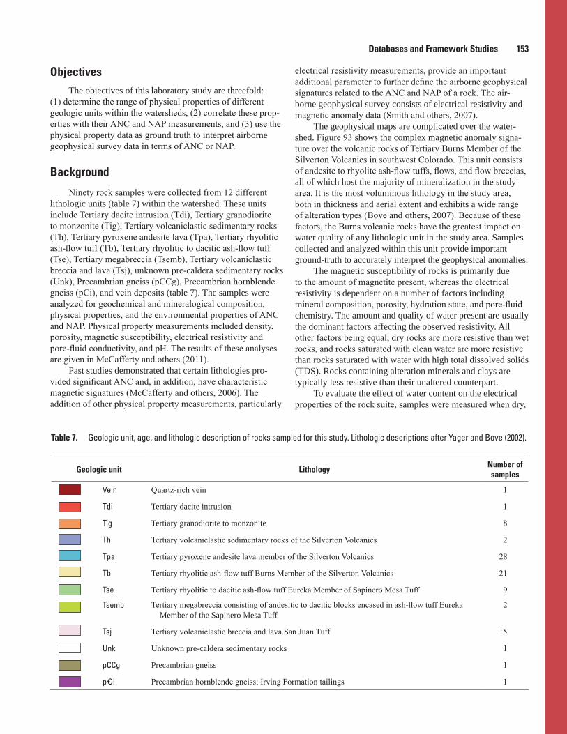
Databases and Framework Studies 153
ObjectivesThe objectives of this laboratory study are threefold:
(1) determine the range of physical properties of different geologic units within the watersheds, (2) correlate these prop-erties with their ANC and NAP measurements, and (3) use the physical property data as ground truth to interpret airborne geophysical survey data in terms of ANC or NAP.
Background
Ninety rock samples were collected from 12 different lithologic units (table 7) within the watershed. These units include Tertiary dacite intrusion (Tdi), Tertiary granodiorite to monzonite (Tig), Tertiary volcaniclastic sedimentary rocks (Th), Tertiary pyroxene andesite lava (Tpa), Tertiary rhyolitic ash-flow tuff (Tb), Tertiary rhyolitic to dacitic ash-flow tuff (Tse), Tertiary megabreccia (Tsemb), Tertiary volcaniclastic breccia and lava (Tsj), unknown pre-caldera sedimentary rocks (Unk), Precambrian gneiss (pCCg), Precambrian hornblende gneiss (pCi), and vein deposits (table 7). The samples were analyzed for geochemical and mineralogical composition, physical properties, and the environmental properties of ANC and NAP. Physical property measurements included density, porosity, magnetic susceptibility, electrical resistivity and pore-fluid conductivity, and pH. The results of these analyses are given in McCafferty and others (2011).
Past studies demonstrated that certain lithologies pro-vided significant ANC and, in addition, have characteristic magnetic signatures (McCafferty and others, 2006). The addition of other physical property measurements, particularly
electrical resistivity measurements, provide an important additional parameter to further define the airborne geophysical signatures related to the ANC and NAP of a rock. The air-borne geophysical survey consists of electrical resistivity and magnetic anomaly data (Smith and others, 2007).
The geophysical maps are complicated over the water-shed. Figure 93 shows the complex magnetic anomaly signa-ture over the volcanic rocks of Tertiary Burns Member of the Silverton Volcanics in southwest Colorado. This unit consists of andesite to rhyolite ash-flow tuffs, flows, and flow breccias, all of which host the majority of mineralization in the study area. It is the most voluminous lithology in the study area, both in thickness and aerial extent and exhibits a wide range of alteration types (Bove and others, 2007). Because of these factors, the Burns volcanic rocks have the greatest impact on water quality of any lithologic unit in the study area. Samples collected and analyzed within this unit provide important ground-truth to accurately interpret the geophysical anomalies.
The magnetic susceptibility of rocks is primarily due to the amount of magnetite present, whereas the electrical resistivity is dependent on a number of factors including mineral composition, porosity, hydration state, and pore-fluid chemistry. The amount and quality of water present are usually the dominant factors affecting the observed resistivity. All other factors being equal, dry rocks are more resistive than wet rocks, and rocks saturated with clean water are more resistive than rocks saturated with water with high total dissolved solids (TDS). Rocks containing alteration minerals and clays are typically less resistive than their unaltered counterpart.
To evaluate the effect of water content on the electrical properties of the rock suite, samples were measured when dry,
Table 7. Geologic unit, age, and lithologic description of rocks sampled for this study. Lithologic descriptions after Yager and Bove (2002).
Geologic unit LithologyNumber of samples
Vein Quartz-rich vein 1
Tdi Tertiary dacite intrusion 1
Tig Tertiary granodiorite to monzonite 8
Th Tertiary volcaniclastic sedimentary rocks of the Silverton Volcanics 2
Tpa Tertiary pyroxene andesite lava member of the Silverton Volcanics 28
Tb Tertiary rhyolitic ash-flow tuff Burns Member of the Silverton Volcanics 21
Tse Tertiary rhyolitic to dacitic ash-flow tuff Eureka Member of Sapinero Mesa Tuff 9
Tsemb Tertiary megabreccia consisting of andesitic to dacitic blocks encased in ash-flow tuff Eureka Member of the Sapinero Mesa Tuff
2
Tsj Tertiary volcaniclastic breccia and lava San Juan Tuff 15
Unk Unknown pre-caldera sedimentary rocks 1
pCCg Precambrian gneiss 1
p_i Precambrian hornblende gneiss; Irving Formation tailings 1

154 Developing Integrated Methods to Address Complex Resource and Environmental Issues
hydrated at 100 percent relative humidity, and 100 percent saturated. Water content was determined by weight. Measure-ments made at different water contents are representative of conditions above and below the water table and demonstrate the range of resistivities to be expected for a given rock unit under different environmental conditions.
Results and Conclusions
The results of the laboratory measurements show that for a given lithologic unit there is a wide range in physical properties, particularly magnetic susceptibility and electrical resistivity. Figure 94 shows that magnetic susceptibility can
vary more than four orders of magnitude for a given unit and demonstrates that there is significant overlap in the suscepti-bilities of different units.
Electrical property measurements indicate the resistivity of saturated units typically ranges two to three orders of magnitude for a given unit, with significant overlap between different units. Collectively, these observations indicate there is not a single property value that can be used to characterize a given lithology. Multiple samples and multiple analyses are necessary to charac-terize the variability of the physical properties of a unit.
Of the 12 lithologic units sampled, 5 units are represented by multiple samples, whereas the other 7 units were only sampled one or two times (table 7). The “major” lithologic
Figure 93. Magnetic anomaly map over the volcanic rocks of the Tertiary Burns Member of the Silverton Volcanics, southwestern Colorado (Smith and others, 2007).
!
!
!
!!
!
!
!
!!
Magneticanomaly
nanoteslas(nT)
Silverton
37°55'
107°45' 107°40' 107°35'
37°50'
0 5 KILOMETERS1 2 3 4
0 1 2 3 4 5 MILES
EXPLANATIONSample locationsAirborne magnetic and resistivity surveyStreamsWatershed boundary
Mineral Creek
Cem
ent
Cree
k
Upper
Animas
Rive
r
−137.1
−91.2
−69.6
−50.1
−31.3
−11.7
10.5
88.5
218.7
40.4

Databases and Framework Studies 155
Figure 94. Magnetic susceptibility ranges for geologic units sampled. Geologic-unit symbols are explained in table 7. n, number of samples; emu/cm3,
electromagnetic units per cubic centimeter.
Vein Tdi Tig Th Tpa Tb Tse Tsemb Tsj UNK pi pgGeologic unit
5E-8
5E-7
5E-6
5E-5
0.0005
0.0050
0.0500
0.5000
5.0000
n =
1
n =
1
n =
8
n =
2
n =
28
n =
21
n =
9
n =
2
n =
15
n =
1
n =
1
n =
1
Volu
me
susc
eptib
ility
emu/
cm3
Median
25-75 percent
Minimum-maximum
EXPLANATION
units, those represented by seven or more samples, include units Tb, Tig, Tpa, Tse and Tsj. Table 8 gives the range and average of physical properties of the major lithologic units and shows the relative ranking of the major units based on the average physical or environmental properties of each unit. The average properties of these major units provide insight on the relative contribution each unit may have on water quality and airborne geophysical signature.
As was observed in earlier studies (McCafferty and oth-ers, 2006), there appears to be an inverse correlation between magnetic susceptibility and NAP. For example, unit Tsj has the highest NAP but the lowest average magnetic susceptibil-ity (table 8). Unit Tpa has the highest magnetic susceptibility and a relatively low NAP. There may be an inverse correla-tion between NAP and resistivity because unit Tsj also has a relatively low average saturated resistivity. There also appears to be an inverse correlation between ANC and resistivity. Unit Tig has higher than average resistivities but the lowest average ANC. Unit Tb has the highest average ANC and a relatively low average hydrated resistivity.
A number of the observed physical property correlations are expected. For example density typically varies inversely with porosity and resistivity. Unit Tpa was observed to have the high-est average density at 2.70 grams per cubic centimeter (g/cm3) and the lowest average porosity, 1.44 percent, whereas unit Tse has a relatively high average porosity and the lowest aver-age resistivity. As postulated by Poisson’s Relation, density and magnetic susceptibility are directly proportional, demonstrated by unit Tpa, which has both the highest average density and
susceptibility, and by unit Tse with the lowest average density and a relatively low average susceptibility. Another expected observa-tion is the inverse correlation between resistivity and pore-fluid conductivity, demonstrated by unit Tig, which has higher than average resistivities and the lowest average pore-fluid conductiv-ity. Unit Tig also has the lowest average clay mineral composi-tion, which is consistent with its high bulk resistivity.
Conversely, a number of unexpected correlations were observed. Unit Tpa is interesting in that it has the lowest aver-age resistivities and the lowest average porosity. Generally, low resistivities are associated with higher water content due to high porosity. Unit Tpa also has a relatively low pore-fluid conductivity. The combined properties of low resistivity, low porosity, and low pore-fluid conductivity indicate unit Tpa must have a relatively conductive mineral composition. Miner-alogical analysis shows that unit Tpa has the highest average total clay content (muscovite + illite + pyrophyllite + kaolinite + montmorillonite) of the major lithologic units.
This study has shown the range of physical properties of different geologic units within the watershed. Laboratory measurements have helped correlate physical properties with ANC and NAP of the rocks and provide the basis for inter-pretation of airborne geophysical anomalies that delineate altered rock that may be acid neutralizing or acid producing.
Collaborators
U.S. Bureau of Land ManagementU.S. Forest Service

156 Developing Integrated Methods to Address Complex Resource and Environmental Issues
Table 8. Average and relative ranking of major lithologic units based on the average physical or environmental property of each unit.
[Table 8 defines geologic-unit symbols; n, number of samples analyzed; g/cm3, grams per cubic centimeter; emu/cm3, electromagnetic units per cubic centime-ter; %, percent; ohm-m, ohm-meters; μS/cm, microsiemens per centimeter; kg/ton, kilograms per ton]
Property Unit n AverageGeologic unit
Low Intermediate High
Density (dry) g/cm3 103 2.67Tse2.62
Tig2.65
Tsj2.66
Tb2.67
Tpa2.70
Magnetic susceptibility1 emu/cm3 88 9.00e–4Tsj
1.03e-4Tse
1.83e–4Tb
2.72e–4Tig
2.55e–3Tpa
3.64e–3
Porosity2 % 90 2.18Tpa1.44
Tb1.96
Tig2.22
Tse2.30
Tsj2.89
Hydrated resistivity3 ohm-m 69 1.80e4Tpa
9.00e3Tb
1.59e4Tse
1.94e4Tsj
2.03e4Tig
2.21e4
Saturated resistivity3 ohm-m 77 3.08e3Tpa
1.84e3Tsj
1.90e3Tse
2.05e3Tig
3.45e3Tb
4.41e3
Pore-fluid conductivity uS/cm 72 42.7Tig37.2
Tpa37.3
Tb37.6
Tse43.5
Tsj59.3
Pore-fluid pH pH 72 8.22Tb
7.86Tsj
7.91Tig8.14
Tpa8.25
Tse8.43
ANC4 kg/ton 73 20.83Tig3.59
Tpa14.87
Tse18.50
Tsj30.63
Tb33.96
NAP4 kg/ton 83 41.25Tb
24.63Tpa
32.31Tse
44.19Tig
60.10Tsj
65.94
Total clay minerals5 % 33 14.4Tig9
Tb11
Tse 15
Tsj16
Tpa20.5
1Volume susceptibility in scientific notation.2Water-available porosity.3Resistivity at 100 hertz, scientific notation.4Acid neutralization capacity in kilograms calcium carbonate (CaCO3) per ton.5Muscovite + illite + pyrophyllite + kaolinite + montmorillonite from X-ray diffraction analysis.
References Cited
Bove, D.J., Mast, M.A., Dalton, J.B., Wright, W.G., and Yager, D.B., 2007, Major styles of mineralization and hydrothermal alteration and related solid- and aqueous-phase geochemical signatures, in Church, S.E., von Guerard, Paul, and Finger, S.E., eds., Integrated investiga-tions of environmental effects of historical mining in the Animas River watershed, San Juan County, Colorado: U.S. Geological Survey Professional Paper 1651, p. 230–254, http://pubs.usgs.gov/pp/1651/.
McCafferty, A.E., Horton, R.J., Stanton, M.R., McDougal, R.R., and Fey, D.L., 2011, Geophysical, geochemical, mineralogical, and environmental data for rock samples collected in a mineralized volcanic environment, upper Animas River watershed, Colorado: U.S. Geological Sur-vey Data Series 595, 13 p.
McCafferty, A.E., Yager, D.B., Horton, R.J., and Diehl, S.F., 2006, Magnetic properties, acid neutralization capacity, and net acid production of rocks in the Animas River watershed, Silverton, Colorado, in Symposium on the Application of Geophysics to Engineering and Environmental Problems, 19, Seattle, Wash., April 2–6, 2006, Proceedings: Environ-mental and Engineering Geophysical Society, 10 p.
Smith, B.D., McDougal, R.M., Deszca-Pan, Maryla, and Yager, D.B., 2007, Helicopter electromagnetic and magnetic sur-veys, in Church, S.E., von Guerard, Paul, and Finger, S.E., eds., Integrated investigations of environmental effects of historical mining in the Animas River watershed, San Juan County, Colorado: U.S. Geological Survey Professional Paper 1651, p. 230–254, http://pubs.usgs.gov/pp/1651/.
Yager, D.B., and Bove, D.J., 2002, Generalized geologic map of part of the upper Animas River watershed and vicinity, Silverton, Colorado: U.S. Geological Survey Miscellaneous Field Studies Map MF–2377, scale 1:48,000, http://pubs.usgs.gov/mf/2002/mf-2377/.
Databases and Framework Studies 157
Restoring a National Treasure—Recovery and Reprocessing of Legacy Airborne Data from the Tape Archives of the State Company of Geological Survey and Mining (GEOSURV-IRAQ)
By David V. Smith, Benjamin J. Drenth, Jared D. Abraham, Michael D. Wussow, and Janan K. Saffo
Issue and Scope
Comprehensive geophysical databases constitute an enormously valuable asset for a country’s economic develop-ment. As part of a program to redevelop the economy of Iraq, the Task Force for Business Stability Operations (TFBSO) of the U.S. Department of Defense funded projects to modernize the scientific capabilities of the State Company of Geological Survey and Mining (GEOSURV-IRAQ). The TFBSO turned to the U.S. Geological Survey (USGS), Crustal Geophysics and Geochemistry Science Center (CGGSC) for its long expertise in data acquisition, data processing, and database management gained under the USGS Mineral Resources Program.
Objectives
GEOSURV-IRAQ has original printed large-scale maps of the reduced and processed aeromagnetic survey, which was flown in 1974 by Compagnie General de Geophysique of France. Although these paper maps can be digitized for further, limited analysis, only the high-quality digital flight-line data can be fully analyzed using modern methods. Therefore, the goal was to transfer as much data as possible from very old nine-track magnetic tapes to modern storage media in a universally accessible format. In instances where data were corrupted or missing, every effort was made to reconstitute the data. In anticipation of at least partial suc-cess, USGS scientists involved in the data recovery effort trained GEOSURV-IRAQ geophysicists in data reduction, analysis, and interpretation methods using state-of-the-art software tools. Training workshops were held in Erbil, Iraq, and in Istanbul, Turkey.
Background
Following stringent protocols, 29 irreplaceable tapes were shipped from the GEOSURV-IRAQ archives in Bagh-dad, Iraq, to the CGGSC in Lakewood, Colorado. Working closely with USGS scientists, Frontier Processing Company used 1970s vintage computer hardware to process and read the tapes. Magnetic tapes naturally deteriorate with time even when stored under ideal conditions. The 35-year-old
tapes were found to be in extremely poor condition requir-ing special heat treatments for sticky-tape syndrome before attempts could be made to read the tapes without damaging the data recorded in tracks on the thin magnetic-oxide layer. As each tape was played back, signal levels were monitored on an oscilloscope. Adjustments were made to tape speed and amplifier gains as necessary to maximize signal ampli-tude. Extremely corrupted tapes were played back multiple times in an effort to capture the faintest signals. Despite these compensations, the recovered raw data files were rife with data errors caused by marginal pickup of magnetic signals. Numerals in the data records were encoded as 8-bit bytes in Expanded Binary Coded Decimal Interchange Code (EBCDIC) format. Data errors manifested as a numeral con-verting to a different numeral or to a character because one or more of the bits in a byte flipped from “0” to “1” or vice-versa. Where long spans of tape suffered from these errors, entire blocks of data records were partially or totally lost. Sporadic and isolated bit-flips could reliably be detected and corrected using custom software routines developed in-house. In serious cases of clustered or sequential errors, the numeric values were either reconstructed using character-matching and pattern-recognition algorithms or replaced with a dummy value. In subsequent examinations, dummy values were either precisely estimated by interpolation or ultimately deleted. The quality of the final recovered data was evaluated using statistical methods. Data from each tape were cast into tabu-lated text files (ASCII format) and into Geosoft Oasis montaj databases for further analysis and interpretation.
Results and Conclusions
Over 99.9 percent of the raw flight-line data on the tapes were recovered and saved as universally readable computer files. The final outcome (fig. 95) delivered to GEOSURV-IRAQ is vastly superior to the original paper map. The two large rectangular swaths in the southeastern part of the country are due to lack of data, perhaps still on a single tape missing from the archive. The high-quality digital databases are suitable for modeling and interpretation and for joint inversion with existing countrywide gravity data. Because these data have been recovered, it will not be necessary to fly another aeromagnetic survey, saving Iraq considerable time and money. The money that would have been spent to fly another full-scale aeromagnetic survey—estimated at millions of dollars—can be directed to other economic development needs.
Collaborators
The Task Force for Business and Stability Operations of the U.S. Department of DefenseThe State Company of Geological Survey and Mining (GEOSURV-IRAQ)Frontier Processing Company, Centennial, Colorado

158 Developing Integrated Methods to Address Complex Resource and Environmental Issues
Figure 95. Final recovered aeromagnetic data, gridded and merged.
Low HighMagnetic field anomaly
EXPLANATION
40°
36°
34°
32°
30°
42° 44° 46° 48°
0
0 60 120 180 KILOMETERS
60 120 180 MILES
Bibliography
Smith, D.V., Drenth, B.R., Fairhead, J.D., Lei, Kaxia, Dark, J.A., and Al-Bassam, Khaldoun, 2011, Recovery and reprocessing of legacy geophysical data from the archives
of the State Company of Geology and Mining (GEO-SURV) of Iraq and Iraq Petroleum Company (IPC) [abs.]: Society of Exploration Geophysicists Expanded Abstracts, p. 856–860, DOI:10.1190/1.3628209.
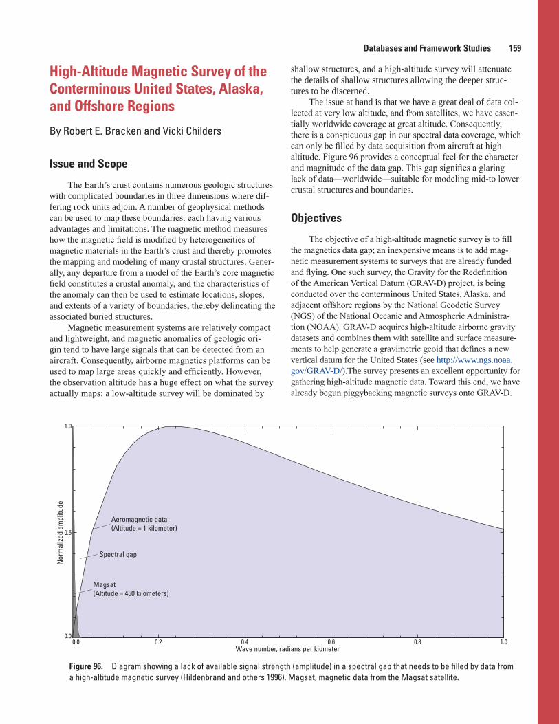
Databases and Framework Studies 159
High-Altitude Magnetic Survey of the Conterminous United States, Alaska, and Offshore Regions
By Robert E. Bracken and Vicki Childers
Issue and Scope
The Earth’s crust contains numerous geologic structures with complicated boundaries in three dimensions where dif-fering rock units adjoin. A number of geophysical methods can be used to map these boundaries, each having various advantages and limitations. The magnetic method measures how the magnetic field is modified by heterogeneities of magnetic materials in the Earth’s crust and thereby promotes the mapping and modeling of many crustal structures. Gener-ally, any departure from a model of the Earth’s core magnetic field constitutes a crustal anomaly, and the characteristics of the anomaly can then be used to estimate locations, slopes, and extents of a variety of boundaries, thereby delineating the associated buried structures.
Magnetic measurement systems are relatively compact and lightweight, and magnetic anomalies of geologic ori-gin tend to have large signals that can be detected from an aircraft. Consequently, airborne magnetics platforms can be used to map large areas quickly and efficiently. However, the observation altitude has a huge effect on what the survey actually maps: a low-altitude survey will be dominated by
shallow structures, and a high-altitude survey will attenuate the details of shallow structures allowing the deeper struc-tures to be discerned.
The issue at hand is that we have a great deal of data col-lected at very low altitude, and from satellites, we have essen-tially worldwide coverage at great altitude. Consequently, there is a conspicuous gap in our spectral data coverage, which can only be filled by data acquisition from aircraft at high altitude. Figure 96 provides a conceptual feel for the character and magnitude of the data gap. This gap signifies a glaring lack of data—worldwide—suitable for modeling mid-to lower crustal structures and boundaries.
Objectives
The objective of a high-altitude magnetic survey is to fill the magnetics data gap; an inexpensive means is to add mag-netic measurement systems to surveys that are already funded and flying. One such survey, the Gravity for the Redefinition of the American Vertical Datum (GRAV-D) project, is being conducted over the conterminous United States, Alaska, and adjacent offshore regions by the National Geodetic Survey (NGS) of the National Oceanic and Atmospheric Administra-tion (NOAA). GRAV-D acquires high-altitude airborne gravity datasets and combines them with satellite and surface measure-ments to help generate a gravimetric geoid that defines a new vertical datum for the United States (see http://www.ngs.noaa.gov/GRAV-D/).The survey presents an excellent opportunity for gathering high-altitude magnetic data. Toward this end, we have already begun piggybacking magnetic surveys onto GRAV-D.
Figure 96. Diagram showing a lack of available signal strength (amplitude) in a spectral gap that needs to be filled by data from a high-altitude magnetic survey (Hildenbrand and others 1996). Magsat, magnetic data from the Magsat satellite.
Nor
mal
ized
ampl
itude
Aeromagnetic data(Altitude = 1 kilometer)
Magsat(Altitude = 450 kilometers)
Spectral gap
Wave number, radians per kiometer0.0
0.0
0.5
1.0
0.2 0.4 0.6 0.8 1.0

160 Developing Integrated Methods to Address Complex Resource and Environmental Issues
Background
Over the years, beginning in the early 1990s, we have developed a solid background and understanding of the rationale, issues, and procedures associated with flying high-altitude surveys. This expertise is described in Hildenbrand and others (1996) when we were working with the ER-2 high-altitude aircraft, and again in Hildenbrand and others (2002) when we were working with a Canberra high-altitude aircraft. Our most recent endeavor, spring of 2011, was a survey pig-gybacked onto a NOAA P-3 aircraft flying in northern Alaska under the GRAV-D project.
Results and Conclusions
The recent P-3 aircraft work has resulted in not only a good high-altitude magnetic dataset in northern Alaska but also a new method for removing aircraft interference from magnetic data collected at high altitude. This work has not yet been published.
In the bigger picture, however, understanding the structure of the mid- to lower crust is essential for develop-ing hazards prediction and mitigation methods, for predicting resource locations and extents, and for generally adding to our knowledge of Earth processes and enhancement of future geosciences research.
Filling the spectral data gap shown in figure 96 by flying a high-altitude magnetic survey of the conterminous United States and Alaska would directly provide much-needed data for improving the North American magnetic anomaly map (NAMAM) to include the accurate intermediate wavelengths required for deep crustal interpretation. The NAMAM (North American Magnetic Anomaly Group, 2002) distills magnetic information gathered by all surveys into what is perhaps the most important single reference used for interpreting continen-tal-scale crustal magnetic signatures of North America. The Australians have produced a similar map, which is now in its fifth generation (http://explorationgeophysics.info/?p=1131), and incorporates a great deal of information from high-altitude data acquisition.
However, the magnetics data gap remains worldwide: few countries, except Australia, have endeavored to conduct systematic magnetic surveys at high altitude.
Collaborators
National Oceanic and Atmospheric Administration, National Geodetic Survey GRAV-D project. Project Manager: Vicki Childers
References Cited
Hildenbrand, T.G., Acuna, Mario, Bracken, R.E., Hardwick, Doug, Hinze, W.J., Keller, G.R., Phillips, J.D., and Roest, W.R., 2002, Rationale and operational plan for a U.S. high-altitude magnetic survey: U.S. Geological Survey Open-File Report 02–366, 22 p., http://pubs.usgs.gov/of/2002/0366/.
Hildenbrand, T.G., Blakely, R.J., Bracken, R.E., Edwards, Lynn, Hardwick, Doug, Hinze, W.J., Labson, Vic, Malliot, Hal, Nabighian, Misac, Nilsson, Bruno, Phillips, Jeff, Quinn, J.M., and Roest, Walter, 1996, Rationale and prelim-inary operational plan for a high-altitude magnetic survey over the United States: U.S. Geological Survey Open-File Report 96–276, 55 p.
North American Magnetic Anomaly Group, 2002, Magnetic Anomaly Map of North America: U.S. Geological Survey Special Map, scale 1:5,000,000, http://pubs.usgs.gov/sm/mag_map/.

Publishing support provided by: Denver Publishing Service Center
For more information concerning this publication, contact:Center Director, USGS Crustal Geophysics and Geochemistry Science CenterBox 25046, Mail Stop 964Denver, CO 80225(303) 236-1312
Or visit the Crustal Geophysics and Geochemistry Science Center Web site at:http://crustal.usgs.gov/
Or visit the Central Energy Resources Science Center Web site at:http://energy.usgs.gov/

Smith and others, eds.—
Developing Integrated M
ethods to Address Com
plex Resource and Environmental Issues—
Circular 1413
ISSN 1067-084X (print)ISSN 2330-5703 (online)http://dx.doi.org/10.3133/cir1413