Embed Size (px)
Citation preview
sac13-0509_fig40_updated
19452010
1966: Grape irrgation ends
1978: Citrus expands
Cumulative storage change
–500
Sealevel
1,000FEET
NorthwestSoutheast
Cumulative storage change
U.S. Department of the InteriorU.S. Geological Survey
Scientific Investigations Report 2015–5150
Prepared in cooperation with the Borrego Water District
Hydrogeology, Hydrologic Effects of Development, and Simulation of Groundwater Flow in the Borrego Valley, San Diego County, California
Basement
Lower aquifer
Middle aquifer
Upper aquifer
2010
Current usage trend—2060
1945
Optimized usage trend—2060
Recreationalpumping
Municipalpumping
Agriculturalpumping
1966: Grape irrigation ends
1978: Citrus expands
1945
2010
Cumulative storage change

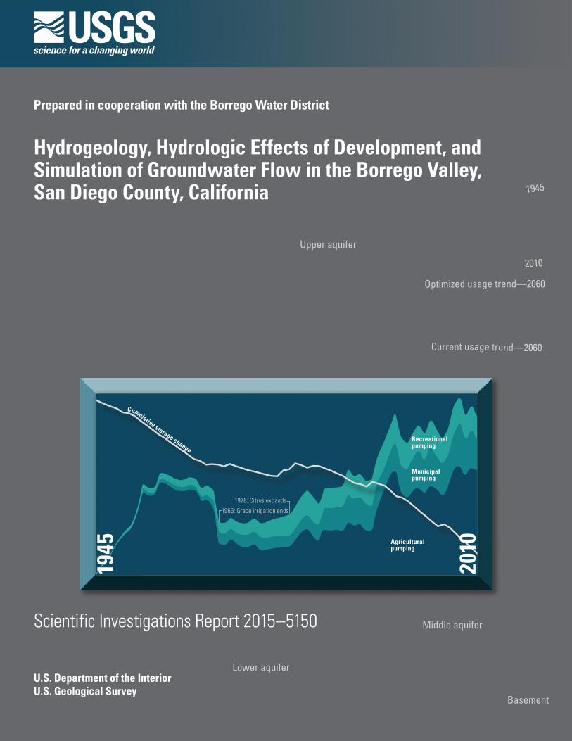
Cover. Background—Cross section showing the simulated groundwater level tables for 1945 and 2010 and for management scenarios projected for 2060, Borrego Valley Hydrologic Model, Borrego Valley, California.
Foreground—Simulated annual groundwater pumpage and climatic patterns from the Borrego Valley Hydrologic Model, Borrego Valley, California, 1945–2010, by water use.
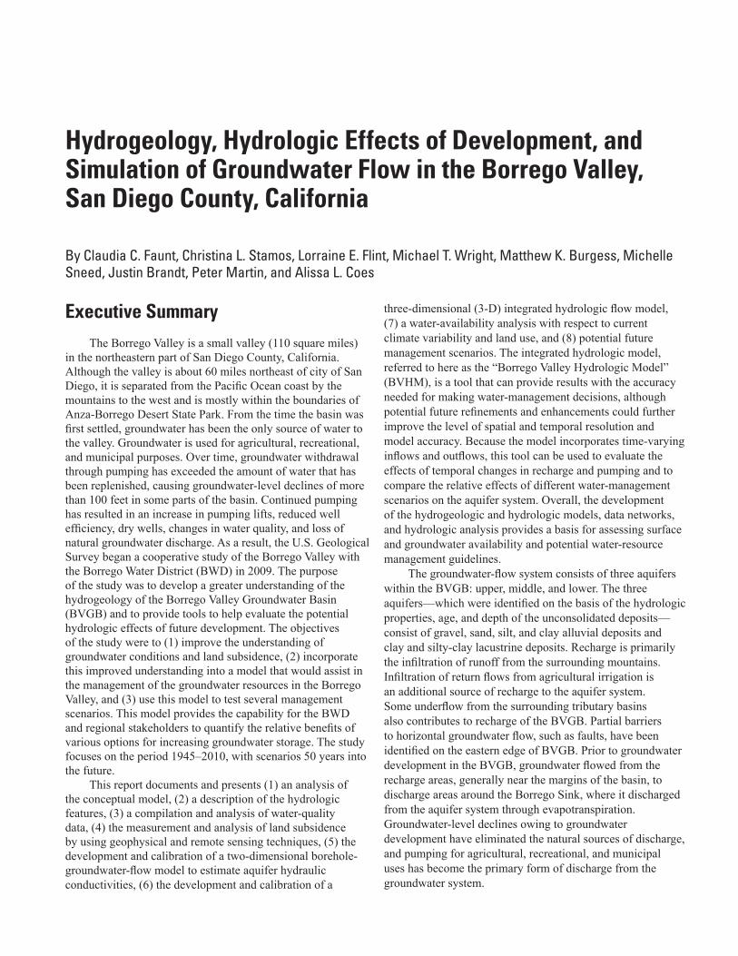
Hydrogeology, Hydrologic Effects of Development, and Simulation of Groundwater Flow in the Borrego Valley, San Diego County, California
By Claudia C. Faunt, Christina L. Stamos, Lorraine E. Flint, Michael T. Wright, Matthew K. Burgess, Michelle Sneed, Justin Brandt, Peter Martin, and Alissa L. Coes
Prepared in cooperation with the Borrego Water District
Scientific Investigations Report 2015–5150
U.S. Department of the InteriorU.S. Geological Survey

U.S. Department of the InteriorSALLY JEWELL, Secretary
U.S. Geological SurveySuzette M. Kimball, Acting Director
U.S. Geological Survey, Reston, Virginia: 2015
For more information on the USGS—the Federal source for science about the Earth, its natural and living resources, natural hazards, and the environment—visit http://www.usgs.gov or call 1–888–ASK–USGS.
For an overview of USGS information products, including maps, imagery, and publications, visit http://www.usgs.gov/pubprod/.
Any use of trade, firm, or product names is for descriptive purposes only and does not imply endorsement by the U.S. Government.
Although this information product, for the most part, is in the public domain, it also may contain copyrighted materials as noted in the text. Permission to reproduce copyrighted items must be secured from the copyright owner.
Suggested citation:Faunt, C.C., Stamos, C.L., Flint, L.E., Wright, M.T., Burgess, M.K., Sneed, Michelle, Brandt, Justin, Martin, Peter, and Coes, A.L., 2015, Hydrogeology, hydrologic effects of development, and simulation of groundwater flow in the Borrego Valley, San Diego County, California: U.S. Geological Survey Scientific Investigations Report 2015–5150, 135 p., http://dx.doi.org/10.3133/sir20155150.
ISSN 2328-0328 (online)

iii
This project could not have been completed without the help of many individuals and organizations. First, the authors acknowledge the Borrego Water District for their support of this study. The work would not have been possible without the data, technical input, and collaboration provided by the Borrego Water District. In particular, Jerry Rolwing provided invaluable assistance. Lyle Brecht, Board Member, Borrego Water/Sewer District, supplied important insight. We are grateful to our U.S. Geological Survey colleagues Larry Schneider, illustrator; Steve Predmore, geographic information system specialist; and the technical reviewers. Finally, a debt of gratitude is owed to the authors of the previous studies done in Borrego Valley.
Acknowledgments
iv
Contents
Executive Summary .......................................................................................................................................1Introduction.....................................................................................................................................................4
Purpose and Scope ..............................................................................................................................7Approach ................................................................................................................................................7Accessing Data .....................................................................................................................................7
Description of Study Area ............................................................................................................................8Previous Studies ............................................................................................................................................8Hydrologic System .........................................................................................................................................9
Climate ....................................................................................................................................................9Potential Evapotranspiration ..............................................................................................................9Climatic Trends ....................................................................................................................................13Land Use ...............................................................................................................................................13
Hydrogeology................................................................................................................................................26Geologic Structures............................................................................................................................26Configuration of Basin .......................................................................................................................26Geologic Units .....................................................................................................................................26Aquifers ................................................................................................................................................31Three-Dimensional Hydrogeologic Framework Model ................................................................36
Selection and Compilation of Existing Well Data .................................................................36Adjustment of Aquifer Surfaces ..............................................................................................36Texture Model .............................................................................................................................37
Classification of Texture from Drillers’ Logs and Regularization of Well Data .......38Geostatistical Model of Coarse-Grained Texture ........................................................38
Groundwater-Flow and Groundwater-Level Change ....................................................................43Groundwater Recharge .....................................................................................................................43
Sources of Recharge ................................................................................................................43Transient Estimates of Natural Recharge from the Basin Characterization Model .......48
Groundwater Discharge ....................................................................................................................51Evapotranspiration ....................................................................................................................55Underflow Out of the Basin ......................................................................................................55Groundwater Pumping ..............................................................................................................55
Agricultural Water Use ....................................................................................................56Recreational Water Use ..................................................................................................56Municipal Water Use .......................................................................................................56
Groundwater-Quality Sampling and Wellbore Flow...............................................................................60Wellbore Flow and Depth-Dependent Water-Quality Sampling .................................................61Sources of Water-Quality Data.........................................................................................................61
Groundwater Quality and Age ...................................................................................................................63Changes in Groundwater Quality Compared to Changes in Groundwater Levels ...................63Distribution and Variation of Groundwater Quality .......................................................................65
Distribution of Nitrates and Total Dissolved Solids ..............................................................65Variations in Water Quality with Depth ..................................................................................65
Groundwater Age................................................................................................................................68
v
Land Subsidence..........................................................................................................................................70Global Positioning System ................................................................................................................70
Ellipsoid Heights and Elevations .............................................................................................70Land Subsidence at Geodetic Monuments ...........................................................................73GPS Derived Elevations ............................................................................................................73
Interferometric Synthetic Aperture Radar ....................................................................................73Groundwater-Flow Models ........................................................................................................................77
Wellbore-Groundwater-Flow Model................................................................................................77Integrated Hydrologic Model ............................................................................................................77
Discretization and Boundaries ................................................................................................79Spatial Discretization .......................................................................................................79Temporal Discretization ...................................................................................................79
Initial Conditions ........................................................................................................................82Aquifer Type ................................................................................................................................82Aquifer Characteristics .............................................................................................................83
Textural Analysis ...............................................................................................................83Calculation of Hydraulic Properties ...............................................................................83Hydraulic Conductivity of Lithologic End Members ....................................................85Storage Properties ...........................................................................................................86Unsaturated Hydraulic Properties .................................................................................86
Recharge .....................................................................................................................................88Water-Balance Subregions .....................................................................................................90Landscape Water Use ...............................................................................................................90
Delivery Requirement .......................................................................................................92Soils ................................................................................................................................92Land Use .............................................................................................................................92
Discharge ....................................................................................................................................92Natural Discharge ............................................................................................................92Groundwater Pumpage ....................................................................................................92
Agricultural Pumpage ............................................................................................97Recreational Pumpage ...........................................................................................97Municipal Pumpage ................................................................................................97
Groundwater Inflows and Outflows ........................................................................................97Specified (No Flow) Flow Boundaries ...........................................................................97Specified Flow Boundaries .............................................................................................99Specified (Constant) Head Boundary ............................................................................99
Model Calibration................................................................................................................................99Parameter Data ..........................................................................................................................99Observation Data .....................................................................................................................103Regularization ...........................................................................................................................106
Pumpage Observations ..................................................................................................107Groundwater-Level Maps ..............................................................................................108
Calibration Procedure .............................................................................................................108
Contents—Continued
vi
Farm Process Parameters .............................................................................................108Hydraulic Parameters ....................................................................................................112Streamflow Properties ...................................................................................................112
Sensitivity Analysis ...........................................................................................................................112Model Uncertainty, Limitations, and Improvements ..................................................................113
Hydrologic Flow Analysis ........................................................................................................................115Future Groundwater-Management Scenarios ......................................................................................122
Scenario 1: Status Quo ....................................................................................................................124Scenarios 2–4: Low, Medium, and High Municipal Growth Over 50 Years .............................124Scenario 5: Water-Usage Reduction to Avoid Future Groundwater Storage
Depletion Over 50 Years .....................................................................................................124Scenario 6: Management Scenario for Rapid Changes Over 20 Years ...................................124
Summary and Conclusions .......................................................................................................................127References Cited........................................................................................................................................130
Contents—Continued
Figures
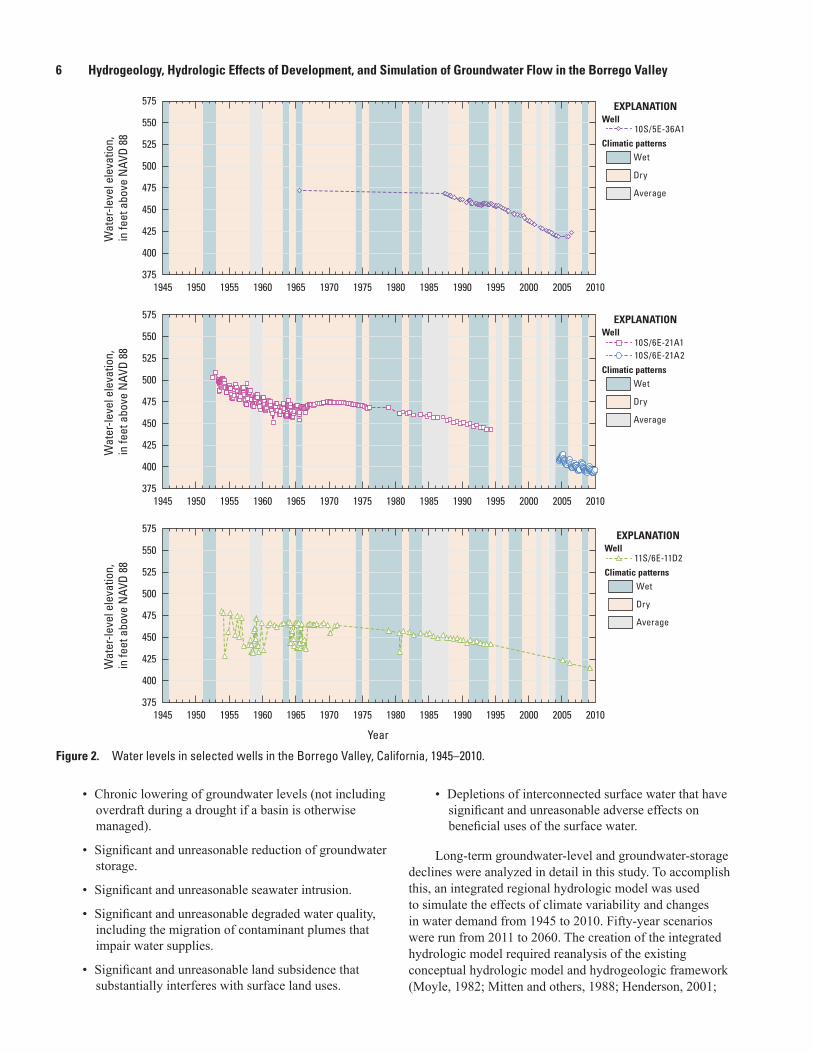
1. Map showing location of the Borrego Valley, California .......................................................5 2. Graphs showing water levels in selected wells in the Borrego Valley,
California, 1945–2010 ....................................................................................................................6 3. Graphs showing A, average annual precipitation and B, cumulative departure
of precipitation for Borrego Valley, California .......................................................................10 4. Maps showing estimated average annual for Borrego Valley, California,
1945–2010, of A, precipitation and B, potential evapotranspiration ...................................11 5. Graphs showing trends in climate for the Borrego Valley, California, 1899–2008,
including A, estimated minimum and maximum annual mean air temperatures; B, annual precipitation; and C, estimated potential evapotranspiration, Borrego Valley .............................................................................................................................14
6. Maps showing land use in the Borrego Valley, California, during A, pre-development; B, 1953; C, 1954; D, 1959; E, 1968; F, 1979; G, 1980; H, 1992; I, 1995; J, 2000; and K, 2009 ........................................................................................................15
7. Maps showing Borrego Valley, California, showing A, geology; B, hydrogeology; and C, generalized hydrogeologic cross sections A-A’ and B-B’ .......................................27
8. Map showing gridded depth from land surface to basement rock in the Borrego Valley, California ..........................................................................................................30
9. Map showing location of wells with driller’s and (or) geophysical logs used to develop the hydrogeologic framework model for the Borrego Valley, California ............32
10. Maps showing extent and approximate thickness of aquifers in Borrego Valley, California, A, upper; B, middle; and C, lower ..........................................................................33
11. Generalized cross sections of Borrego Valley, California: A, northwest to southeast, modified from Moyle (1982), and B, southwest to northeast, drawn by using data from geophysical logs collected in 2012 ...........................................37
12. Maps showing percentage of coarse-grained deposits in aquifers of Borrego Valley, California: A, upper; B, middle; and C, lower ..........................................................................40
vii
13. Maps showing water-level elevations and direction of groundwater flow in Borrego Valley, California, for A, 1945, approximately predevelopment, and B, 2010 ....................44
14. Graphs showing water-level elevations in selected wells in parts of the Borrego Valley, California, 1950–2010: A, northern; B, west–northern; C, middle; and D, southern ........................................................................................................46
15. Graphs showing discharge of creeks in Borrego Valley, California, 1950–2004: A, Coyote Creek; B, Borrego Palm Creek; and C, San Felipe Creek ...................................47
16. Map showing drainage basin boundaries and geology used in the Basin Characterization Model to estimate climate-driven natural recharge in the Borrego Valley, California ..........................................................................................................49
17. Graph showing measured annual streamflow at Borrego Palm Creek streamgage and simulated annual streamflow from the Basin Characterization Model for the Borrego Palm Creek drainage watershed, Borrego Valley, California ..........................................................................................................50
18. Maps showing spatially distributed values for the Borrego Valley, California, 1971–2000, of potential A, runoff and B, recharge ................................................................52
19. Graphs showing simulated values for the Borrego Valley, California, 1940–2007, of total annual A, potential runoff into the valley; B, potential recharge in upstream portions of the watershed (potential underflow); and C, recharge (underflow and runoff) into the valley .....................................................................................54
20. Graph showing annual and cumulative total pumpage, Borrego Valley, California, 1945–2000 ..................................................................................................................55
21. Graph showing annual and cumulative municipal pumpage, Borrego Valley, California, 1945–2010 ..................................................................................................................59
22. Graph showing average percentage of reported annual pumpage, by month, for Borrego Water District wells, Borrego Valley, California, 1997–2010 ..........................59
23. Graph showing pumpage by Rams Hill Development and total pumpage by Borrego Water District, Borrego Valley, California, 1983–2010 ...........................................60
24. Well construction for well 10S/6E-35Q1, Borrego Valley, California: A, wellbore-flow log and B, concentrations of selected dissolved constituents by depth, under pumping conditions .......................................................................................62
25. Graphs showing concentrations of total dissolved solids and sulfate, and groundwater levels for wells A, 10S/6E-18R1, B, 11S/6E-7K3, and C, 11S/6E-23J1 in the Borrego Valley, California, 1980–2010 ..........................................................................64
26. Map showing distribution of nitrate as nitrogen concentrations in the upper, middle, and lower aquifers, Borrego Valley, California, for the most recent sample ......66
27. Map showing distribution of total dissolved solids concentrations in the upper, middle, and lower aquifers, Borrego Valley, California ........................................................67
28. Map showing distribution of tritium values and uncorrected carbon-14 ages for wells in the Borrego Valley, California ....................................................................................69
29. Map showing location of geodetic monuments used as Global Positioning System stations, Borrego Valley, California ...........................................................................71
30. Graph showing vertical position of Continuous Global Positioning System site P486, 2005–10, in the Borrego Valley, California ....................................................................74
31. Map showing line and area of equal subsidence as interpreted from Interferometric Synthetic Aperture Radar satellite imagery of the Borrego Valley, California, November 2003–September 2007 .............................................................................................76
Figures—Continued
viii
32. Diagram showing simulated lithology, calibrated hydraulic conductivity distribution, and simulated and measured flow logs from well 10S/6E-35Q1, Borrego Valley, California ..........................................................................................................78
33. Map showing model grid with active model cells for the upper and lower aquifers in the Borrego Valley Hydrologic Model, Borrego Valley, California .................81
34. Graph showing model grid with geologic types of depositional zones used for parameter zones of hydraulic properties for the Borrego Valley Hydrologic Model, Borrego Valley, California ............................................................................................84
35. Schematic diagram showing magnitudes of specific yield for the upper, middle, and lower aquifers, Borrego Valley, California ......................................................................86
36. Map showing model grid with texture zones used to define the distribution of specific yield for the Borrego Valley Hydrologic Model, Borrego Valley, California .......87
37. Map showing model-grid stream cells used to simulate streamflow in the Borrego Valley Hydrologic Model, Borrego Valley, California ............................................89
38. Map showing model grid with water balance subregions used to account for water usage in the Borrego Valley, California .......................................................................91
39. Map showing model grid with two types of soil categories used in the Borrego Valley Hydrologic Model, Borrego Valley, California ............................................................96
40. Graphs showing simulated annual groundwater pumpage and climatic patterns from the Borrego Valley Hydrologic Model, Borrego Valley, California, 1945–2010, by A, aquifer and B, water use .............................................................................98
41. Map showing location of observation wells used in the calibration of the Borrego Valley Hydrologic Model, Borrego Valley, California ..........................................104
42. Hydrographs showing simulated and measured water-level elevations for the Borrego Valley Hydrologic Model, Borrego Valley, California, 1945–2010 ......................105
43. Histogram of distribution of groundwater-level residual (observed minus simulated) values for the Borrego Valley Hydrologic Model, Borrego Valley, California ....................................................................................................................................107
44. Graph showing simulated water level-elevations in relation to measured water-level elevations for the Borrego Valley Hydrologic Model, California, Borrego Valley, California ........................................................................................................107
45. Maps showing simulated water levels for the Borrego Valley Hydrologic Model, Borrego Valley, California, A, in 1945; B, 2010; and C, simulated drawdown from 1945 to 2010 ..................................................................................................109
46. Graph showing most sensitive parameters for the Borrego Valley Hydrologic Model, Borrego Valley, California ..........................................................................................113
47. Graphs showing simulated components of the basic groundwater budget by using climatic patterns A, with no anthropogenic effects and B, with anthropogenic effects for the Borrego Valley Hydrologic Model, Borrego Valley, California, 1945–2010 ...................................................................................................116
48. Graphs showing simulated components of the net groundwater budget from the Borrego Valley Hydrologic Model, Borrego Valley, California, 1945–2010, by using climatic patterns A, with no anthropogenic effects and B, with anthropogenic effects ..............................................................................................................117
49. Graph showing precipitation, streamflow, and underflow from adjacent watersheds and basins for the Borrego Valley, California, 1945–2010 ............................118
Figures—Continued
ix
50. Graphs showing simulated landscape budget with climatic patterns from the Borrego Valley Hydrologic Model, Borrego Valley, California, 1945–2010, A, with no anthropogenic effects and B, with anthropogenic effects ..........................................119
51. Graph showing simulated monthly net groundwater budget, Borrego Valley Hydrologic Model, Borrego Valley, California, 2010 ............................................................121
52. Graph showing simulated annual and cumulative changes in groundwater storage by using climatic patterns with no anthropogenic effects and with anthropogenic effects, Borrego Valley Hydrologic Model, Borrego Valley, California, 1945–2010 ................................................................................................................121
53. Graph showing cumulative change in groundwater storage for six water-management scenarios simulated by using the Borrego Valley Hydrologic Model, Borrego Valley, California, 1945–2060 .................................................123
54. Cross section showing the simulated groundwater level tables for 1945 and 2010 and for six management scenarios projected for 2060, Borrego Valley Hydrologic Model, Borrego Valley, California ......................................................................123
55. Map showing simulated drawdown projected for scenario 1, or the status quo scenario, 2060 minus 2010, Borrego Valley Hydrologic model, Borrego Valley, California ....................................................................................................................................125
56. Map showing simulated drawdown projected for Scenario 6, 2060 minus 2010, Borrego Valley Hydrologic Model, Borrego Valley, California ..........................................126
Figures—Continued
Tables
1. Mean and standard deviation of estimated annual air temperature, precipitation, and potential evapotranspiration for three periods during 1899–2008 obtained by using the Parameter-Elevation Regressions on Independent Slopes Model database for the regional Borrego Valley drainage basin, California .........................................................................................................................13
2. Description of aquifers, Borrego Valley, California ...............................................................36 3. Textures used to describe lithology recorded on drillers’ logs, Borrego Valley,
California ......................................................................................................................................38 4. Input for geostatistical model, Borrego Valley, California ...................................................39 5. Estimated and reported total municipal pumpage, Borrego Valley, California,
1945–2010 .....................................................................................................................................57 6. Location of geodetic monuments in the land-subsidence monitoring network
with ellipsoid heights for 2009, and elevations for 1969, 1978, 1995, and 2009, Borrego Valley, California ..........................................................................................................72
7. Interferograms processed from the European Space Agency’s satellites for Borrego Valley, California ..........................................................................................................75
8. Details of radial groundwater-flow model construction for well 10S/6E-35Q1, Borrego Valley, California ..........................................................................................................78
9. Summary of One Water Hydrologic Model packages and processes used in the integrated hydrologic model of Borrego Valley, California ..................................................80
10. Summary of groupings of water-balance subregions into regions for the Borrego Valley Hydrologic Model, Borrego Valley, California ............................................82
x
11. Coordinates of the Borrego Valley Hydrologic Model for Borrego Valley, California .....82 12. Summary of hydraulic properties from previous studies and the radial
groundwater-flow model, Borrego Valley, California ...........................................................85 13. Summary of Borrego Valley land-use types in the Borrego Valley Hydrologic
Model, Borrego Valley, California ............................................................................................93 14. Monthly crop coefficients for each land-use type simulated in the Borrego
Valley Hydrologic Model, Borrego Valley, California ............................................................93 15. Summary of fractions of transpiration and evaporation, by month, for Borrego
Valley land-use type, or virtual crops, Borrego Valley, California ......................................94 16. Monthly efficiency for each land-use type, or virtual crop, simulated in the
Borrego Valley Hydrologic Model, Borrego Valley, California ............................................95 17. Percentage of each land-use type, or virtual crop, used in simulations for
11 periods of mapped land use, Borrego Valley, California .................................................95 18. Parameter values estimated for the Borrego Valley Hydrologic Model, Borrego
Valley, California .......................................................................................................................100 19. Simplified groundwater budget for pre-development and 2010, Borrego Valley
Hydrologic Model, Borrego Valley, California ......................................................................118 20. Groundwater budgets for six management scenarios from the Borrego Valley
Hydrologic Model, Borrego Valley, California, 2011–60 .....................................................122
Tables—Continued
xi
14C carbon-142-D two-dimensional3-D three-dimensionalasl above sea levelBAR Borrego Air RanchBCM Basin Characterization Modelbls below land surfaceBSPCSD Borrego Springs Park and Community Service DistrictBVGB Borrego Valley Groundwater BasinBVHM Borrego Valley Hydrologic ModelBWD Borrego Water DistrictCA-DPH California Department of Public HealthCA-DWR California Department of Water ResourcesCA-MCL California maximum contaminant levelCA-SMCL California secondary maximum contaminant levelCGPS Continuous Global Positioning SystemCIR crop irrigation requirementEM electromagneticERS Earth Remote SensingET evapotranspirationETo evapotranspiration rateFHB1 Flow Head BoundaryFMP Farm ProcessGIS Geographic Information SystemGPS global positioning systemInSAR Interferometric Synthetic Aperture RadarK hydraulic conductivityKC crop coefficientsMF2K5 MODFLOW-2005MNW2 multi-mode wellsMODIS Moderate-Resolution Imaging SpectroradiometerNO3-N nitrate as nitrogenNWIS National Water Information SystemNWISWeb USGS National Water Information System Web pageOWHM One Water Hydrologic ModelPEST parameter estimation softwarePET potential evapotranspirationPRISM Parameter-Elevation Regressions on Independent Slopes ModelQya older and younger alluviumRTK real time kinematicSAR Synthetic Aperture RadarSFR Streamflow Routing PackageSGMA Sustainable Groundwater Management ActSOPAC Scripps Orbit and Permanent Array CenterSTATSGO State Soil Geographic DatabaseTDS total dissolved solidsTFDR total farm delivery requirementTU tritium unitsUPW Upstream Weighting PackageUSGS U.S. Geological SurveyUZF unsaturated-zone modelWBS water-balance subregionsybp years before present
Abbreviations
xii
Inch/Pound to International System of Units
Multiply By To obtain
Lengthinch (in.) 25.4 millimeter (mm)inch (in.) 25,400 micrometer (µm)foot (ft) 0.3048 meter (m)mile (mi) 1.609 kilometer (km)
Areasquare mile (mi2) 2.590 square kilometer (km2)
Volumeounce, fluid (fl. oz) 29.5735 milliliter (mL)gallon (gal) 3.785 liter (L) acre-foot (acre-ft) 1,233 cubic meter (m3)
Flow rateacre-foot per year (acre-ft/yr) 1,233 cubic meter per year (m3/yr)foot per day (ft/d) 0.3048 meter per day (m/d)foot per year (ft/yr) 0.3048 meter per year (m/yr)gallon per minute (gal/min) 0.06309 liter per second (L/s)gallon per day (gal/d) 0.003785 cubic meter per day (m3/d)inch per year (in/yr) 25.4 millimeter per year (mm/yr)cubic foot per month (ft3/mo) 0.0009 cubic meter per day (m3/d)
Specific capacitygallon per minute per foot [(gal/min)/ft)] 0.2070 liter per second per meter [(L/s)/m]
Hydraulic conductivityfoot per day (ft/d) 0.3048 meter per day (m/d)
Temperature in degrees Celsius (°C) may be converted to degrees Fahrenheit (°F) as °F = (1.8 × °C) + 32.
Datum
Vertical coordinate information is referenced to the North American Vertical Datum of 1988 (NAVD 88).
Horizontal coordinate information is referenced to the North American Datum of 1983 (NAD 83).
Elevation, as used in this report, refers to distance above the vertical datum.
Supplemental Information
Transmissivity: The standard unit for transmissivity is cubic foot per day per square foot times foot of aquifer thickness [(ft3/d)/ft2]ft. In this report, the mathematically reduced form, foot squared per day (ft2/d), is used for convenience.
Specific conductance is given in microsiemens per centimeter at 25 degrees Celsius (µS/cm at 25 °C).
Concentrations of chemical constituents in water are given in either milligrams per liter (mg/L) or micrograms per liter (µg/L).
Conversion Factors

xiii
This page intentionally left blank.

xiv
This page intentionally left blank.
Hydrogeology, Hydrologic Effects of Development, and Simulation of Groundwater Flow in the Borrego Valley, San Diego County, California
By Claudia C. Faunt, Christina L. Stamos, Lorraine E. Flint, Michael T. Wright, Matthew K. Burgess, Michelle Sneed, Justin Brandt, Peter Martin, and Alissa L. Coes
Executive SummaryThe Borrego Valley is a small valley (110 square miles)
in the northeastern part of San Diego County, California. Although the valley is about 60 miles northeast of city of San Diego, it is separated from the Pacific Ocean coast by the mountains to the west and is mostly within the boundaries of Anza-Borrego Desert State Park. From the time the basin was first settled, groundwater has been the only source of water to the valley. Groundwater is used for agricultural, recreational, and municipal purposes. Over time, groundwater withdrawal through pumping has exceeded the amount of water that has been replenished, causing groundwater-level declines of more than 100 feet in some parts of the basin. Continued pumping has resulted in an increase in pumping lifts, reduced well efficiency, dry wells, changes in water quality, and loss of natural groundwater discharge. As a result, the U.S. Geological Survey began a cooperative study of the Borrego Valley with the Borrego Water District (BWD) in 2009. The purpose of the study was to develop a greater understanding of the hydrogeology of the Borrego Valley Groundwater Basin (BVGB) and to provide tools to help evaluate the potential hydrologic effects of future development. The objectives of the study were to (1) improve the understanding of groundwater conditions and land subsidence, (2) incorporate this improved understanding into a model that would assist in the management of the groundwater resources in the Borrego Valley, and (3) use this model to test several management scenarios. This model provides the capability for the BWD and regional stakeholders to quantify the relative benefits of various options for increasing groundwater storage. The study focuses on the period 1945–2010, with scenarios 50 years into the future.
This report documents and presents (1) an analysis of the conceptual model, (2) a description of the hydrologic features, (3) a compilation and analysis of water-quality data, (4) the measurement and analysis of land subsidence by using geophysical and remote sensing techniques, (5) the development and calibration of a two-dimensional borehole-groundwater-flow model to estimate aquifer hydraulic conductivities, (6) the development and calibration of a
three-dimensional (3-D) integrated hydrologic flow model, (7) a water-availability analysis with respect to current climate variability and land use, and (8) potential future management scenarios. The integrated hydrologic model, referred to here as the “Borrego Valley Hydrologic Model” (BVHM), is a tool that can provide results with the accuracy needed for making water-management decisions, although potential future refinements and enhancements could further improve the level of spatial and temporal resolution and model accuracy. Because the model incorporates time-varying inflows and outflows, this tool can be used to evaluate the effects of temporal changes in recharge and pumping and to compare the relative effects of different water-management scenarios on the aquifer system. Overall, the development of the hydrogeologic and hydrologic models, data networks, and hydrologic analysis provides a basis for assessing surface and groundwater availability and potential water-resource management guidelines.
The groundwater-flow system consists of three aquifers within the BVGB: upper, middle, and lower. The three aquifers—which were identified on the basis of the hydrologic properties, age, and depth of the unconsolidated deposits—consist of gravel, sand, silt, and clay alluvial deposits and clay and silty-clay lacustrine deposits. Recharge is primarily the infiltration of runoff from the surrounding mountains. Infiltration of return flows from agricultural irrigation is an additional source of recharge to the aquifer system. Some underflow from the surrounding tributary basins also contributes to recharge of the BVGB. Partial barriers to horizontal groundwater flow, such as faults, have been identified on the eastern edge of BVGB. Prior to groundwater development in the BVGB, groundwater flowed from the recharge areas, generally near the margins of the basin, to discharge areas around the Borrego Sink, where it discharged from the aquifer system through evapotranspiration. Groundwater-level declines owing to groundwater development have eliminated the natural sources of discharge, and pumping for agricultural, recreational, and municipal uses has become the primary form of discharge from the groundwater system.
2 Hydrogeology, Hydrologic Effects of Development, and Simulation of Groundwater Flow in the Borrego Valley
The quality of groundwater in the Borrego Valley is a concern because of reliance on groundwater for agricultural, recreational, and municipal supply. Groundwater quality can be affected by land-use activities occurring at or near land surface. These activities include irrigation of vegetated landscapes and the use of septic systems to dispose of wastewater. Groundwater quality can also be affected by declining groundwater levels, because there is the potential for a change in the distribution of flow from underlying aquifers to wells. Historical and current groundwater-quality data were used to determine which constituents were present in relatively high concentrations compared to State water-quality thresholds and whether these constituent concentrations had changed in response to declining groundwater levels. Age-dating isotopes (tritium and carbon-14 [14C]) were analyzed to determine whether modern (tritium-containing) groundwater recharge is occurring in Borrego Valley. Major findings of the groundwater-quality part of this study follow.
• Historical water-quality data show that, in the upper aquifer, total dissolved solids (TDS) and nitrate (as N) exceeded their water-quality thresholds of 500 mg/L (secondary recommended California maximum contaminant level) and 10 mg/L, respectively. At the time of publication, the source of this nitrate is unknown.
• TDS and sulfate are the only constituents that show increasing concentrations with simultaneous declines in groundwater levels.
• TDS and nitrate concentrations were generally highest in the upper aquifer and in the northern part of the Borrego Valley where agricultural activities are primarily concentrated.
• Age-dating isotopes indicate that little natural groundwater recharge is occurring under current (1900–2000) climatic conditions and that almost all of the natural recharge is occurring adjacent to the mountain fronts.
The long-term extraction of groundwater causes increases in the effective or intergranular stresses in the aquifer-system materials; this increased stress can result in irreversible compaction of the aquifer system. This compaction results in land subsidence in many areas where long-term pumping, typically in excess of recharge, has depleted groundwater storage. Three methods were employed as part of this study to assess the land subsidence in Borrego Valley: Global Positioning System (GPS) surveys, continuous GPS (CGPS) data collection, and interferometric synthetic aperture radar (InSAR) remote sensing techniques. InSAR results, derived from synthetic-aperture radar data, provide spatially detailed ground deformation maps (interferograms) that can elucidate spatially detailed patterns of vertical deformation for specific time spans. The InSAR methods complement the GPS surveys and CGPS data, which provide time-series data at a series of
points. The GPS surveys, CGPS data, and InSAR analyses show little land subsidence has occurred in the Borrego Valley (much less than 1 inch in the last 50 years, 1961–2010). Hence, land subsidence attributed to aquifer-system compaction is not currently a problem in the Borrego Valley and is unlikely to be a significant problem in the future.
The GPS surveys were also used to improve the previous crude determinations of elevations for groundwater wells, which were derived from topographic maps and from which groundwater levels and groundwater-level gradients were determined. Historical land-surface elevations were updated for 79 groundwater wells. Historical elevations were changed by more than 5 feet at 10 wells and by almost 30 feet at 1 well. The updated elevations give a better estimate of spatially distributed groundwater levels, particularly the locations of highs and lows of the groundwater table.
The BVHM was developed on the basis of historical conditions (66 years) for the analysis of the use and movement of groundwater and surface water throughout the valley and to provide a basis for addressing groundwater availability and sustainability analyses. The model has a uniform horizontal discretization of 92 acres per cell (2,000 ft by 2,000 ft) and is oriented subparallel to the tectonic structure and to Coyote Creek. Vertically, the model has three layers representing the upper, middle, and lower aquifers. The model was calibrated by using groundwater-level measurements for 1945–2010 and simulates conditions during that period. Natural and anthropogenic recharge and discharge, and the transient nature of these stresses, were simulated.
The main sources of recharge to the system are runoff from creeks and streams draining the surrounding watershed, which quickly seeps into the permeable streambeds and infiltrates through the unsaturated zone, and groundwater underflow from the adjacent basins. Exceptionally large and infrequent storms typically contribute the most water to recharge. Excess flow sometimes terminates in middle of the valley at the Borrego Sink or flows out the southeastern end of the valley along San Felipe Wash. Over the 66-year study period, on average, the natural recharge that reached the saturated groundwater system was approximately 5,700 acre-feet per year (acre-ft/yr), but natural recharge fluctuated in the arid climate from less than 1,000 to more than 25,000 acre-ft/yr. On average, of the 5,700 acre-ft/yr, about 1,700 acre-ft/yr seeps into the ground during wet years and rapidly discharges as evapotranspiration. In addition, approximately 1,400 acre-ft/yr enters the basin as underflow from adjacent basins. Since agricultural, recreational, and municipal land uses have been developed, a relatively small amount of recharge also occurs from excess irrigation water and septic-tank effluent. Recharge from irrigation return flows, as indicated by the model results, was about 10–30 percent of agricultural and recreational pumpages. Although a small amount of recharge from septic systems occurs and can be important locally, it is negligible relative to natural recharge and return flow from agricultural and recreational pumpages.
Executive Summary 3
The BVHM uses a one-dimensional unsaturated-zone model to estimate the delay associated with return flow moving through the unsaturated zone. Depending on the thickness, permeability, and residual moisture content in the relatively thick unsaturated zone, it takes tens to hundreds of years for the bulk of return flow to reach the water table. In addition, not all water that reaches the root zone reaches the water table because some water is lost through evapotranspiration or goes into storage in the unsaturated zone. Therefore, in many areas, water that is applied to previously unirrigated land arrives at the underlying water table decades or longer after it is applied.
Groundwater discharge occurs in three primary forms: (1) evapotranspiration from the ground and through the direct uptake of plants (mostly in and around the Borrego Sink); (2) a small amount of seepage from the southern end of the basin; and (3) groundwater pumping for agricultural, recreational, and municipal uses. Natural discharge from evapotranspiration ranges from approximately 6,500 acre-ft/yr prior to development to virtually zero in the last several decades (1990–2010), because the groundwater levels in the basin dropped below the reach of the mesquite in the basin. Underflow out the southern end of the basin was small and relatively stable over time, at about 500 acre-ft/yr. Groundwater pumpage for agriculture and recreation was estimated on the basis of irrigated acreage and consumptive-use data. Values of pumpage for municipal supply were compiled from water-use records. Estimated combined annual agricultural, recreational, and municipal pumpage peaked at around 19,600 acre-ft from 2005 to 2010.
Results of the calibrated model simulations indicated that simulated groundwater pumpage exceeded simulated actual natural recharge in most years, resulting in an estimated cumulative depletion of groundwater storage of about 450,000 acre-ft from 1945 to 2010. Groundwater pumping resulted in simulated groundwater-level declines of more than 150 ft from 1945 conditions in much of the northern portion of the study area. The decline in groundwater levels was the result of this depletion of groundwater storage. In turn, the simulated decline in groundwater levels resulted in the elimination of almost all of natural discharge through evapotranspiration from the groundwater basin. Because there are few fine-grained, compressible deposits in the aquifer system materials, little aquifer-system compaction and land subsidence have occurred.
The calibrated BVHM was used to simulate the response of the aquifer system to six future 50-year (2011 to 2060) pumping scenarios: (1) no change in the agricultural, recreational, and municipal pumpage rates (status quo); (2–4) various levels of reductions in agricultural and recreational pumpage rates, coupled with low to high increases in municipal pumping rates; (5) reduction of all groundwater pumpage to that needed to avoid future groundwater-storage depletion over 50 years; and (6) a less severe, but more rapid, reduction in all groundwater usage over 20 years, followed by 30 years at a constant much lower pumpage rate.
Results from Scenario 1 (continuation of current, 2010, annual pumpage) indicated that the drawdown observed since pre-development would continue, with a total depletion in groundwater storage of about 1,000,000 acre-ft by 2060. Consequently, the water table declines to the middle aquifer in some areas. Because of the lower hydraulic conductivity and storage properties of the middle aquifer relative to the upper aquifer, continued pumping at these rates would result in larger, more rapid groundwater-level declines in the future and possibly a reduction in groundwater quality. As a result, more or deeper wells could be needed to accomplish similar pumpage rates. Scenarios 2–4 represent combinations of changes in agricultural and recreational pumpages, as well as in municipal pumpage. Although less than Scenario 1 (status quo) pumpage rates, pumpage rates in two of these three scenarios exceed the average annual recharge rate, groundwater levels continue to decline, and there is continued cumulative depletion of groundwater storage. Because more water is being extracted from the groundwater basin than is being recharged either through natural or induced means, groundwater levels continue to decline. As the groundwater table is lowered from the relatively storage-rich and permeable upper aquifer to the middle and lower aquifers, the rate and areal extent at which groundwater levels decline accelerate, and the areal extent over which storage changes would be affected would be larger in the middle and lower aquifers with lower storativities. Furthermore, if the groundwater quality is less desirable deeper in the system, as existing information indicates, then the water quality of groundwater pumpage would deteriorate as deeper sources of water contribute more water to supply wells; this water could require more advanced water treatment than is used at present (2010) for municipal, and potentially, irrigation supply.
The location of the largest drawdown varies with the relative contributions of the three water-use categories (agricultural, recreational, and municipal) to overall pumpage in each scenario. In Scenario 5, water use is reduced in all three categories (agricultural, recreational, and municipal) to reach a sustainable level over a 50-year time span. The California Sustainable Groundwater Management Act (SGMA) of 2014 requires basins to reach sustainable yield. Scenario 5, with its 50-year time span, covers a longer period than is required by the act. The sustainable level for the Borrego Valley, assuming no significant degradation in groundwater quality, equates to total discharge equaling the long-term average recharge to the basin. As human activities change the system, the components of the water budget (inflows, outflows, and changes in storage) also change and must be accounted for in any management decision. Because there currently is little effect on captured recharge or discharge, in this system, ‘sustainability’ is a maximum amount of discharge to avoid future groundwater-storage depletion and is being simplified and equated to this average recharge. As the rate of total groundwater extraction approaches the rate of recharge (meaning all inflows—natural
4 Hydrogeology, Hydrologic Effects of Development, and Simulation of Groundwater Flow in the Borrego Valley
and anthropogenic recharge, including induced recharge from captured water sources) to the aquifer system, the change in groundwater storage, and thus the rate of groundwater storage depletion, approaches zero, indicating no additional loss in storage. In the long run, the average change in groundwater storage would be negligible when the basin is operated at the sustainable level; however, groundwater levels and storage changes would fluctuate as they have historically with climatic variability. For example, during relatively wet years, more water could go into storage than is extracted. In turn, during moderate and relatively dry years, more water would be extracted than goes into storage.
In order to simulate a realistic approach for meeting SGMA requirements on the 20-year SGMA timeline for implementation, in Scenario 6, municipal and recreational pumpages both were reduced to 50 percent of current (2010) rates, and agricultural pumpage was reduced to 40 percent of current rates. These reductions were applied linearly over 20 years and continued for the next 30 years until 2060. With these reductions, at 2060, recharge approximates discharge. Simulated drawdowns are approximately 50 feet over a broad part of the basin. Drawdown and groundwater-storage losses continue in areas where agricultural, recreational, and municipal pumping occurs. In the long run, groundwater levels would stabilize and would not decline as they would for the Scenario 1 simulation, which had continued significant groundwater level and storage declines. However, changes in groundwater storage would fluctuate with climatic variability. Because climate models indicated greater variability in natural recharge in the future than during historical periods, the variability of groundwater-storage changes could also increase. Managed artificial recharge through engineered, enhanced infiltration of storm water or imported surface water is a water-management strategy that could help alleviate the demands on the valley’s groundwater system.
IntroductionThe Borrego Valley is a small valley in the northeastern
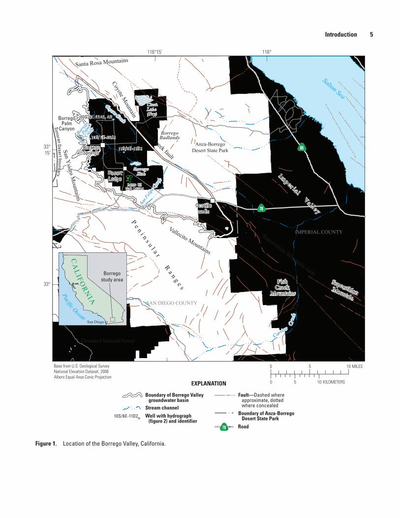
part of San Diego County, California, about 60 miles northeast of San Diego (fig. 1). Native Americans inhabited the valley and utilized the springs and surface-water sources from the nearby mountain ranges. Cattlemen began homesteading the Borrego Valley in about 1875. The first successful modern well was dug in 1926, which quickly led to irrigation farming (Moyle, 1982). By then, the valley’s population center, the small desert community of Borrego Springs, included a post office, a small general store, and a gas station. Historically, the principal source of water for the valley has been groundwater. The Anza-Borrego Desert State Park, which has 600,000 acres in and around the Borrego Valley, was established in 1933
(fig. 1). The park was established to protect this unique desert environment. The military presence both of the Army and Navy during World War II brought the first paved roads and electricity to Borrego Springs. After the war, land developers subdivided the area, attempting to create a resort community supported by an increase in tourism generated by the Anza-Borrego Desert State Park (fig. 1).
The residents of the valley rely on groundwater for drinking water and irrigation (Moyle, 1982; Mitten and others, 1988; California Department of Water Resources, 2003). Irrigated agriculture, golf courses, residential and commercial uses, and the Anza-Borrego Desert State Park require five times more water than is available through natural recharge. The imbalance between recharge and discharge, which began in the mid-1940s, has caused long-term groundwater-level declines. Moyle (1982) estimated that from 1945 to 1980 about 330,000 acre-feet (acre-ft) of groundwater was pumped from the basin in excess of recharge. As a result, by 2010, the northern part of the groundwater basin had groundwater-level declines of about 120 feet (ft; fig. 2). Therefore, the U.S. Geological Survey (USGS), in cooperation with the Borrego Water District (BWD), undertook this water-resource assessment to understand the hydrologic budget and the limits of groundwater availability better in order to avoid future groundwater-storage depletion. The purpose of the study was to develop a greater understanding of the hydrogeology of the Borrego Valley Groundwater Basin (BVGB) and provide tools to evaluate the potential hydrologic effects of future development. The objectives of the study were to (1) improve the understanding of groundwater conditions and land subsidence, (2) incorporate this improved understanding in an integrated hydrologic model to aid in managing the groundwater resources in the Borrego Valley, and (3) apply this model to test several management scenarios. An integrated hydrologic model can provide the capability for the BWD and regional stakeholders to quantify the relative benefits of various options for reducing groundwater overdraft.
The California Sustainable Groundwater Management Act (SGMA) requires that groundwater basins reach sustainable yield. SGMA sets a 20-year timeline for implementation. Overdrafted basins must achieve groundwater sustainability by 2040 or 2042, predicated on the implementation of plans, which are expected to take 5 to 7 years to complete. The SGMA recognizes that groundwater is managed at the local or regional level best and that there are geographic, geologic, and hydrologic differences accounting for groundwater supply. The goal of this legislation is reliable groundwater management, which it defines as “the management and use of groundwater in a manner that can be maintained during the 5-to-7-year planning period and 20-year implementation horizon without causing undesirable results” (California Department of Water Resources, 2015). Undesirable results are defined as any of the following effects:
Introduction 5
Salton SeaClarkLake(Dry)
?
78
86
10S/5E-36A1
10S/6E-21A1, A2
11S/6E-11D2
0 5 10 MILES
0 5 10 KILOMETERS
SAN DIEGO COUNTY
IMPERIAL COUNTY
Ocotillowells
BorregoSprings
Base from U.S. Geological Survey National Elevation Dataset, 2006Albers Equal Area Conic Projection
EXPLANATION
DesertLodge
Anza-BorregoDesert State ParkSan Y
sidro Mountains
Vallecito Mountains
Coyote Mountain
Superstition Mountain
Santa Rosa Mountains
Superstition Mountain fault
Coyote Creek fault
sac13-0509_Fig01_BorregoV.ai
BorregoSink
BorregoBadlands
Coyote Creek
Borreg
o Palm
Creek
San F
elipe
Cree
k
Carrizo
Cree
k
FishCreek
Mountains
116°116°15’
33°15’
33°
BorregoPalm
Canyon
Rams HillGolf Course
I mp e r i a l Va l l e y
Pe n i n s u l a r R
a n g e s
Borregostudy area
CA
LIFO
RN
IA
Pacific Ocean San Diego
Cleveland National ForestSonoran D
esert boundary
Boundary of Borrego Valley groundwater basin
Well with hydrograph (figure 2) and identifier
Boundary of Anza-Borrego Desert State Park
Fault—Dashed where approximate, dotted where concealedStream channel
Road78
10S/6E-11D2
Figure 1. Location of the Borrego Valley, California.
6 Hydrogeology, Hydrologic Effects of Development, and Simulation of Groundwater Flow in the Borrego Valley
Figure 2. Water levels in selected wells in the Borrego Valley, California, 1945–2010.
sac13-0509_fig02 hydros
37
40
42
45
47
50
52
55
57
1945 1950 1955 1960 1965 1970 1975 1980 1985 1990 1995 2000 2005 2010
37
40
42
45
47
50
52
55
57
1945 1950 1955 1960 1965 1970 1975 1980 1985 1990 1995 2000 2005 2010
37
40
42
45
47
50
52
55
57
1945 1950 1955 1960 1965 1970 1975 1980 1985 1990 1995 2000 2005 2010
Year
5
0
5
0
5
0
5
0
5
5
0
5
0
5
0
5
0
5
5
0
5
0
5
0
5
0
5
Wat
er-le
vel e
leva
tion,
in
feet
abo
ve N
AVD
88W
ater
-leve
l ele
vatio
n,
in fe
et a
bove
NAV
D 88
Wat
er-le
vel e
leva
tion,
in
feet
abo
ve N
AVD
8810S/5E-36A1
Climatic patternsWet
Dry
Average
EXPLANATIONWell
Climatic patternsWet
Dry
Average
EXPLANATIONWell
Climatic patternsWet
Dry
Average
EXPLANATIONWell
10S/6E-21A110S/6E-21A2
11S/6E-11D2
• Chronic lowering of groundwater levels (not including overdraft during a drought if a basin is otherwise managed).
• Significant and unreasonable reduction of groundwater storage.
• Significant and unreasonable seawater intrusion.
• Significant and unreasonable degraded water quality, including the migration of contaminant plumes that impair water supplies.
• Significant and unreasonable land subsidence that substantially interferes with surface land uses.
• Depletions of interconnected surface water that have significant and unreasonable adverse effects on beneficial uses of the surface water.
Long-term groundwater-level and groundwater-storage declines were analyzed in detail in this study. To accomplish this, an integrated regional hydrologic model was used to simulate the effects of climate variability and changes in water demand from 1945 to 2010. Fifty-year scenarios were run from 2011 to 2060. The creation of the integrated hydrologic model required reanalysis of the existing conceptual hydrologic model and hydrogeologic framework (Moyle, 1982; Mitten and others, 1988; Henderson, 2001;
Introduction 7
and Netto, 2001) and estimation of various components of the hydrologic cycle. The model was then used to evaluate several future water-use scenarios.
In order to examine the potential for land subsidence to interfere with land uses in the Borrego Valley, the historical subsidence and factors affecting potential future subsidence were examined. Long-term pumping and the resulting groundwater-level declines in areas where some clay deposits are present within the aquifer system—mostly in the middle of the basin—can cause compaction and could result in land subsidence. To date (2010), minimal subsidence has been documented in the Borrego Valley even in the middle of the basin, where there are some finer grained deposits, and water levels have declined. Although large groundwater-level declines make subsidence possible in the future, the geological materials constituting the aquifer system in the valley (Moyle, 1968) make this unlikely. The potential lowering of the water table below the upper part of the aquifer system could accelerate the deterioration of groundwater quality (predominantly higher total dissolved solids) if water that enters wells from deeper sources is of poorer quality. Managed artificial recharge through the engineered, enhanced infiltration of storm water or imported surface water is one water-management strategy that could help mitigate deleterious consequences of high demand for the valley’s groundwater resources.
Purpose and Scope
This report documents or presents (1) an analysis of the hydrologic conceptual model and hydrogeologic framework, (2) a description of the hydrologeologic features, (3) a compilation and analysis of water-quality data, (4) measurement and analysis of land subsidence by using geophysical and remote sensing techniques, (5) development and calibration of a one-dimensional borehole flow model to estimate aquifer hydraulic conductivities, (6) development and calibration of a three-dimensional (3-D) integrated hydrologic flow model, (7) a water-availability analysis with respect to current climate variability and land use, and (8) simulation and analysis of potential future water-resources management scenarios for the Borrego Valley. The integrated hydrologic model, referred to as the “Borrego Valley Hydrologic Model” (BVHM), is a tool capable of being accurate at scales relevant to water-management decisions. Because the model incorporates time-varying inflows and outflows, this tool can be used to evaluate the effects of temporal changes in recharge and pumping on the hydrologic system. Overall, the development and use of hydrogeologic and hydrologic models, data networks, and hydrologic analysis described in this report provide a basis for assessing water availability and potential water-resource management guidelines.
Approach
The objectives of the study were accomplished by collecting and compiling historical hydrogeologic data, collecting new data, and converting a previously developed USGS finite-element groundwater-flow model (Mitten and others, 1988) into a more current and comprehensively integrated hydrologic model. The creation of the hydrologic model required reanalysis of the conceptual model and hydrogeologic framework and estimation of the components of the hydrologic cycle. The updated conceptual model was revised by using new information about the hydrogeologic framework, recharge, land use, and streamflow infiltration. Updating the hydrogeologic framework required the remapping of geologic surfaces and reconciliation with recent geologic information from wells and other investigations.
The BVHM was constructed on the basis of the new conceptual model and hydrogeologic framework to simulate the flow and use of water during October 1945–December 2010. The BVHM includes updated layering, updated inflows and outflows, and a more detailed representation of the current land use and vegetation. This valley-wide model includes estimates of runoff from the surrounding basins.
Accessing Data
A website was developed as part of this study for easy access to the water-quality and other data used for this study, which is accessible at http://ca.water.usgs.gov/projects/borrego/index.html. The website summarizes water availability, groundwater quality, and the hydrologic model; it also features an interactive map and data files that can be downloaded. At this website, one can access relevant water-quality data from the USGS, the Borrego Water District, and the California Department of Public Health (CA-DPH). Data from the CA-DPH also can be obtained at http://www.cdph.ca.gov/certlic/drinkingwater/Pages/EDTlibrary.aspx (California Department of Public Health, 2013).
The USGS data used for this and other studies nationwide are stored in the USGS National Water Information System (NWIS) and are accessible from NWISWeb at http://waterdata.usgs.gov/nwis/. NWISWeb serves as an interface to NWIS, a database network of site information and real-time groundwater, surface-water, and water-quality data collected from locations throughout the 50 states and elsewhere. Data are updated in the database network on a regular basis. Data are retrieved by category and geographic area and can be selectively refined by specific location or parameter. NWISWeb can output groundwater-level and water-quality graphs, site maps, and data tables (in HTML and ASCII format), and the user can develop site-selection lists.
8 Hydrogeology, Hydrologic Effects of Development, and Simulation of Groundwater Flow in the Borrego Valley
Description of Study AreaBorrego Valley is about 110 square miles (mi2) and
is about 60 miles (mi) northeast of San Diego in the northwestern part of the Sonoran Desert Region (fig. 1). The valley is bounded on the northeast and east by the Coyote Creek fault, which forms Coyote Mountain and the Borrego Badlands, on the south by the Vallecito Mountains, and on the west and northwest by the San Ysidro Mountains. The southeastern boundary is a surface-water divide south of Ocotillo Wells (fig. 1). The 915 mi2 Anza-Borrego Desert State Park surrounds the valley, which ranges in elevation from approximately 1,100 to 1,200 ft above the North American Vertical Datum of 1988 (NAVD 88) around the margins to approximately 450 ft within the vicinity of Borrego Sink. The desert climate is characterized by low precipitation, hot summers, and relatively cool winters. Precipitation occurs in winter and late summer (Western Region Climate Center, http://www.wrcc.dri.edu/cgi-bin/cliMAIN.pl?ca0983, accessed September 29, 2015. Borrego Valley is widely acknowledged as the westernmost extent of the great southwestern geographical region known as the Sonoran Desert (Hunt, 1967). Currently, about 30 percent of the land is used for agriculture, about 69 percent is natural vegetation, and 1 percent is municipal land use (California Department of Water Resources, 1998). The natural vegetation on the valley floor is a diverse variety of desert flora. One of the iconic species found within the Borrego Valley is Washingtonia filifera, the California Fan Palm, which is a lower risk/near-threatened species and the only palm native to the western United States (Hogan, 2009).
Approximately 400 mi2 of tributary watersheds of multiple intermittent creeks and streams drain from the surrounding mountains into Borrego Valley. The largest surface-water inflow occurs along the Coyote Creek drainage area and enters at the northern part of Borrego Valley. Two other important watersheds are Borrego Palm Creek and San Felipe Creek, where surface water enters the western part of the valley. The Borrego Sink, which is in the middle of Borrego Basin, is a major collection point for runoff in Borrego Valley (fig. 1). In the desert environment, this runoff quickly returns to the atmosphere by evaporation or is transpired by phreatophytes, long-rooted plants that obtain water from the water table or the capillary fringe just above it.
Land use in the study area is primarily agricultural and recreational. Residential and commercial development is relatively minor; the population of Borrego Springs, which is in the middle of the valley, was 3,429 at the 2010 census, up from 2,535 at the 2000 census (U.S. Census Bureau, http://factfinder2.census.gov/main.html, accessed September 29, 2015). Tourism is a major industry in Borrego Springs, which has four public golf courses, a tennis center, and horseback riding, among other facilities and attractions available to
visitors. The village is a popular destination for “snow birds,” residents that migrate annually from the colder climates in winter to enjoy the sunshine of this desert community. During 2000–10, the BWD reported an average groundwater use of about 4,000 acre-ft/yr for residential and commercial uses (Jerry Rolwing, Borrego Water District, written commun., 2011); groundwater pumping for agricultural and recreational uses was estimated to be about 16,000 acre-ft/yr.
Previous StudiesStudies of the Borrego Valley water resources began in
the early 1900s. Moyle (1982) reported that an unpublished map on linen of the wells and springs of the Borrego Valley area was compiled in January 1905 from U.S. Surveys and personal surveys by C.S. Alverson (civil engineer). The first published data were compiled by Mendenhall (1909). Other early publications of hydrologic data were produced by the USGS (Waring, 1915; Brown, 1923). In the mid-1940s, more wells were drilled to support the growing agricultural and municipal water demand (Moyle, 1982). Since the mid-1950s, various studies have been done to assess groundwater supply and quality and to ensure an adequate water supply for all uses. In 1954, Burnham (1954) published a study that inventoried water-well data and included summaries of drillers’ logs. In 1968, Moyle updated Burnham’s work and compiled available water well and geologic data during a groundwater investigation to support planned development in the area.
In the 1970s, several reports evaluating the water resources in southern Borrego Valley in relation to the Rams Hill Development (fig. 1) were completed. In addition, water use and the adequacy of future water supply were addressed briefly by the U.S. Bureau of Reclamation (1968, 1972).
More recent studies of the Borrego Valley describe the water resources and document long-term groundwater-level changes resulting from groundwater pumping (Moyle, 1982; Mitten and others, 1988; Henderson, 2001; and Netto, 2001). In 1982, the USGS, in cooperation with the County of San Diego, completed the first phase of an anticipated three-phase study to evaluate the water resources of Borrego Valley and vicinity. The purpose of the phase-1 study was to define the geologic and hydrologic characteristics of the basin to be used for the conceptual model for development of a numerical groundwater-flow model in phase 2. In a cooperative effort, the USGS, the County of San Diego, and the California Department of Water Resources (CA-DWR) prepared five technical information reports (California Department of Water Resources, 1981, 1983a, 1983b, 1983c, and 1984a) focusing on recharge rates, future water demand, and alternative water supplies for the Borrego Valley; these issues were summarized in a final report (California Department of Water
Hydrologic System 9
Resources, 1984b). In 1988, the USGS completed phase 2 of the study (Mitten and others, 1988), which consisted of developing a numerical groundwater-flow model that was based on the conceptualization of the aquifer system described by Moyle (1982).
In 2001, a draft, groundwater-management study report of a technical committee to the BWD was completed (Borrego Water District, 2000). The technical committee report had three primary purposes: (1) to summarize and present findings of various existing studies on the aquifer system, (2) to make projections regarding the future use of the aquifer system and potential related effects, and (3) to evaluate the feasibility and effectiveness of various alternatives presented to the committee to mitigate overdraft. In 2001, two master’s theses were completed that focused on the Borrego Valley water resources. In the first, Netto (2001) documented the water resources. In the second, Henderson (2001) described the hydrogeology and developed a groundwater-flow model of the system, which simulated conditions from 1945 to 2000. The USGS model mentioned previously in the Phase 2 study simulated groundwater conditions from 1945 to 1979 (Mitten and others, 1988). More than 25 years have passed since the basin was last evaluated by the USGS in 1988.
Hydrologic SystemThe conceptual model for the hydrologic cycle starts
with inflows from precipitation and streamflow. Streamflow enters Borrego Valley along Coyote Creek and San Felipe Creek (fig. 1) and as runoff from other local intermittent streams in the surrounding mountains. Infiltration of runoff and groundwater enter the basin along the boundaries as underflow, and infiltration of precipitation and irrigation water contribute to groundwater recharge. Underflow of groundwater exits the basin through the southeastern tip of the valley as outflow and is lost from the system (fig. 1). Discharge (outflow) also occurs as evapotranspiration from natural vegetation, municipal landscapes, golf courses, and irrigated agriculture. Additional outflow occurs as groundwater pumping for agricultural, recreational, and residential/municipal uses. These are the natural and man-made inflows and outflows that represent the supply-and-demand components of water use in the hydrologic cycle of Borrego Valley.
Climate
The climate of the Borrego Valley is arid with hot summers and cool winters. Precipitation occurs in winter and late summer and averaged 5.83 in/yr during 1942–2015 on the valley floor (Western Region Climate Center, http://www.wrcc.dri.edu/cgi-bin/cliMAIN.pl?ca0983, accessed
September 29, 2015) (fig. 3). Annual precipitation on the valley floor is highly variable. The record of cumulative departure of precipitation at Borrego Valley for years 1945–2010 shows that major and minor wet and dry periods are typical of the long-term climate of Borrego Valley (fig. 3).
Precipitation and air temperature data for the Borrego Desert region are available as monthly maps at a 2.5-mi (4-kilometer [km]) spatial resolution from the empirically based Parameter-Elevation Regressions on Independent Slopes Model (PRISM) precipitation and air temperature database (Daly and others, 2004). PRISM uses measured precipitation data and spatially distributes precipitation by using regressions to account for orographic effects. The PRISM maps were spatially downscaled to an 886-ft (270-meter [m]) resolution to estimate the monthly and annual precipitation distributions in the study area. This technique combines a spatial Gradient and Inverse Distance Squared weighting to monthly point data by using multiple regressions calculated for every grid cell for every month (Nalder and Wein, 1998; Flint and others, 2011). Results of the PRISM simulations provide an improved estimation of precipitation and air temperature at fine scales owing to the incorporation of deterministic adiabatic lapse rates associated with elevation and storm tracking associated with latitude and longitude (Flint and others, 2011; Flint and others, 2012). An estimated average annual precipitation map for the 1945–2010 period (fig. 4A) shows that there is a correlation of higher elevations with higher precipitation and that most of the precipitation occurs in the mountain-front regions.
Potential Evapotranspiration
Potential evapotranspiration (PET) was estimated on a monthly basis from solar radiation that was modeled by using topographic shading and a correction for cloudiness (Flint and Flint, 2007a). The PET is partitioned on the basis of vegetation cover to represent bare-soil evaporation and evapotranspiration (ET) owing to vegetation. The calculation of PET uses the Priestley-Taylor ET equation with modeled net radiation and PRISM air temperature (Priestley and Taylor, 1972).
For the Borrego Valley, the average PET was more than 50 in./yr, higher than that in the surrounding hills (Daly and others, 2004). The spatial variability in average annual PET for 1945–2000 for the area, which is shown in figure 4B, illustrates the orographic effects, similar to the precipitation, and local evidence of the role of north- and south-facing hill slopes on PET in several locations. It is also clear that average annual PET far exceeds average annual precipitation, thus, emphasizing that runoff and associated recharge occur only occasionally in the desert during extreme events (Flint and others, 2012).
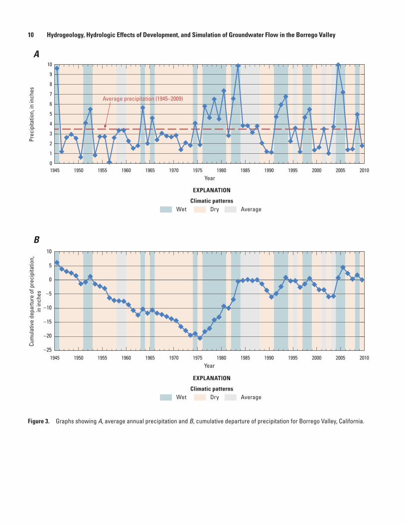
10 Hydrogeology, Hydrologic Effects of Development, and Simulation of Groundwater Flow in the Borrego Valley
Figure 3. Graphs showing A, average annual precipitation and B, cumulative departure of precipitation for Borrego Valley, California.
–25
–20
–15
–10
–5
0
5
10
Cum
ulat
ive
depa
rture
of p
reci
pita
tion,
in in
ches
0
1
2
3
4
5
6
7
8
9
10
1945 1950 1955 1960 1965 1970 1975 1980 1985 1990 1995 2000 2005 2010
Prec
ipita
tion,
in in
ches
Year
1945 1950 1955 1960 1965 1970 1975 1980 1985 1990 1995 2000 2005 2010Year
Average precipitation (1945–2009)
A
B
sac13-0509_Figure 03 Ave precip & departure
Climatic patternsWet Dry Average
EXPLANATION
Climatic patternsWet Dry Average
EXPLANATION
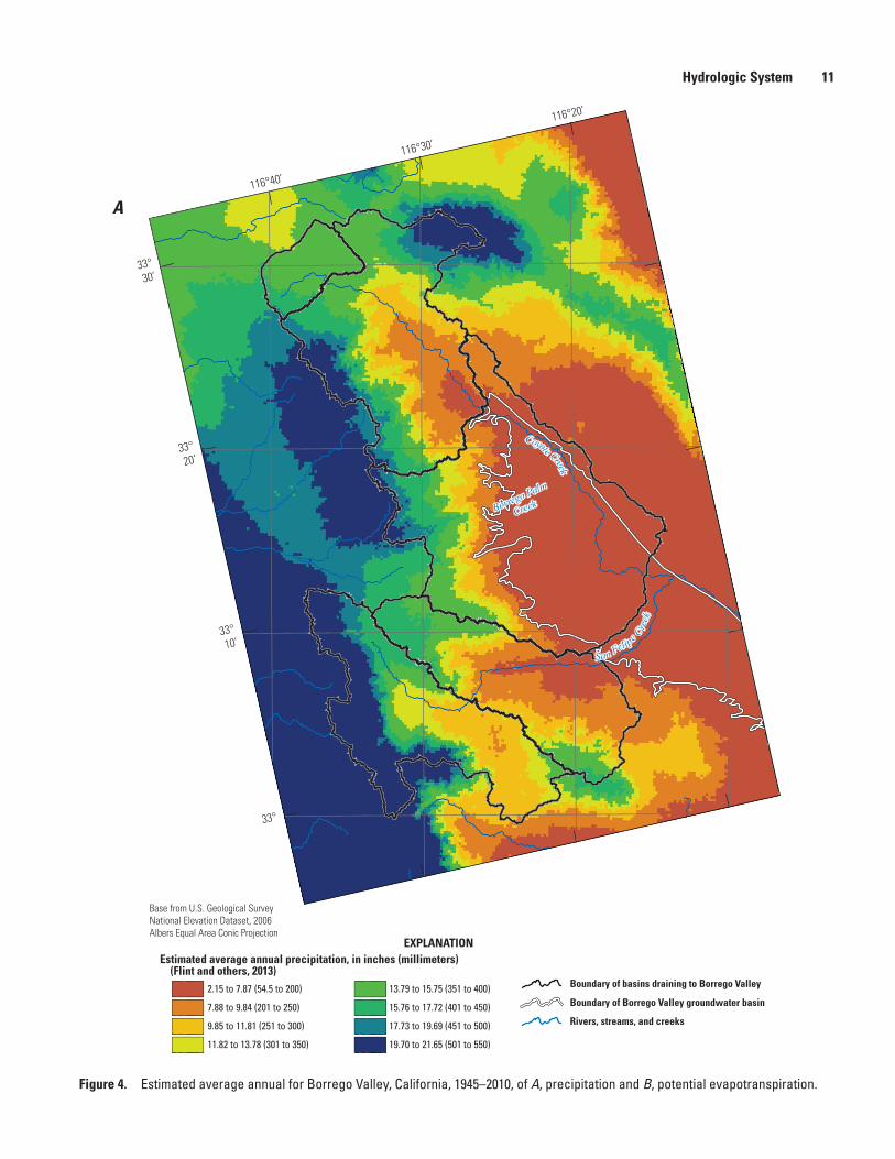
Hydrologic System 11
sac13-0509_Figure 04a_PPT updated
116°20’
116°30’
116°40’
33°30’
33°20’
33°10’
33°
EXPLANATIONEstimated average annual precipitation, in inches (millimeters) (Flint and others, 2013)
2.15 to 7.87 (54.5 to 200) 13.79 to 15.75 (351 to 400)
7.88 to 9.84 (201 to 250) 15.76 to 17.72 (401 to 450)
9.85 to 11.81 (251 to 300) 17.73 to 19.69 (451 to 500)
11.82 to 13.78 (301 to 350) 19.70 to 21.65 (501 to 550)
Boundary of basins draining to Borrego Valley
Rivers, streams, and creeks
Boundary of Borrego Valley groundwater basin
Borrego Palm
Creek
Coyote Creek
San Felipe C
reek
Base from U.S. Geological Survey National Elevation Dataset, 2006Albers Equal Area Conic Projection
A
Figure 4. Estimated average annual for Borrego Valley, California, 1945–2010, of A, precipitation and B, potential evapotranspiration.
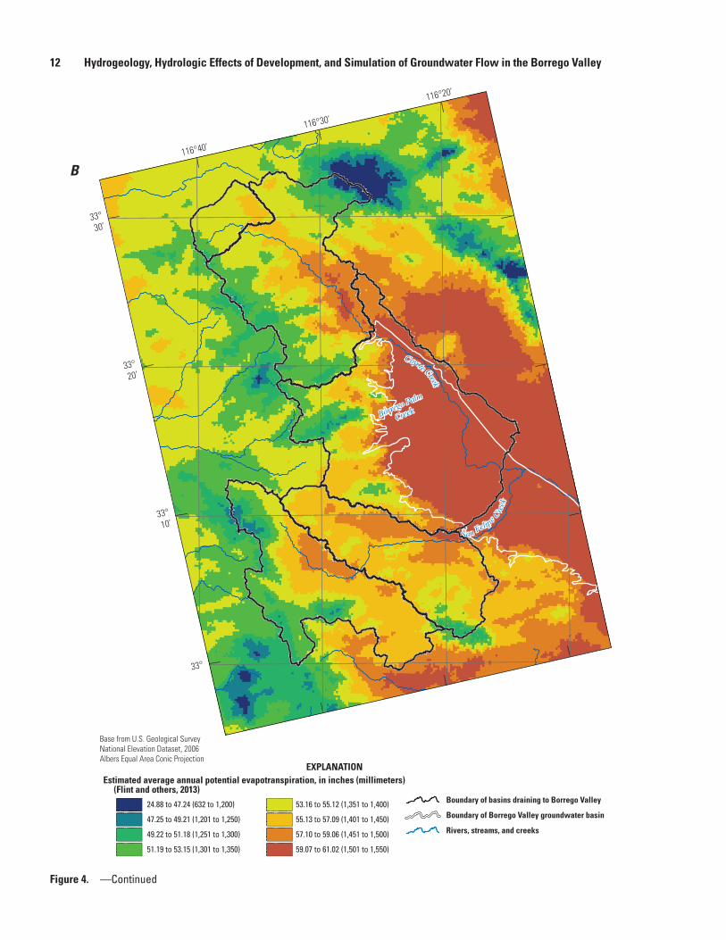
12 Hydrogeology, Hydrologic Effects of Development, and Simulation of Groundwater Flow in the Borrego Valley
sac13-0509_Figure 04b_PET updated
116°20’
116°30’
116°40’
33°30’
33°20’
33°10’
33°
Borrego Palm
Creek
Coyote Creek
San Felip
e C
reek
EXPLANATION
Boundary of basins draining to Borrego Valley
Rivers, streams, and creeks
Boundary of Borrego Valley groundwater basin24.88 to 47.24 (632 to 1,200)
47.25 to 49.21 (1,201 to 1,250)
49.22 to 51.18 (1,251 to 1,300)
51.19 to 53.15 (1,301 to 1,350)
53.16 to 55.12 (1,351 to 1,400)
55.13 to 57.09 (1,401 to 1,450)
57.10 to 59.06 (1,451 to 1,500)
59.07 to 61.02 (1,501 to 1,550)
Estimated average annual potential evapotranspiration, in inches (millimeters) (Flint and others, 2013)
Base from U.S. Geological Survey National Elevation Dataset, 2006Albers Equal Area Conic Projection
B
Figure 4. —Continued
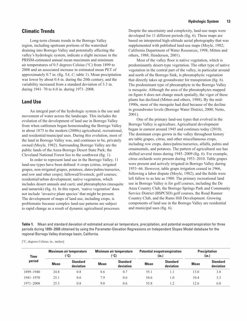
Hydrologic System 13
Climatic Trends
Long-term climate trends in the Borrego Valley region, including upstream portions of the watershed draining into Borrego Valley and potentially affecting the valley’s hydrologic system, indicate a slight increase in the PRISM-estimated annual mean maximum and minimum air temperatures of 0.5 degrees Celsius (°C) from 1899 to 2008 and an associated increase in estimated mean PET of approximately 0.7 in. (fig. 5A, C; table 1). Mean precipitation was lower by about 0.4 in. during the 20th century, and the variability increased from a standard deviation of 3.3 in. during 1941–70 to 6.0 in. during 1971–2008.
Land Use
An integral part of the hydrologic system is the use and movement of water across the landscape. This includes the evolution of the development of land use in Borrego Valley from when cattlemen began homesteading the Borrego Valley in about 1875 to the modern (2000s) agricultural, recreational, and residential/municipal uses. During this evolution, most of the land in Borrego Valley was, and continues to be, privately owned (Moyle, 1982). Surrounding Borrego Valley are the public lands of the Anza-Borrego Desert State Park; the Cleveland National Forest lies to the southwest (fig. 1).
In order to represent land use in the Borrego Valley, 11 land-use types have been defined: 6 crops (citrus, irrigated grapes, non-irrigated grapes, potatoes, dates/palms/nurseries, and row and other crops); fallowed/livestock; golf courses; residential/urban development; native vegetation, which includes desert annuals and cacti; and phreatophytes (mesquite and tamarisk) (fig. 6). In this report, ‘native vegetation’ does not include ‘invasive plant species’ that might be present. The development of maps of land use, including crops, is problematic because complex land-use patterns are subject to rapid change as a result of dynamic agricultural processes.
Despite the uncertainty and complexity, land-use maps were developed for 11 different periods (fig. 6). These maps are based on interpreted high-altitude aerial photography that was supplemented with published land-use maps (Moyle, 1982; California Department of Water Resources, 1998; Mitten and others, 1988; Henderson, 2001).
Most of the valley floor is native vegetation, which is predominantly desert-type vegetation. The other type of native vegetation in the central part of the valley, in particular around and north of the Borrego Sink, is phreatophytic vegetation that directly takes up groundwater for transpiration (fig. 6). The predominant type of phreatophyte in the Borrego Valley is mesquite. Although the area of the phreatophytes mapped on figure 6 does not change much spatially, the vigor of these plants has declined (Mitten and others, 1988). By the mid-1990s, most of the mesquite had died because of the decline in groundwater levels (Borrego Water District, 2000; Netto, 2001).
One of the primary land-use types that evolved in the Borrego Valley is agriculture. Agricultural development began in earnest around 1945 and continues today (2010). The dominant crops grown in the valley throughout history are table grapes, citrus, and other miscellaneous crops, including row crops, dates/palms/nurseries, alfalfa, palms and ornamentals, and potatoes. The pattern of agricultural use has shifted several times during 1945–2009 (fig. 6). For example, citrus orchards were present during 1953–2010. Table grapes were present and actively irrigated in Borrego Valley during 1953–66. However, table grape irrigation ceased in 1966, following a labor dispute (Moyle, 1982), and the fields were left fallow to as late as 1980. The primary recreational land use in Borrego Valley is for golf courses, including the De Anza Country Club, the Borrego Springs Park and Community Service District (BSPCSD) golf courses, the Road Runner Country Club, and the Rams Hill Development. Growing components of land use in the Borrego Valley are residential and municipal uses (fig. 6).
Table 1. Mean and standard deviation of estimated annual air temperature, precipitation, and potential evapotranspiration for three periods during 1899–2008 obtained by using the Parameter-Elevation Regressions on Independent Slopes Model database for the regional Borrego Valley drainage basin, California.
[°C, degrees Celsius; in., inches]
Time period
Maximum air temperature (°C)
Minimum air temperature (°C)
Potential evapotranspiration (in.)
Precipitation (in.)
MeanStandard deviation
MeanStandard deviation
MeanStandard deviation
MeanStandard deviation
1899–1940 24.8 0.8 8.6 0.7 55.1 1.1 13.0 3.8 1941–1970 25.1 0.6 7.9 0.6 54.6 1.0 10.4 3.3 1971–2008 25.3 0.8 9.0 0.6 55.8 1.2 12.6 6.0
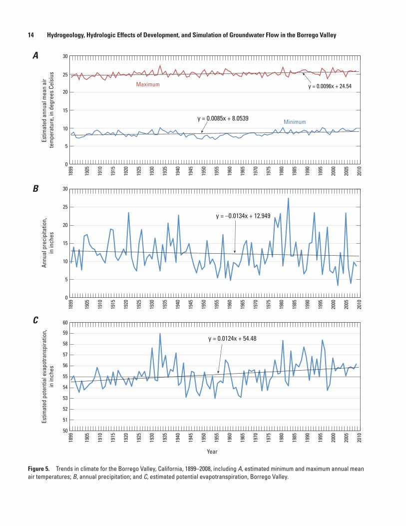
14 Hydrogeology, Hydrologic Effects of Development, and Simulation of Groundwater Flow in the Borrego Valley
Figure 5. Trends in climate for the Borrego Valley, California, 1899–2008, including A, estimated minimum and maximum annual mean air temperatures; B, annual precipitation; and C, estimated potential evapotranspiration, Borrego Valley.
sac13-0509_Figure 05abc climate trends
0
5
10
15
20
25
30
Estim
ated
ann
ual m
ean
air
tem
pera
ture
, in
degr
ees
Cels
ius
Annu
al p
reci
pita
tion,
in in
ches
Es
timat
ed p
oten
tial e
vapo
trans
pira
tion,
in in
ches
Year
A
B
C
1899
1905
1910
1915
1920
1925
1930
1935
1940
1945
1950
1955
1960
1965
1970
1975
1980
1985
1990
1995
2000
2005
2010
0
5
10
15
20
25
30
50
51
52
53
54
55
56
57
59
58
60
1899
1905
1910
1915
1920
1925
1930
1935
1940
1945
1950
1955
1960
1965
1970
1975
1980
1985
1990
1995
2000
2005
2010
1899
1905
1910
1915
1920
1925
1930
1935
1940
1945
1950
1955
1960
1965
1970
1975
1980
1985
1990
1995
2000
2005
2010
y = –0.0134x + 12.949
y = 0.0124x + 54.48
y = 0.0096x + 24.54
y = 0.0085x + 8.0539
Maximum
Minimum
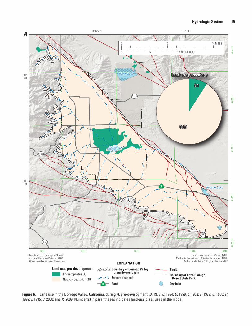
Hydrologic System 15
Figure 6. Land use in the Borrego Valley, California, during A, pre-development; B, 1953; C, 1954; D, 1959; E, 1968; F, 1979; G, 1980; H, 1992; I, 1995; J, 2000; and K, 2009. Number(s) in parentheses indicates land-use class used in the model.
Clark Lake
BorregoSink
Benson Lake
T9S
T10S
T11S
T12S
T13S
R5E R6E R7E R8E R9E
S-22
S-22
S-2
78
116°10’116°20’
33°20’
33°10’
0
0 5 10
5 10 MILES
KILOMETERS
sac13-0509_Figure 06a LU-Predevelopment
A
Stream channel
Boundary of Borrego Valley groundwater basin
Boundary of Anza-Borrego Desert State Park
Land use, pre-developmentPhreatophytes (4)
Native vegetation (15)
Fault
EXPLANATION
Road78
Base from U.S. Geological Survey National Elevation Dataset, 2006Albers Equal Area Conic Projection
Landuse is based on Moyle, 1982; California Department of Water Resources, 1998;
Mitten and others, 1988; Henderson, 2001
Dry lake
Land-use percentage
90.9
9.1
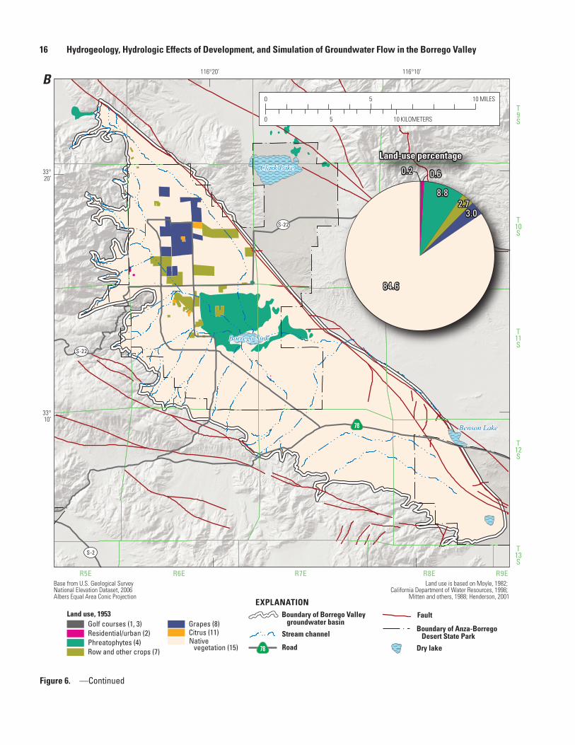
16 Hydrogeology, Hydrologic Effects of Development, and Simulation of Groundwater Flow in the Borrego Valley
Clark Lake
Borrego Sink
Benson Lake
T9S
T10S
T11S
T12S
T13S
R5E R6E R7E R8E R9E
S-22
S-22
S-2
78
116°10’116°20’
33°20’
33°10’
sac13-0509_Figure 06b_LU-1953
B
EXPLANATIONLand use, 1953
Phreatophytes (4) Citrus (11)
Row and other crops (7)
Grapes (8) Residential/urban (2) Golf courses (1, 3)
Native vegetation (15)
Stream channel
FaultBoundary of Borrego Valley groundwater basin
Boundary of Anza-Borrego Desert State Park
0
0 5 10
5 10 MILES
KILOMETERS
Road78
Base from U.S. Geological Survey National Elevation Dataset, 2006Albers Equal Area Conic Projection
Land use is based on Moyle, 1982; California Department of Water Resources, 1998;
Mitten and others, 1988; Henderson, 2001
Dry lake
Land-use percentage
84.6
3.02.7
8.8
0.60.2
Figure 6. —Continued
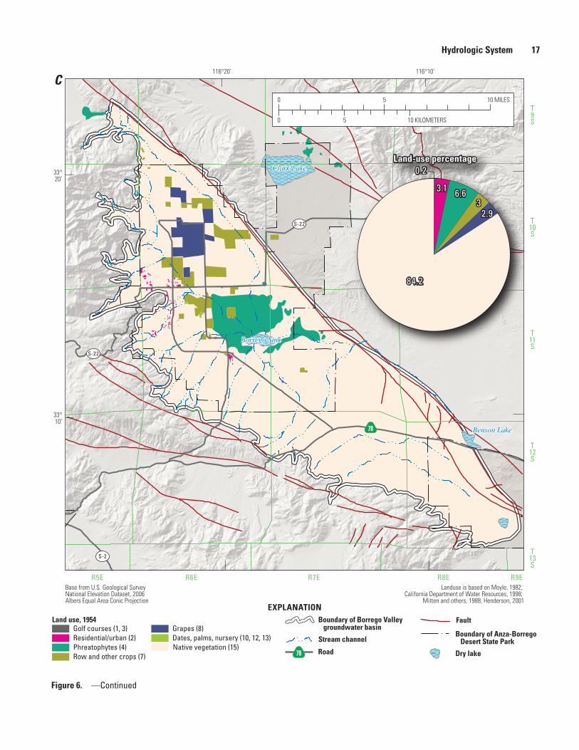
Hydrologic System 17
Clark Lake
Borrego Sink
Benson Lake
T9S
T10S
T11S
T12S
T13S
R5E R6E R7E R8E R9EBase from U.S. Geological Survey National Elevation Dataset, 2006Albers Equal Area Conic Projection
Landuse is based on Moyle, 1982; California Department of Water Resources, 1998;
Mitten and others, 1988; Henderson, 2001
S-22
S-22
S-2
78
116°10’116°20’
33°20’
33°10’
sac13-0509_Figure 06c_LU-1954
C
EXPLANATIONLand use, 1954
Phreatophytes (4) Row and other crops (7)
Residential/urban (2) Golf courses (1, 3)
Dates, palms, nursery (10, 12, 13) Grapes (8)
Native vegetation (15) Stream channel
Boundary of Borrego Valley groundwater basin
0
0 5 10
5 10 MILES
KILOMETERS
Road78
Fault
Boundary of Anza-Borrego Desert State Park
Dry lake
Land-use percentage
84.2
2.9
0.2
3.1 6.63
Figure 6. —Continued
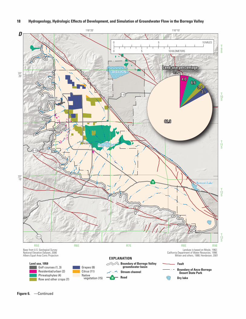
18 Hydrogeology, Hydrologic Effects of Development, and Simulation of Groundwater Flow in the Borrego Valley
Figure 6. —Continued
Clark Lake
Borrego Sink
Benson Lake
T9S
T10S
T11S
T12S
T13S
R5E R6E R7E R8E R9EBase from U.S. Geological Survey National Elevation Dataset, 2006Albers Equal Area Conic Projection
Landuse is based on Moyle, 1982; California Department of Water Resources, 1998;
Mitten and others, 1988; Henderson, 2001
S-22
S-22
S-2
78
116°10’116°20’
33°20’
33°10’
sac13-0509_Figure 06d_LU-1959
D
EXPLANATION
Citrus (11) Grapes (8)
Native vegetation (15)
Land use, 1959
Phreatophytes (4) Row and other crops (7)
Residential/urban (2) Golf courses (1, 3)
Stream channel
Boundary of Borrego Valley groundwater basin
0
0 5 10
5 10 MILES
KILOMETERS
Road78
Fault
Boundary of Anza-Borrego Desert State Park
Dry lake
Land-use percentage
82.9
3.13.0
6.64.0
0.4
De Anza Country Club
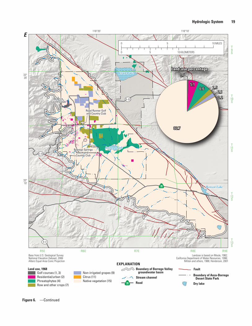
Hydrologic System 19
Figure 6. —Continued
Clark Lake
Borrego Sink
Benson Lake
T9S
T10S
T11S
T12S
T13S
R5E R6E R7E R8E R9EBase from U.S. Geological Survey National Elevation Dataset, 2006Albers Equal Area Conic Projection
Landuse is based on Moyle, 1982; California Department of Water Resources, 1998;
Mitten and others, 1988; Henderson, 2001
S-22
S-22
S-2
78
116°10’116°20’
33°20’
33°10’
sac13-0509_Figure -06e_LU-1968
E
EXPLANATION
0
0 5 10
5 10 MILES
KILOMETERS
Land use, 1968
Phreatophytes (4) Row and other crops (7)
Residential/urban (2) Golf courses (1, 3)
Citrus (11) Non-irrigated grapes (9)
Native vegetation (15) Stream channel
Boundary of Borrego Valley groundwater basin
Road78
Fault
Boundary of Anza-Borrego Desert State Park
Dry lake
Land-use percentage
82.7
2.10.2
2.56.65.1
0.7
De Anza Country Club
Borrego Springs Resort and Country Club
Road Runner Golf and Country Club
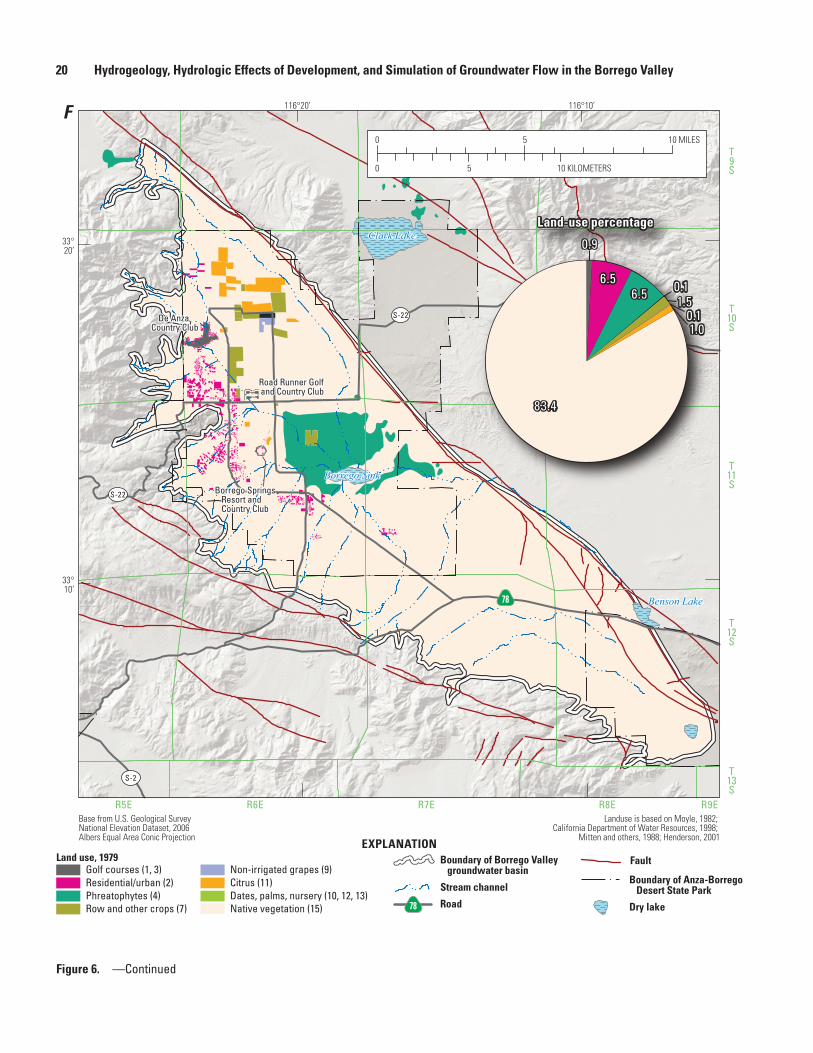
20 Hydrogeology, Hydrologic Effects of Development, and Simulation of Groundwater Flow in the Borrego Valley
Figure 6. —Continued
Clark Lake
Borrego Sink
Benson Lake
T9S
T10S
T11S
T12S
T13S
R5E R6E R7E R8E R9EBase from U.S. Geological Survey National Elevation Dataset, 2006Albers Equal Area Conic Projection
Landuse is based on Moyle, 1982; California Department of Water Resources, 1998;
Mitten and others, 1988; Henderson, 2001
S-22
S-22
S-2
78
116°10’116°20’
33°20’
33°10’
sac13-0509_Figure 06f-LU-1979
F
EXPLANATIONLand use, 1979
Phreatophytes (4) Row and other crops (7)
Residential/urban (2) Golf courses (1, 3)
Citrus (11) Dates, palms, nursery (10, 12, 13)
Non-irrigated grapes (9)
Native vegetation (15)
Stream channel
Boundary of Borrego Valley groundwater basin
Road78
0
0 5 10
5 10 MILES
KILOMETERS
Fault
Boundary of Anza-Borrego Desert State Park
Dry lake
Land-use percentage
83.4
0.9
6.56.5 1.5
1.0
0.1
0.1De Anza Country Club
Borrego Springs Resort and Country Club
Road Runner Golf and Country Club
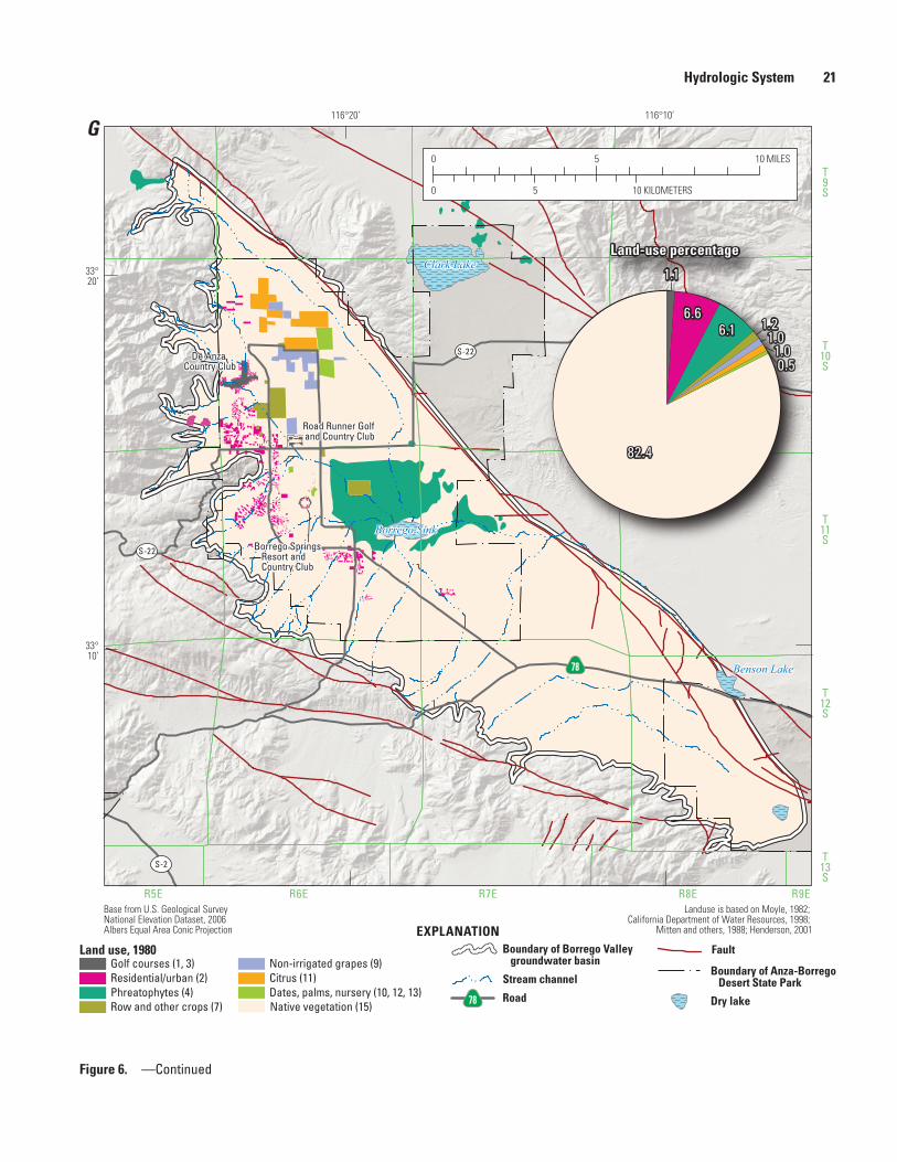
Hydrologic System 21
Figure 6. —Continued
Clark Lake
Borrego Sink
Benson Lake
T9S
T10S
T11S
T12S
T13S
R5E R6E R7E R8E R9EBase from U.S. Geological Survey National Elevation Dataset, 2006Albers Equal Area Conic Projection
Landuse is based on Moyle, 1982; California Department of Water Resources, 1998;
Mitten and others, 1988; Henderson, 2001
S-22
S-22
S-2
78
116°10’116°20’
33°20’
33°10’
sac13-0509_Figure 06g_LU-1980
G
EXPLANATIONLand use, 1980
Phreatophytes (4) Row and other crops (7)
Residential/urban (2) Golf courses (1, 3)
Citrus (11) Dates, palms, nursery (10, 12, 13)
Non-irrigated grapes (9)
Native vegetation (15)
Stream channel
Boundary of Borrego Valley groundwater basin
0
0 5 10
5 10 MILES
KILOMETERS
Road78
Fault
Boundary of Anza-Borrego Desert State Park
Dry lake
Land-use percentage
82.4
1.1
6.66.1 1.2
1.01.00.5
De Anza Country Club
Road Runner Golf and Country Club
Borrego Springs Resort and Country Club
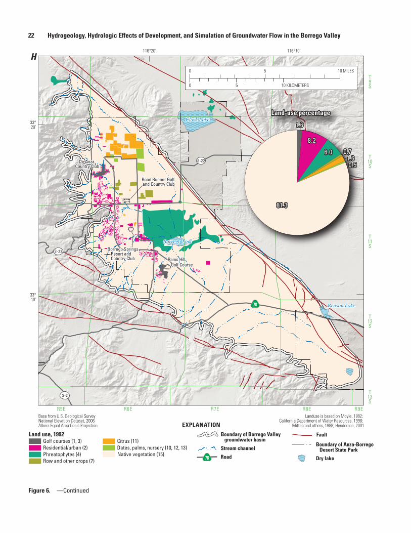
22 Hydrogeology, Hydrologic Effects of Development, and Simulation of Groundwater Flow in the Borrego Valley
Clark Lake
Borrego Sink
Benson Lake
T9S
T10S
T11S
T12S
T13S
S-22
S-22
S-2
78
116°10’116°20’
33°20’
33°10’
sac13-0509_Figure 06h_LU-1992
H
EXPLANATION
Land use, 1992Citrus (11)
Phreatophytes (4) Dates, palms, nursery (10, 12, 13)
Row and other crops (7)
Residential/urban (2) Golf courses (1, 3)
Native vegetation (15) Stream channel
Boundary of Borrego Valley groundwater basin
0
0 5 10
5 10 MILES
KILOMETERS
Road78
R5E R6E R7E R8E R9EBase from U.S. Geological Survey National Elevation Dataset, 2006Albers Equal Area Conic Projection
Landuse is based on Moyle, 1982; California Department of Water Resources, 1998;
Mitten and others, 1988; Henderson, 2001
Fault
Boundary of Anza-Borrego Desert State Park
Dry lake
Land-use percentage
81.3
1.6
8.2
6.0 0.71.60.5De Anza
Country Club
Road Runner Golf and Country Club
Rams Hill Golf Course
Borrego Springs Resort and Country Club
Figure 6. —Continued
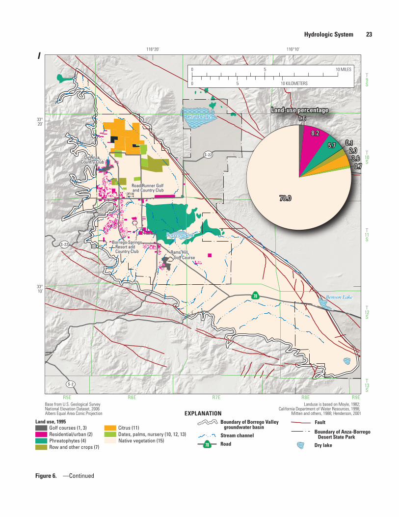
Hydrologic System 23
Clark Lake
Borrego Sink
Benson Lake
T9S
T10S
T11S
T12S
T13S
S-22
S-22
S-2
78
116°10’116°20’
33°20’
33°10’
sac13-0509_Figure 06i_LU-1995
I
EXPLANATIONLand use, 1995
Phreatophytes (4) Row and other crops (7)
Residential/urban (2) Golf courses (1, 3) Citrus (11)
Dates, palms, nursery (10, 12, 13) Native vegetation (15)
Stream channel
Boundary of Borrego Valley groundwater basin
0
0 5 10
5 10 MILES
KILOMETERS
Road78
R5E R6E R7E R8E R9EBase from U.S. Geological Survey National Elevation Dataset, 2006Albers Equal Area Conic Projection
Landuse is based on Moyle, 1982; California Department of Water Resources, 1998;
Mitten and others, 1988; Henderson, 2001
Fault
Boundary of Anza-Borrego Desert State Park
Dry lake
Land-use percentage
78.0
1.6
8.2
5.7 0.12.0
0.73.6De Anza
Country Club
Road Runner Golf and Country Club
Rams Hill Golf Course
Borrego Springs Resort and Country Club
Figure 6. —Continued
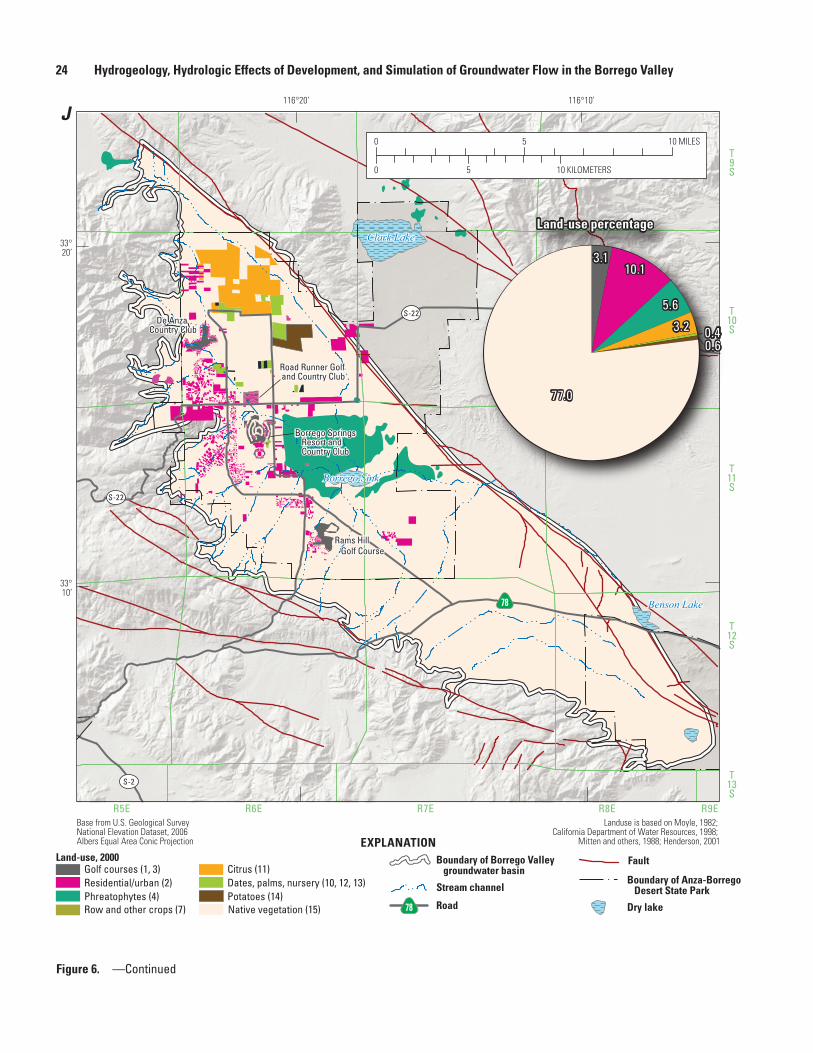
24 Hydrogeology, Hydrologic Effects of Development, and Simulation of Groundwater Flow in the Borrego Valley
Figure 6. —Continued
Clark Lake
Borrego Sink
Benson Lake
T9S
T10S
T11S
T12S
T13S
R5E R6E R7E R8E R9EBase from U.S. Geological Survey National Elevation Dataset, 2006Albers Equal Area Conic Projection
Landuse is based on Moyle, 1982; California Department of Water Resources, 1998;
Mitten and others, 1988; Henderson, 2001
S-22
S-22
S-2
78
116°10’116°20’
33°20’
33°10’
sac13-0509_Figure 06j_LU-2000
J
EXPLANATION
0
0 5 10
5 10 MILES
KILOMETERS
Road78
Land-use percentage
Land-use, 2000
Phreatophytes (4) Row and other crops (7)
Residential/urban (2) Golf courses (1, 3) Citrus (11)
Dates, palms, nursery (10, 12, 13) Potatoes (14) Native vegetation (15)
Stream channel
Boundary of Borrego Valley groundwater basin
77.0
3.110.1
5.6
3.2 0.40.6
Fault
Boundary of Anza-Borrego Desert State Park
Dry lake
De Anza Country Club
Borrego Springs Resort and Country Club
Road Runner Golf and Country Club
Rams Hill Golf Course
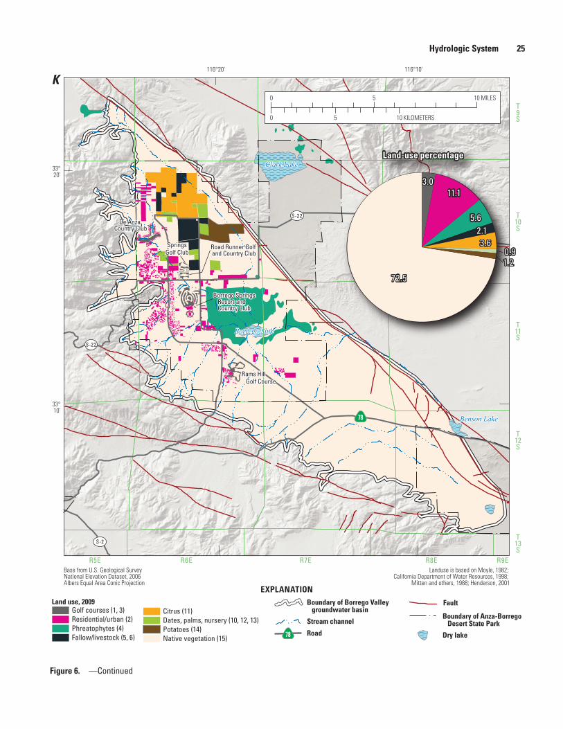
Hydrologic System 25
Figure 6. —Continued
Clark Lake
Borrego Sink
Benson Lake
T9S
T10S
T11S
T12S
T13S
R5E R6E R7E R8E R9EBase from U.S. Geological Survey National Elevation Dataset, 2006Albers Equal Area Conic Projection
Landuse is based on Moyle, 1982; California Department of Water Resources, 1998;
Mitten and others, 1988; Henderson, 2001
S-22
S-22
S-2
78
116°10’116°20’
33°20’
33°10’
sac13-0509_Figure 06k_LU-2009
K
Rams Hill Golf Course
De Anza Country Club
Borrego Springs Resort and Country Club
Road Runner Golf and Country Club
SpringsGolf Club
EXPLANATIONLand use, 2009
Citrus (11)
Phreatophytes (4) Dates, palms, nursery (10, 12, 13) Potatoes (14)
Fallow/livestock (5, 6)
Residential/urban (2) Golf courses (1, 3)
Native vegetation (15)
Stream channel
Boundary of Borrego Valley groundwater basin
0
0 5 10
5 10 MILES
KILOMETERS
Road78
Fault
Boundary of Anza-Borrego Desert State Park
Dry lake
Land-use percentage
72.5
11.1
5.62.13.6
0.91.2
3.0
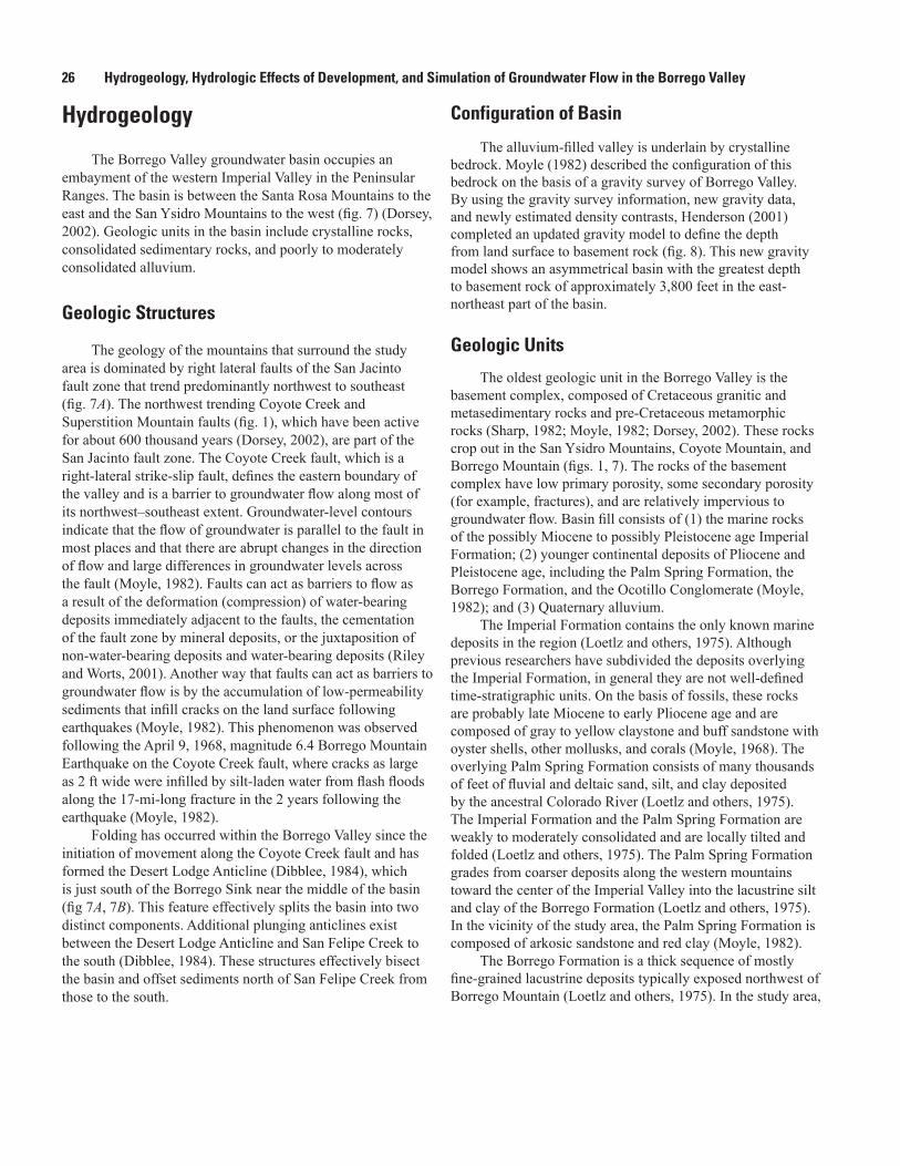
26 Hydrogeology, Hydrologic Effects of Development, and Simulation of Groundwater Flow in the Borrego Valley
Hydrogeology
The Borrego Valley groundwater basin occupies an embayment of the western Imperial Valley in the Peninsular Ranges. The basin is between the Santa Rosa Mountains to the east and the San Ysidro Mountains to the west (fig. 7) (Dorsey, 2002). Geologic units in the basin include crystalline rocks, consolidated sedimentary rocks, and poorly to moderately consolidated alluvium.
Geologic Structures
The geology of the mountains that surround the study area is dominated by right lateral faults of the San Jacinto fault zone that trend predominantly northwest to southeast (fig. 7A). The northwest trending Coyote Creek and Superstition Mountain faults (fig. 1), which have been active for about 600 thousand years (Dorsey, 2002), are part of the San Jacinto fault zone. The Coyote Creek fault, which is a right-lateral strike-slip fault, defines the eastern boundary of the valley and is a barrier to groundwater flow along most of its northwest–southeast extent. Groundwater-level contours indicate that the flow of groundwater is parallel to the fault in most places and that there are abrupt changes in the direction of flow and large differences in groundwater levels across the fault (Moyle, 1982). Faults can act as barriers to flow as a result of the deformation (compression) of water-bearing deposits immediately adjacent to the faults, the cementation of the fault zone by mineral deposits, or the juxtaposition of non-water-bearing deposits and water-bearing deposits (Riley and Worts, 2001). Another way that faults can act as barriers to groundwater flow is by the accumulation of low-permeability sediments that infill cracks on the land surface following earthquakes (Moyle, 1982). This phenomenon was observed following the April 9, 1968, magnitude 6.4 Borrego Mountain Earthquake on the Coyote Creek fault, where cracks as large as 2 ft wide were infilled by silt-laden water from flash floods along the 17-mi-long fracture in the 2 years following the earthquake (Moyle, 1982).
Folding has occurred within the Borrego Valley since the initiation of movement along the Coyote Creek fault and has formed the Desert Lodge Anticline (Dibblee, 1984), which is just south of the Borrego Sink near the middle of the basin (fig 7A, 7B). This feature effectively splits the basin into two distinct components. Additional plunging anticlines exist between the Desert Lodge Anticline and San Felipe Creek to the south (Dibblee, 1984). These structures effectively bisect the basin and offset sediments north of San Felipe Creek from those to the south.
Configuration of Basin
The alluvium-filled valley is underlain by crystalline bedrock. Moyle (1982) described the configuration of this bedrock on the basis of a gravity survey of Borrego Valley. By using the gravity survey information, new gravity data, and newly estimated density contrasts, Henderson (2001) completed an updated gravity model to define the depth from land surface to basement rock (fig. 8). This new gravity model shows an asymmetrical basin with the greatest depth to basement rock of approximately 3,800 feet in the east-northeast part of the basin.
Geologic Units
The oldest geologic unit in the Borrego Valley is the basement complex, composed of Cretaceous granitic and metasedimentary rocks and pre-Cretaceous metamorphic rocks (Sharp, 1982; Moyle, 1982; Dorsey, 2002). These rocks crop out in the San Ysidro Mountains, Coyote Mountain, and Borrego Mountain (figs. 1, 7). The rocks of the basement complex have low primary porosity, some secondary porosity (for example, fractures), and are relatively impervious to groundwater flow. Basin fill consists of (1) the marine rocks of the possibly Miocene to possibly Pleistocene age Imperial Formation; (2) younger continental deposits of Pliocene and Pleistocene age, including the Palm Spring Formation, the Borrego Formation, and the Ocotillo Conglomerate (Moyle, 1982); and (3) Quaternary alluvium.
The Imperial Formation contains the only known marine deposits in the region (Loetlz and others, 1975). Although previous researchers have subdivided the deposits overlying the Imperial Formation, in general they are not well-defined time-stratigraphic units. On the basis of fossils, these rocks are probably late Miocene to early Pliocene age and are composed of gray to yellow claystone and buff sandstone with oyster shells, other mollusks, and corals (Moyle, 1968). The overlying Palm Spring Formation consists of many thousands of feet of fluvial and deltaic sand, silt, and clay deposited by the ancestral Colorado River (Loetlz and others, 1975). The Imperial Formation and the Palm Spring Formation are weakly to moderately consolidated and are locally tilted and folded (Loetlz and others, 1975). The Palm Spring Formation grades from coarser deposits along the western mountains toward the center of the Imperial Valley into the lacustrine silt and clay of the Borrego Formation (Loetlz and others, 1975). In the vicinity of the study area, the Palm Spring Formation is composed of arkosic sandstone and red clay (Moyle, 1982).
The Borrego Formation is a thick sequence of mostly fine-grained lacustrine deposits typically exposed northwest of Borrego Mountain (Loetlz and others, 1975). In the study area,
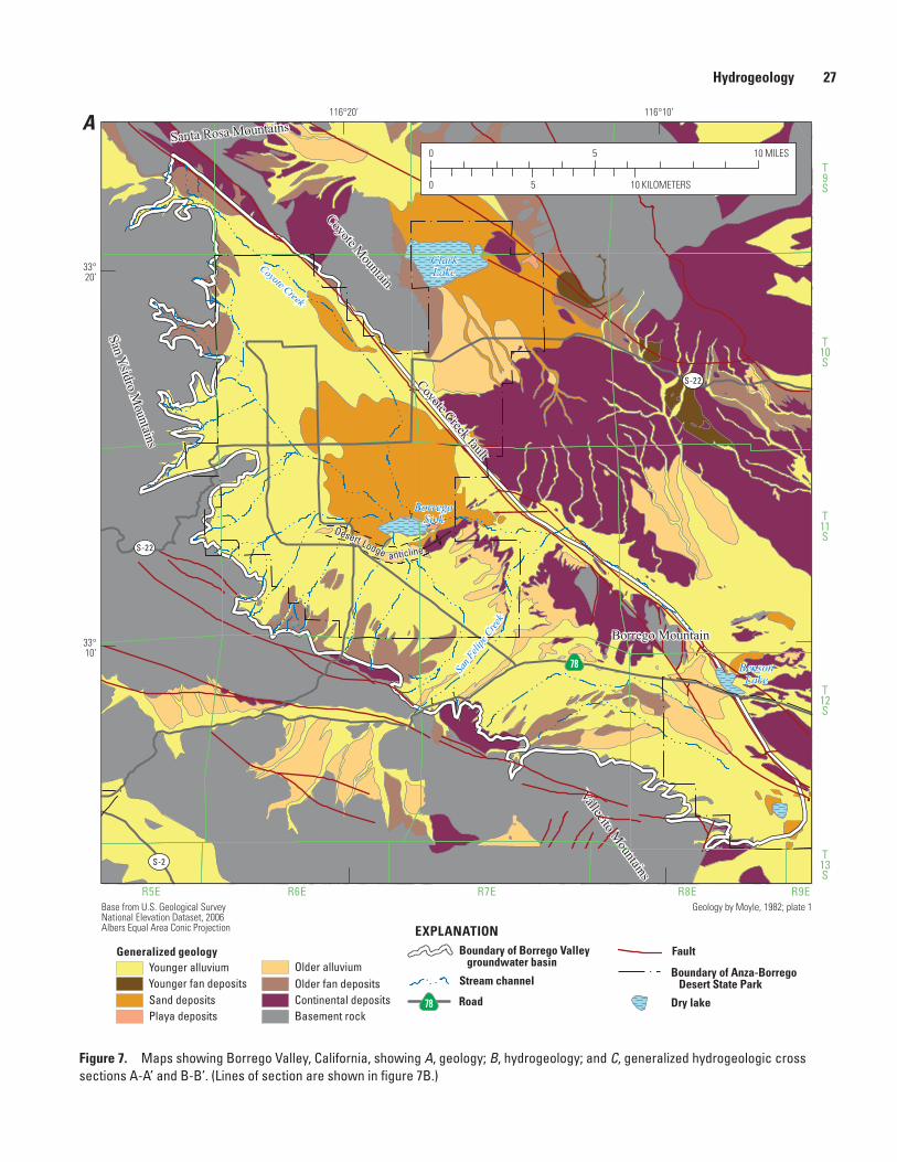
Hydrogeology 27
Vallecito Mountains
ClarkLake
BorregoSink
BensonLake
T9S
T10S
T11S
T12S
T13S
R5E R6E R7E R8E R9EBase from U.S. Geological Survey National Elevation Dataset, 2006Albers Equal Area Conic Projection
Geology by Moyle, 1982; plate 1
S-22
S-22
S-2
78
116°10’116°20’
33°20’
33°10’
0
0 5 10
5 10 MILES
KILOMETERS
sac13-0509_Figure 07a_Geology
Coyote Creek fault
Coyote Mountain
Borrego Mountain
San Ysidro M
ountains
Santa Rosa MountainsA
EXPLANATION
Desert Lodge anticline
Basement rockPlaya depositsContinental deposits Sand deposits
Older alluviumYounger alluviumOlder fan depositsYounger fan deposits
Generalized geology
Stream channel
Boundary of Borrego Valley groundwater basin
Road78
Coyote Creek
San F
elipe
Cree
k
Fault
Boundary of Anza-Borrego Desert State Park
Dry lake
Figure 7. Maps showing Borrego Valley, California, showing A, geology; B, hydrogeology; and C, generalized hydrogeologic cross sections A-A’ and B-B’. (Lines of section are shown in figure 7B.)
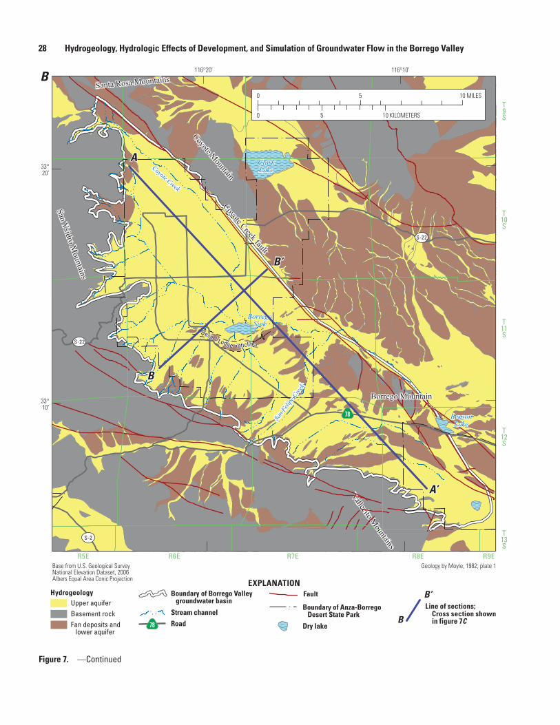
28 Hydrogeology, Hydrologic Effects of Development, and Simulation of Groundwater Flow in the Borrego Valley
Vallecito Mountains
ClarkLake
BorregoSink
BensonLake
T9S
T10S
T11S
T12S
T13S
S-22
S-22
S-2
78
A
A’
B
B’
116°10’116°20’
33°20’
33°10’
0
0 5 10
5 10 MILES
KILOMETERS
sac13-0509_Figure 07b_hydro geo
Coyote Creek fault
Coyote Mountain
Borrego Mountain
San Ysidro M
ountains
Santa Rosa MountainsB
EXPLANATION
Desert Lodge anticline
Basement rockFan deposits and lower aquifer
Upper aquiferHydrogeology
Stream channel
Boundary of Borrego Valley groundwater basin
Line of sections;
B
B’
Cross section shown in figure 7CRoad78
R5E R6E R7E R8E R9EBase from U.S. Geological Survey National Elevation Dataset, 2006Albers Equal Area Conic Projection
Geology by Moyle, 1982; plate 1
Coyote Creek
San F
elipe
Cree
k
Fault
Boundary of Anza-Borrego Desert State Park
Dry lake
Figure 7. —Continued
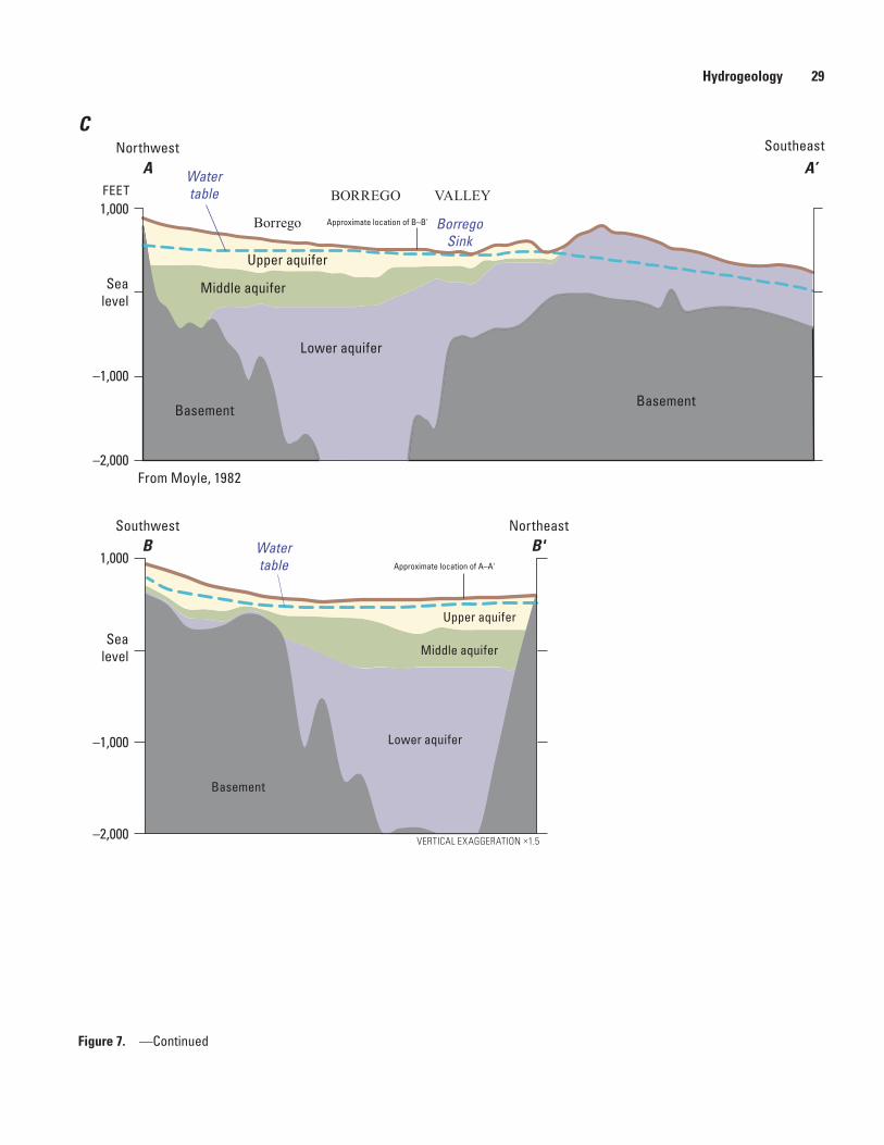
Hydrogeology 29
Figure 7. —Continued
NortheastSouthwest
–2,000
–1,000
Sealevel
1,000B'B
Upper aquifer
Watertable
Middle aquifer
Lower aquifer
Basement
Approximate location of A–A'
Northwest Southeast
–2,000
–1,000
Sealevel
1,000
A A’FEET
VERTICAL EXAGGERATION ×1.5
sac13-0509_Figure 07cd_xsecs AA’ and BB’
C
BORREGO VALLEY
Borrego
Upper aquifer
BorregoSink
Watertable
Middle aquifer
Lower aquifer
BasementBasement
From Moyle, 1982
Approximate location of B–B'
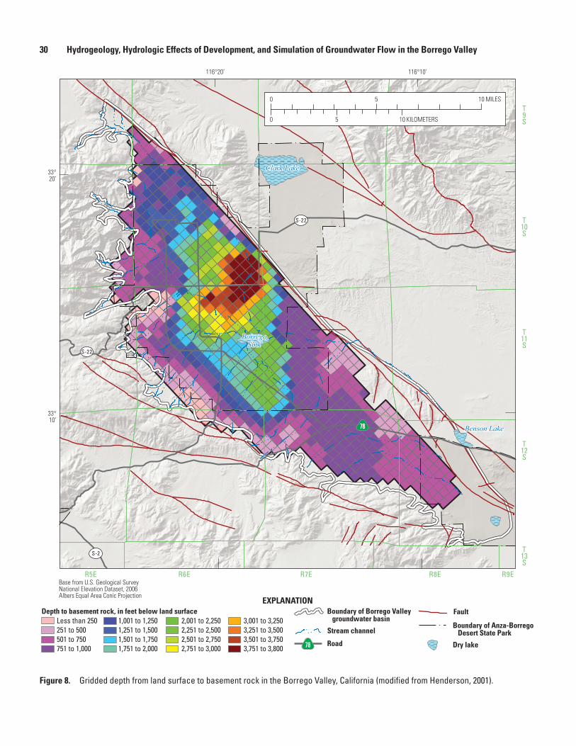
30 Hydrogeology, Hydrologic Effects of Development, and Simulation of Groundwater Flow in the Borrego Valley
Figure 8. Gridded depth from land surface to basement rock in the Borrego Valley, California (modified from Henderson, 2001).
Clark Lake
BorregoSink
Benson Lake
T9S
T10S
T11S
T12S
T13S
R5E R6E R7E R8E R9E
S-22
S-22
S-2
78
116°10’116°20’
33°20’
33°10’
sac13-0509_Figure 08 depth-to-basement
EXPLANATION
0
0 5 10
5 10 MILES
KILOMETERS
Depth to basement rock, in feet below land surfaceLess than 250251 to 500501 to 750751 to 1,000
1,001 to 1,2501,251 to 1,5001,501 to 1,7501,751 to 2,000
2,001 to 2,2502,251 to 2,5002,501 to 2,7502,751 to 3,000
3,001 to 3,2503,251 to 3,5003,501 to 3,7503,751 to 3,800
Stream channel
Boundary of Borrego Valley groundwater basin
Road78
Base from U.S. Geological Survey National Elevation Dataset, 2006Albers Equal Area Conic Projection
Fault
Boundary of Anza-Borrego Desert State Park
Dry lake
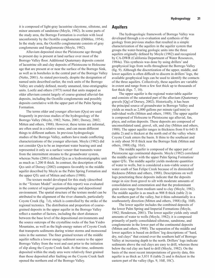
Hydrogeology 31
it is composed of light-gray lacustrine claystone, siltstone, and minor amounts of sandstone (Moyle, 1982). In some parts of the study area, the Borrego Formation is overlain with local unconformity by the Ocotillo conglomerate (Dibblee, 1954). In the study area, the Ocotillo conglomerate consists of gray conglomerate and fanglomerate (Moyle, 1982).
Alluvium deposited since the Pleistocene age through to present day is present at land surface over most of the Borrego Valley floor. Additional Quaternary deposits consist of lacustrine silt and clay deposits of Pleistocene to Holocene age that are present at or near the surface of the Borrego Sink, as well as in boreholes in the central part of the Borrego Valley (Netto, 2001). As stated previously, despite the designation of named units described earlier, the rock units of the Borrego Valley are crudely defined, mostly unnamed, time-stratigraphic units. Loetlz and others (1975) noted that units mapped as older alluvium consist largely of coarse-grained alluvial-fan deposits, including the Ocotillo conglomerate and possibly deposits correlative with the upper part of the Palm Spring Formation.
The terms older and younger alluvium (Qya) are used frequently in previous studies of the hydrogeology of the Borrego Valley (Moyle, 1982; Netto, 2001; Dorsey, 2002; Mitten and others, 1988). However, these terms are informal, are often used in a relative sense, and can mean different things to different authors. In previous hydrogeologic studies of the Borrego Valley, authors have made conflicting characterizations of the younger alluvium. Moyle (1982) did not consider Qya to be an important water bearing unit and represented it only as a surface veneer that transmits water from the intermittent streams to the groundwater system, whereas Netto (2001) defined Qya as a hydrostratigraphic unit as much as 1,200 ft thick. In contrast, the description of the Qcs unit of Dorsey (2002) compares favorably to the middle aquifer described by Moyle as the Palm Spring Formation and the upper QTc unit of Mitten and others (1988).
The texture model developed for this study (described in the “Texture Model” section of this report) was evaluated in the context of regional geomorphology and depositional environment. The spatial structure of the texture model can be attributed to the alignment of the river channels, particularly Coyote Creek (fig. 7A), which is controlled by the strike of the regional tectonics. The distribution and proportion of coarse-grained deposits in the upper aquifer in the Borrego Valley reflect a number of factors, including the short distances between the base level of the depositional environments and the source outcrops of the crystalline rocks of the San Ysidro Mountains, as well as the high-energy nature of Coyote Creek that transports sediments during winter storms and monsoonal rains in the summer. The finer grained texture of the middle aquifer reflects a lower energy sediment source to the upper Borrego Valley from the west and east prior to the initiation of slip along the Coyote Creek fault. At that time, sediments deposited within the study area were relatively finer grained than those deposited after faulting on the Coyote Creek fault opened the northern end of the Borrego Valley.
AquifersThe hydrogeologic framework of Borrego Valley was
developed through a re-evaluation and synthesis of the geology from previous studies that resulted in a simple characterization of the aquifers in the aquifer system that groups the water-bearing geologic units into the three aquifers originally defined by Moyle (1982) and recognized by CA-DWR (California Department of Water Resources, 1984a). This synthesis was done by using drillers’ and geophysical logs from wells throughout the Borrego Valley (fig. 9). Although the discretization of the upper, middle, and lower aquifers is often difficult to discern in drillers’ logs, the available geophysical logs can be used to identify the contacts of the three aquifers. Collectively, these aquifers are variable in extent and range from a few feet thick up to thousands of feet thick (figs. 7, 10).
The upper aquifer is the regional water-table aquifer and consists of the saturated part of the alluvium (Quaternary gravels [Qg] of Dorsey, 2002). Historically, it has been the principal source of groundwater in Borrego Valley and yields as much as 2,000 gallons per minute (gal/min) to individual wells (Mitten and others, 1988). The upper aquifer is composed of Holocene to Pleistocene age alluvial, fan, playa, and eolian deposits. These deposits are composed of unconsolidated sand, gravel, silt, and clay (Mitten and others, 1988). The upper aquifer ranges in thickness from 0 to 643 ft (table 2) and is thickest at the north end of the valley where Coyote Creek enters the basin. It thins to the southeast and is only about 50 ft thick near the Borrego Sink (Mitten and others, 1988) (fig. 10A).
The middle aquifer is composed of the upper part of Pleistocene age continental deposits. Moyle (1982) correlated the middle aquifer with the upper Palm Spring Formation/upper QTc. The middle aquifer yields moderate quantities of water to wells, but is considered a non-viable source of water south of San Felipe Creek because of its diminished thickness (Mitten and others, 1988). Descriptions on well logs penetrating these deposits indicate that the deposits range in size from gravel to silt with moderate amounts of consolidation and cementation and that the predominant grain sizes range from medium sand to clay (Moyle, 1982). The middle aquifer is as much as 908 ft thick (table 2) in the northern part of the valley, but it thins substantially in a southeasterly direction (Mitten and others, 1988) (fig. 10B).
The lower aquifer includes the combined deposits of the lower Palm Spring and Imperial Formations (Moyle, 1982; Henderson, 2001). The lower aquifer yields only small amounts of water to wells (Moyle, 1982); it is composed primarily of partly consolidated siltstone, sandstone, and conglomerate in the lower part of the continental deposits (Mitten and others, 1988). The separation of the middle and lower aquifers is based on drillers’ log descriptions of “hard, dry, red clays” that extend over the southern half of Borrego Valley at increasing depth to the north. Drillers’ logs indicate sediments above the red clays are easy to drill, whereas those below the red clay are hard to drill (Moyle, 1982). On the basis of the most recent interpretations of gravity data, this aquifer is as thick as 3,831 ft (table 2) and is thickest in the eastern part of the valley (figs. 9, 10B, 10C).
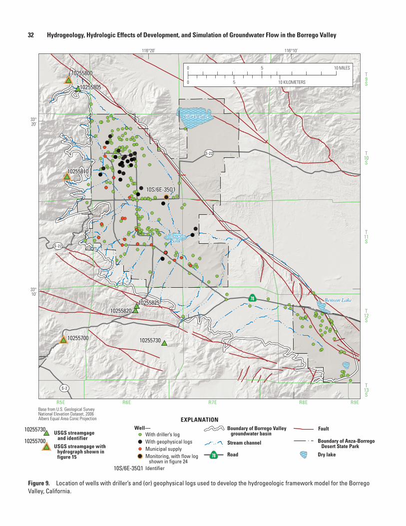
32 Hydrogeology, Hydrologic Effects of Development, and Simulation of Groundwater Flow in the Borrego Valley
Figure 9. Location of wells with driller’s and (or) geophysical logs used to develop the hydrogeologic framework model for the Borrego Valley, California.
Clark Lake
BorregoSink
Benson Lake
T9S
T10S
T11S
T12S
T13S
R5E R6E R7E R8E R9E
S-22
S-22
S-2
7810255825
10255730
10255820
10255810
10S/6E-35Q1
10255805
10255800
10255700
116°10’116°20’
33°20’
33°10’
sac13-0509_Figure 09 Wells & gages
EXPLANATION
0
0 5 10
5 10 MILES
KILOMETERS
With driller’s log
Monitoring, with flow log shown in figure 24
Well—10255730 USGS streamgage and identifier
USGS streamgage with hydrograph shown in figure 15
Municipal supplyWith geophysical logs Stream channel
FaultBoundary of Borrego Valley groundwater basin
Boundary of Anza-Borrego Desert State Park
Road78
10255700
10S/6E-35Q1 Identifier
Base from U.S. Geological Survey National Elevation Dataset, 2006Albers Equal Area Conic Projection
Dry lake
Hydrogeology 33
Figure 10. Extent and approximate thickness of aquifers in Borrego Valley, California, A, upper; B, middle; and C, lower.
Clark Lake
Benson Lake
T9S
T10S
T11S
T12S
T13S
R5E R6E R7E R8E R9EBase from U.S. Geological Survey National Elevation Dataset, 2006Albers Equal Area Conic Projection
S-22
S-22
S-2
78
116°10’116°20’
33°20’
33°10’
sac13-0509_Figure 10a_Thickness_upper
A
EXPLANATION
201 to 300
50 to 100 301 to 400 501 to 600101 to 200 401 to 500 601 to 643
Boundary of layer 1
Approximate thickness of upper aquifer (layer 1), in feet(Thickness of aquifers are not shown where less than 50 feet)
Stream channel
FaultBoundary of Borrego Valley groundwater basin
Boundary of Anza-Borrego Desert State Park
Road78
Dry lake
0
0 5 10
5 10 MILES
KILOMETERS
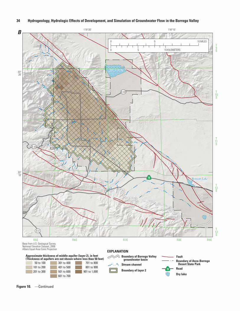
34 Hydrogeology, Hydrologic Effects of Development, and Simulation of Groundwater Flow in the Borrego Valley
Clark Lake
Benson Lake
T9S
T10S
T11S
T12S
T13S
R5E R6E R7E R8E R9EBase from U.S. Geological Survey National Elevation Dataset, 2006Albers Equal Area Conic Projection
S-22
S-22
S-2
78
116°10’116°20’
33°20’
33°10’
sac13-0509_Figure 10b_thickness_middle
B
EXPLANATION
0
0 5 10
5 10 MILES
KILOMETERS
50 to 100101 to 200201 to 300
301 to 400401 to 500501 to 600601 to 700
701 to 800
901 to 1,000801 to 900
Approximate thickness of middle aquifer (layer 2), in feet(Thickness of aquifers are not shown where less than 50 feet)
Boundary of layer 2
Stream channel
Boundary of Borrego Valley groundwater basin Boundary of Anza-Borrego
Desert State Park
Fault
Road78
Dry lake
Figure 10. —Continued
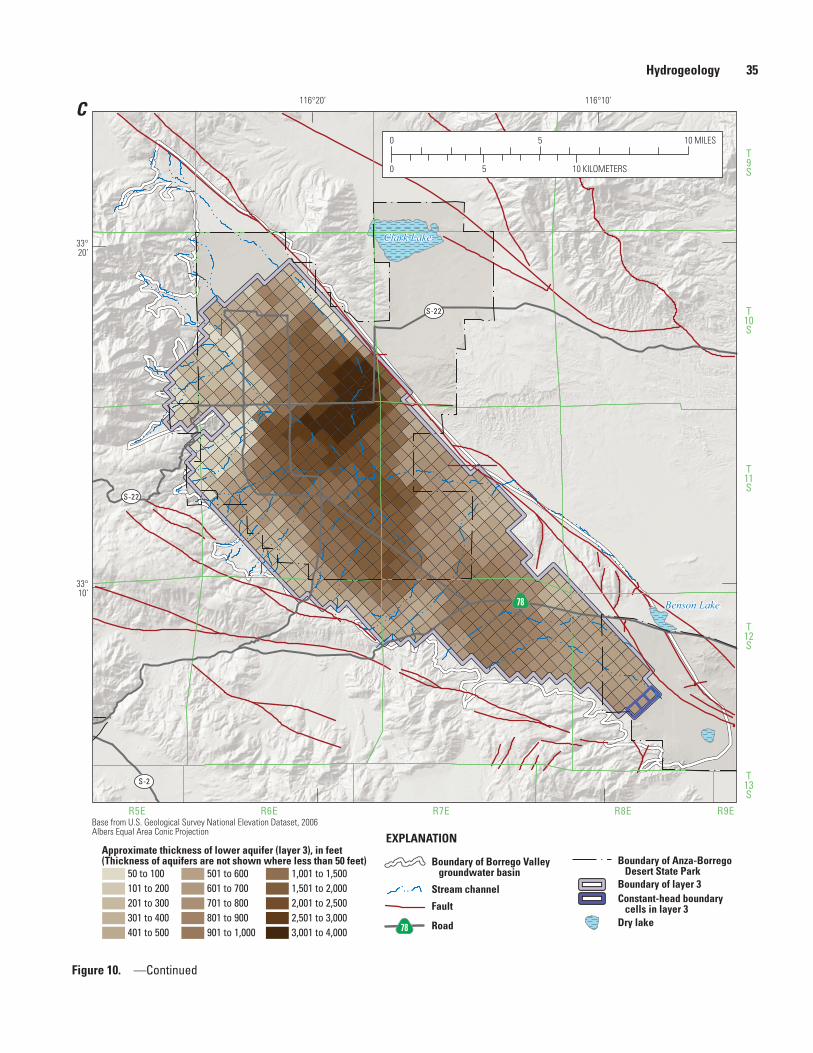
Hydrogeology 35
Clark Lake
Benson Lake
T9S
T10S
T11S
T12S
T13S
R5E R6E R7E R8E R9EBase from U.S. Geological Survey National Elevation Dataset, 2006Albers Equal Area Conic Projection
S-22
S-22
S-2
78
116°10’116°20’
33°20’
33°10’
sac13-0509_Figure 10c_Thickness_lower
C
EXPLANATION
Constant-head boundary cells in layer 3
Approximate thickness of lower aquifer (layer 3), in feet(Thickness of aquifers are not shown where less than 50 feet)
201 to 300 701 to 800 2,001 to 2,500101 to 200 601 to 700 1,501 to 2,00050 to 100 501 to 600 1,001 to 1,500
401 to 500 3,001 to 4,000901 to 1,000301 to 400 2,501 to 3,000801 to 900
Boundary of layer 3Stream channel
Fault
Boundary of Borrego Valley groundwater basin
Boundary of Anza-Borrego Desert State Park
0
0 5 10
5 10 MILES
KILOMETERS
Road78 Dry lake
Figure 10. —Continued
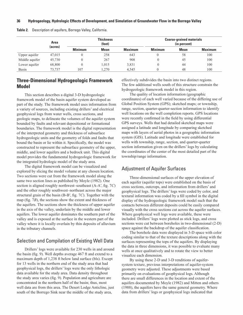
36 Hydrogeology, Hydrologic Effects of Development, and Simulation of Groundwater Flow in the Borrego Valley
Three-Dimensional Hydrogeologic Framework Model
This section describes a digital 3-D hydrogeologic framework model of the basin aquifer system developed as part of the study. The framework model uses information from a variety of sources, including existing drillers’ and electrical geophysical logs from water wells, cross sections, and geologic maps, to delineate the volumes of the aquifer system bounded by faults and relevant depositional or formational boundaries. The framework model is the digital representation of the interpreted geometry and thickness of subsurface hydrogeologic units and the geometry of folds and faults that bound the basin or lie within it. Specifically, the model was constructed to represent the subsurface geometry of the upper, middle, and lower aquifers and a bedrock unit. This digital model provides the fundamental hydrogeologic framework for the integrated hydrologic model of the study area.
The digital framework model can be visualized and explored by slicing the model volume at any chosen location. Two sections were cut from the framework model along the same two section lines as published by Moyle (1982). One section is aligned roughly northwest–southeast (A-A′, fig. 7C) and the other roughly southwest–northeast across the major structural grain of the basin (B-B′, fig. 7C). Together with the map (fig. 7B), the sections show the extent and thickness of the aquifers. The sections show the thickness of upper aquifer in the axis of the valley, underlain by the middle and lower aquifers. The lower aquifer dominates the southern part of the valley and is exposed at the surface in the western part of the valley where it is locally overlain by thin deposits of alluvium in the tributary channels.
Selection and Compilation of Existing Well DataDrillers’ logs were available for 230 wells in and around
the basin (fig. 9). Well depths average 467 ft and extend to a maximum depth of 1,238 ft below land surface (bls). Except for 13 wells in the northern end of the study area that had geophysical logs, the drillers’ logs were the only lithologic data available for the study area. Data density throughout the study area varies (fig. 9). Population and agriculture are concentrated in the northern half of the basin; thus, most well data are from this area. The Desert Lodge Anticline, just south of the Borrego Sink near the middle of the study area,
effectively subdivides the basin into two distinct regions. The few additional wells south of this structure constrain the hydrogeologic framework model in this region.
The quality of location information (geographic coordinates) of each well varied because of the differing use of Global Position System (GPS); sketched maps; or township, range, section, quarter-quarter-section information to identify well locations on the well completion reports. GPS locations were recently confirmed in the field by using differential GPS surveys. Wells that had detailed sketched maps were assigned a latitude and longitude by comparing sketched maps with layers of aerial photos in a geographic information system (GIS). Latitude and longitude were established for wells with township, range, section, and quarter-quarter section information given on the drillers’ logs by calculating the coordinates of the center of the most detailed part of the township/range information.
Adjustment of Aquifer Surfaces
Three-dimensional surfaces of the upper elevation of each aquifer (aquifer tops) were established on the basis of cross sections, outcrops, and information from drillers’ and geophysical logs. The drillers’ logs were coded by color, and textural information was coded by a fill symbol in the digital display of the hydrogeologic framework model such that the contacts between different deposits could be easily compared visually with the cross sections cut across the aquifer surfaces. Where geophysical well logs were available, these were included. Drillers’ logs were plotted as stick logs, and cross sections were cut between boreholes in two-dimensional (2-D) space against the backdrop of the aquifer classification.
The borehole data were displayed in 3-D space with color coding similar to that of the texture descriptions along with the surfaces representing the tops of the aquifers. By displaying the data in three dimensions, it was possible to evaluate many wells at once qualitatively and to rotate the view to better visualize each dimension.
By using these 2-D and 3-D renditions of aquifer-system texture, previous interpretations of aquifer-system geometry were adjusted. These adjustments were based primarily on evaluations of geophysical logs. Although there are small differences in the location and extent of the aquifers documented by Moyle (1982) and Mitten and others (1988), the aquifers have the same general geometry. Where data from drillers’ logs or geophysical logs indicated that
Table 2. Description of aquifers, Borrego Valley, California.
Area (acres)
Thickness(feet)
Coarse-grained materials(in percent)
Minimum Mean Maximum Minimum Mean MaximumUpper aquifer 47,015 0 258 643 0 58 100 Middle aquifer 45,730 0 267 908 0 45 100 Lower aquifer 68,800 0 1,015 3,831 0 44 100 Basin 73,737 107 1,270 4,545 0 48 100
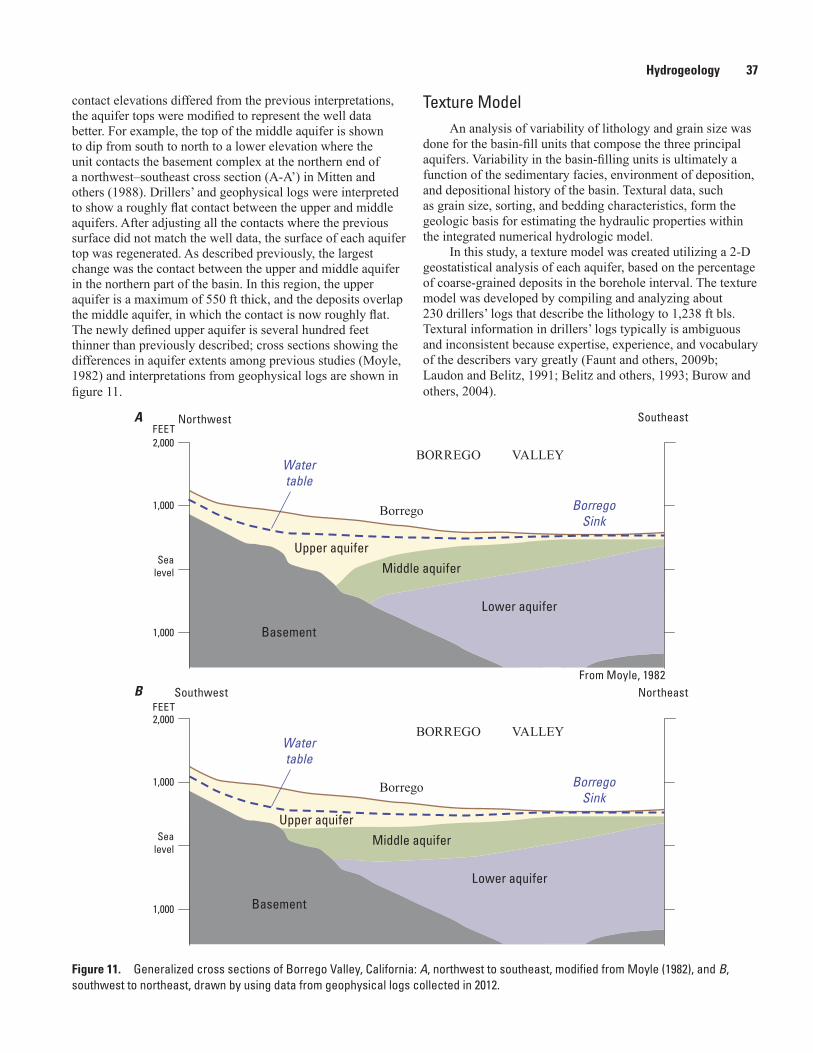
Hydrogeology 37
contact elevations differed from the previous interpretations, the aquifer tops were modified to represent the well data better. For example, the top of the middle aquifer is shown to dip from south to north to a lower elevation where the unit contacts the basement complex at the northern end of a northwest–southeast cross section (A-A’) in Mitten and others (1988). Drillers’ and geophysical logs were interpreted to show a roughly flat contact between the upper and middle aquifers. After adjusting all the contacts where the previous surface did not match the well data, the surface of each aquifer top was regenerated. As described previously, the largest change was the contact between the upper and middle aquifer in the northern part of the basin. In this region, the upper aquifer is a maximum of 550 ft thick, and the deposits overlap the middle aquifer, in which the contact is now roughly flat. The newly defined upper aquifer is several hundred feet thinner than previously described; cross sections showing the differences in aquifer extents among previous studies (Moyle, 1982) and interpretations from geophysical logs are shown in figure 11.
Texture ModelAn analysis of variability of lithology and grain size was
done for the basin-fill units that compose the three principal aquifers. Variability in the basin-filling units is ultimately a function of the sedimentary facies, environment of deposition, and depositional history of the basin. Textural data, such as grain size, sorting, and bedding characteristics, form the geologic basis for estimating the hydraulic properties within the integrated numerical hydrologic model.
In this study, a texture model was created utilizing a 2-D geostatistical analysis of each aquifer, based on the percentage of coarse-grained deposits in the borehole interval. The texture model was developed by compiling and analyzing about 230 drillers’ logs that describe the lithology to 1,238 ft bls. Textural information in drillers’ logs typically is ambiguous and inconsistent because expertise, experience, and vocabulary of the describers vary greatly (Faunt and others, 2009b; Laudon and Belitz, 1991; Belitz and others, 1993; Burow and others, 2004).
Figure 11. Generalized cross sections of Borrego Valley, California: A, northwest to southeast, modified from Moyle (1982), and B, southwest to northeast, drawn by using data from geophysical logs collected in 2012.
2,000
1,000
Sealevel
1,000
FEET
Upper aquiferMiddle aquifer
Lower aquifer
Basement
Upper aquiferMiddle aquifer
Lower aquifer
Basement
Watertable
BorregoSink
BORREGO VALLEY
Borrego
From Moyle, 1982
2,000
1,000
Sealevel
1,000
FEET
Watertable
BorregoSink
BORREGO VALLEY
Borrego
sac13-0509_Figure 11 xsec_change
NortheastSouthwest
Northwest SoutheastA
B
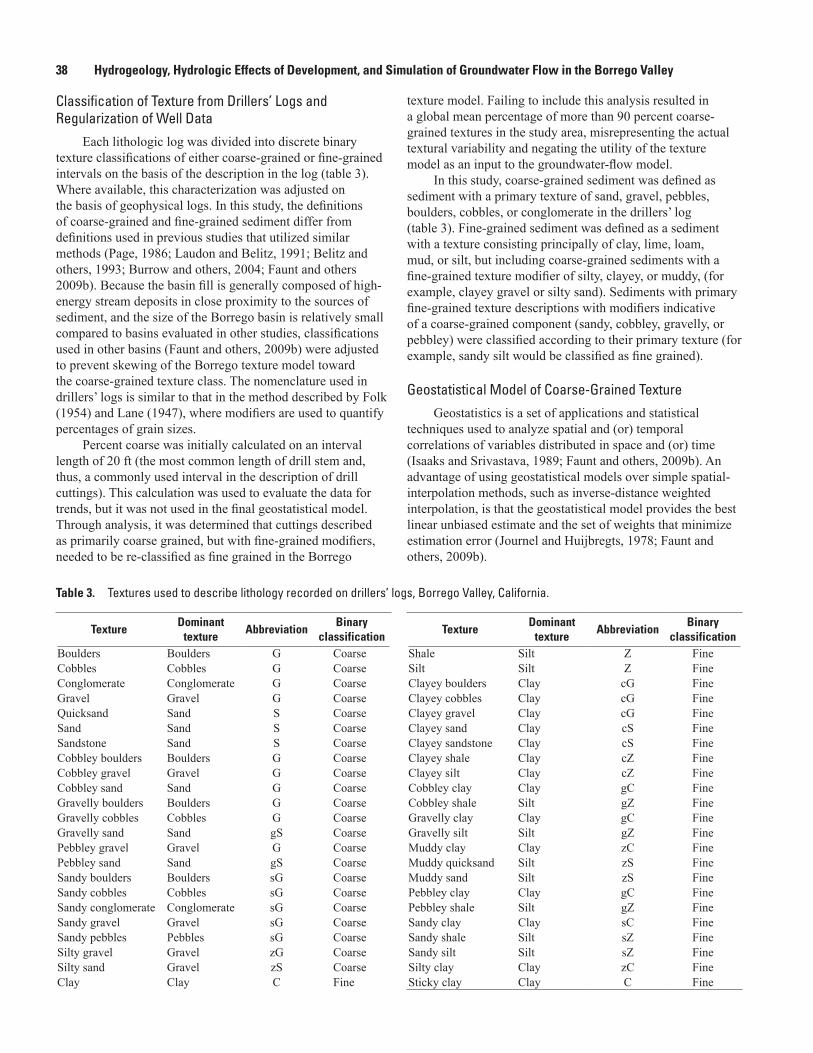
38 Hydrogeology, Hydrologic Effects of Development, and Simulation of Groundwater Flow in the Borrego Valley
Classification of Texture from Drillers’ Logs and Regularization of Well Data
Each lithologic log was divided into discrete binary texture classifications of either coarse-grained or fine-grained intervals on the basis of the description in the log (table 3). Where available, this characterization was adjusted on the basis of geophysical logs. In this study, the definitions of coarse-grained and fine-grained sediment differ from definitions used in previous studies that utilized similar methods (Page, 1986; Laudon and Belitz, 1991; Belitz and others, 1993; Burrow and others, 2004; Faunt and others 2009b). Because the basin fill is generally composed of high-energy stream deposits in close proximity to the sources of sediment, and the size of the Borrego basin is relatively small compared to basins evaluated in other studies, classifications used in other basins (Faunt and others, 2009b) were adjusted to prevent skewing of the Borrego texture model toward the coarse-grained texture class. The nomenclature used in drillers’ logs is similar to that in the method described by Folk (1954) and Lane (1947), where modifiers are used to quantify percentages of grain sizes.
Percent coarse was initially calculated on an interval length of 20 ft (the most common length of drill stem and, thus, a commonly used interval in the description of drill cuttings). This calculation was used to evaluate the data for trends, but it was not used in the final geostatistical model. Through analysis, it was determined that cuttings described as primarily coarse grained, but with fine-grained modifiers, needed to be re-classified as fine grained in the Borrego
texture model. Failing to include this analysis resulted in a global mean percentage of more than 90 percent coarse-grained textures in the study area, misrepresenting the actual textural variability and negating the utility of the texture model as an input to the groundwater-flow model.
In this study, coarse-grained sediment was defined as sediment with a primary texture of sand, gravel, pebbles, boulders, cobbles, or conglomerate in the drillers’ log (table 3). Fine-grained sediment was defined as a sediment with a texture consisting principally of clay, lime, loam, mud, or silt, but including coarse-grained sediments with a fine-grained texture modifier of silty, clayey, or muddy, (for example, clayey gravel or silty sand). Sediments with primary fine-grained texture descriptions with modifiers indicative of a coarse-grained component (sandy, cobbley, gravelly, or pebbley) were classified according to their primary texture (for example, sandy silt would be classified as fine grained).
Geostatistical Model of Coarse-Grained TextureGeostatistics is a set of applications and statistical
techniques used to analyze spatial and (or) temporal correlations of variables distributed in space and (or) time (Isaaks and Srivastava, 1989; Faunt and others, 2009b). An advantage of using geostatistical models over simple spatial-interpolation methods, such as inverse-distance weighted interpolation, is that the geostatistical model provides the best linear unbiased estimate and the set of weights that minimize estimation error (Journel and Huijbregts, 1978; Faunt and others, 2009b).
TextureDominant
textureAbbreviation
Binary classification
Boulders Boulders G CoarseCobbles Cobbles G CoarseConglomerate Conglomerate G CoarseGravel Gravel G CoarseQuicksand Sand S CoarseSand Sand S CoarseSandstone Sand S CoarseCobbley boulders Boulders G CoarseCobbley gravel Gravel G CoarseCobbley sand Sand G CoarseGravelly boulders Boulders G CoarseGravelly cobbles Cobbles G CoarseGravelly sand Sand gS CoarsePebbley gravel Gravel G CoarsePebbley sand Sand gS CoarseSandy boulders Boulders sG CoarseSandy cobbles Cobbles sG CoarseSandy conglomerate Conglomerate sG CoarseSandy gravel Gravel sG CoarseSandy pebbles Pebbles sG CoarseSilty gravel Gravel zG CoarseSilty sand Gravel zS CoarseClay Clay C Fine
TextureDominant
textureAbbreviation
Binary classification
Shale Silt Z FineSilt Silt Z FineClayey boulders Clay cG FineClayey cobbles Clay cG FineClayey gravel Clay cG FineClayey sand Clay cS FineClayey sandstone Clay cS FineClayey shale Clay cZ FineClayey silt Clay cZ FineCobbley clay Clay gC FineCobbley shale Silt gZ FineGravelly clay Clay gC FineGravelly silt Silt gZ FineMuddy clay Clay zC FineMuddy quicksand Silt zS FineMuddy sand Silt zS FinePebbley clay Clay gC FinePebbley shale Silt gZ FineSandy clay Clay sC FineSandy shale Silt sZ FineSandy silt Silt sZ FineSilty clay Clay zC FineSticky clay Clay C Fine
Table 3. Textures used to describe lithology recorded on drillers’ logs, Borrego Valley, California.
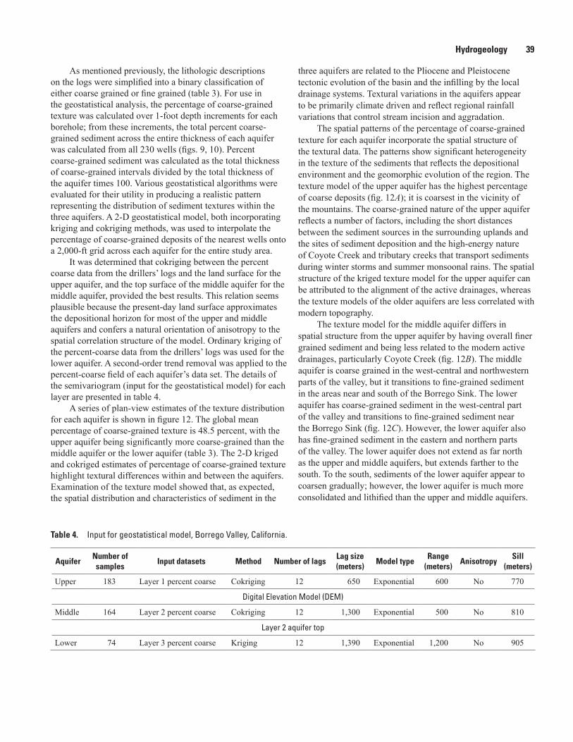
Hydrogeology 39
As mentioned previously, the lithologic descriptions on the logs were simplified into a binary classification of either coarse grained or fine grained (table 3). For use in the geostatistical analysis, the percentage of coarse-grained texture was calculated over 1-foot depth increments for each borehole; from these increments, the total percent coarse-grained sediment across the entire thickness of each aquifer was calculated from all 230 wells (figs. 9, 10). Percent coarse-grained sediment was calculated as the total thickness of coarse-grained intervals divided by the total thickness of the aquifer times 100. Various geostatistical algorithms were evaluated for their utility in producing a realistic pattern representing the distribution of sediment textures within the three aquifers. A 2-D geostatistical model, both incorporating kriging and cokriging methods, was used to interpolate the percentage of coarse-grained deposits of the nearest wells onto a 2,000-ft grid across each aquifer for the entire study area.
It was determined that cokriging between the percent coarse data from the drillers’ logs and the land surface for the upper aquifer, and the top surface of the middle aquifer for the middle aquifer, provided the best results. This relation seems plausible because the present-day land surface approximates the depositional horizon for most of the upper and middle aquifers and confers a natural orientation of anisotropy to the spatial correlation structure of the model. Ordinary kriging of the percent-coarse data from the drillers’ logs was used for the lower aquifer. A second-order trend removal was applied to the percent-coarse field of each aquifer’s data set. The details of the semivariogram (input for the geostatistical model) for each layer are presented in table 4.
A series of plan-view estimates of the texture distribution for each aquifer is shown in figure 12. The global mean percentage of coarse-grained texture is 48.5 percent, with the upper aquifer being significantly more coarse-grained than the middle aquifer or the lower aquifer (table 3). The 2-D kriged and cokriged estimates of percentage of coarse-grained texture highlight textural differences within and between the aquifers. Examination of the texture model showed that, as expected, the spatial distribution and characteristics of sediment in the
three aquifers are related to the Pliocene and Pleistocene tectonic evolution of the basin and the infilling by the local drainage systems. Textural variations in the aquifers appear to be primarily climate driven and reflect regional rainfall variations that control stream incision and aggradation.
The spatial patterns of the percentage of coarse-grained texture for each aquifer incorporate the spatial structure of the textural data. The patterns show significant heterogeneity in the texture of the sediments that reflects the depositional environment and the geomorphic evolution of the region. The texture model of the upper aquifer has the highest percentage of coarse deposits (fig. 12A); it is coarsest in the vicinity of the mountains. The coarse-grained nature of the upper aquifer reflects a number of factors, including the short distances between the sediment sources in the surrounding uplands and the sites of sediment deposition and the high-energy nature of Coyote Creek and tributary creeks that transport sediments during winter storms and summer monsoonal rains. The spatial structure of the kriged texture model for the upper aquifer can be attributed to the alignment of the active drainages, whereas the texture models of the older aquifers are less correlated with modern topography.
The texture model for the middle aquifer differs in spatial structure from the upper aquifer by having overall finer grained sediment and being less related to the modern active drainages, particularly Coyote Creek (fig. 12B). The middle aquifer is coarse grained in the west-central and northwestern parts of the valley, but it transitions to fine-grained sediment in the areas near and south of the Borrego Sink. The lower aquifer has coarse-grained sediment in the west-central part of the valley and transitions to fine-grained sediment near the Borrego Sink (fig. 12C). However, the lower aquifer also has fine-grained sediment in the eastern and northern parts of the valley. The lower aquifer does not extend as far north as the upper and middle aquifers, but extends farther to the south. To the south, sediments of the lower aquifer appear to coarsen gradually; however, the lower aquifer is much more consolidated and lithified than the upper and middle aquifers.
Table 4. Input for geostatistical model, Borrego Valley, California.
AquiferNumber of samples
Input datasets Method Number of lagsLag size(meters)
Model typeRange
(meters)Anisotropy
Sill(meters)
Upper 183 Layer 1 percent coarse Cokriging 12 650 Exponential 600 No 770
Digital Elevation Model (DEM)
Middle 164 Layer 2 percent coarse Cokriging 12 1,300 Exponential 500 No 810
Layer 2 aquifer top
Lower 74 Layer 3 percent coarse Kriging 12 1,390 Exponential 1,200 No 905
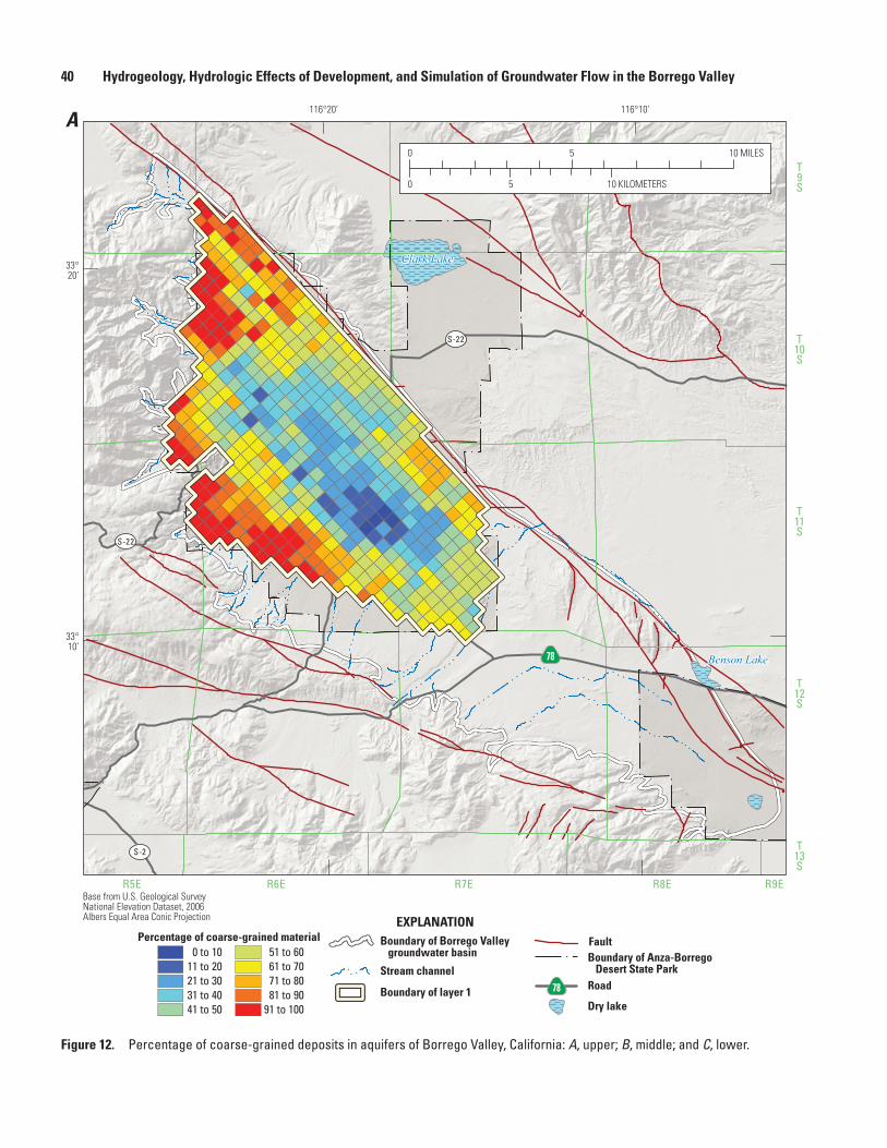
40 Hydrogeology, Hydrologic Effects of Development, and Simulation of Groundwater Flow in the Borrego Valley
Clark Lake
Benson Lake
T9S
T10S
T11S
T12S
T13S
R5E R6E R7E R8E R9EBase from U.S. Geological Survey National Elevation Dataset, 2006Albers Equal Area Conic Projection
S-22
S-22
S-2
78
116°10’116°20’
33°20’
33°10’
sac13-0509_Figure 12a_Percent coarse_upper
A
EXPLANATION
0
0 5 10
5 10 MILES
KILOMETERS
0 to 1011 to 2021 to 3031 to 4041 to 50
51 to 6061 to 7071 to 8081 to 90
91 to 100
Percentage of coarse-grained material
Boundary of layer 1
Stream channel
Boundary of Borrego Valley groundwater basin Boundary of Anza-Borrego
Desert State Park
Fault
Road78
Dry lake
Figure 12. Percentage of coarse-grained deposits in aquifers of Borrego Valley, California: A, upper; B, middle; and C, lower.
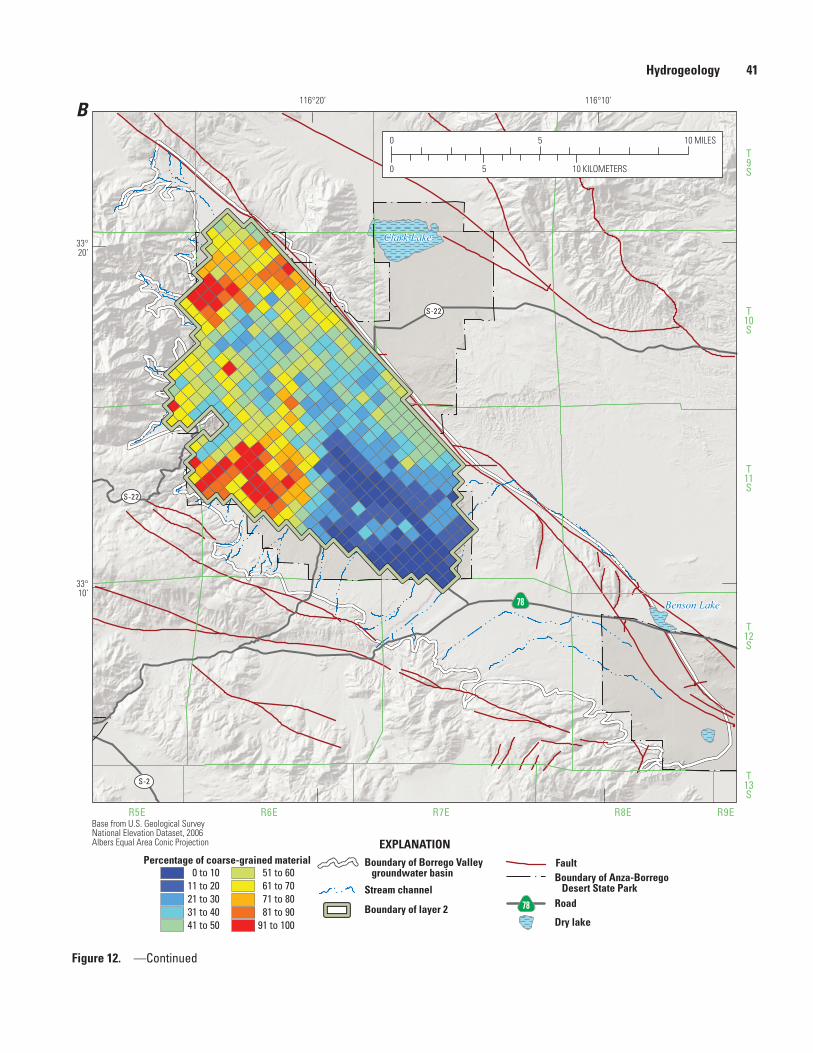
Hydrogeology 41
Clark Lake
BorregoSink
Benson Lake
T9S
T10S
T11S
T12S
T13S
R5E R6E R7E R8E R9EBase from U.S. Geological Survey National Elevation Dataset, 2006Albers Equal Area Conic Projection
S-22
S-22
S-2
78
116°10’116°20’
33°20’
33°10’
sac13-0509_Figure 12b_Percent coarse_middle
B
EXPLANATION
0 to 1011 to 2021 to 3031 to 4041 to 50
51 to 6061 to 7071 to 8081 to 90
91 to 100
Percentage of coarse-grained material
Boundary of layer 2
Stream channel
Boundary of Borrego Valley groundwater basin
0
0 5 10
5 10 MILES
KILOMETERS
Boundary of Anza-Borrego Desert State Park
Fault
Road78
Dry lake
Figure 12. —Continued
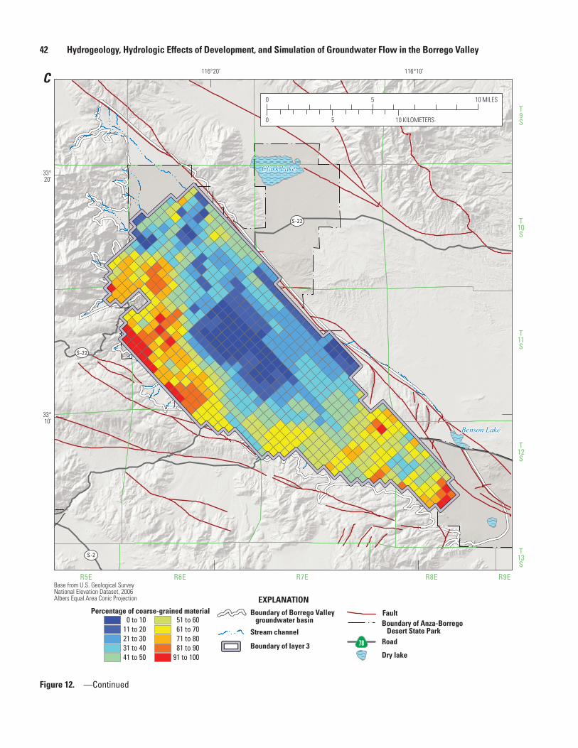
42 Hydrogeology, Hydrologic Effects of Development, and Simulation of Groundwater Flow in the Borrego Valley
Clark Lake
BorregoSink
Benson Lake
T9S
T10S
T11S
T12S
T13S
R5E R6E R7E R8E R9EBase from U.S. Geological Survey National Elevation Dataset, 2006Albers Equal Area Conic Projection
S-22
S-22
S-2
78
116°10’116°20’
33°20’
33°10’
sac13-0509_Figure 12c_Percent coarse_lower
C0
0 5 10
5 10 MILES
KILOMETERS
EXPLANATION
0 to 1011 to 2021 to 3031 to 4041 to 50
51 to 6061 to 7071 to 8081 to 90
91 to 100
Percentage of coarse-grained material
Boundary of layer 3
Stream channel
Boundary of Borrego Valley groundwater basin Boundary of Anza-Borrego
Desert State Park
Fault
Road78
Dry lake
Figure 12. —Continued
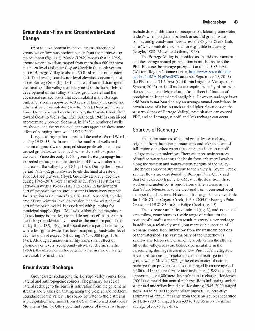
Hydrogeology 43
Groundwater-Flow and Groundwater-Level Change
Prior to development in the valley, the direction of groundwater flow was predominantly from the northwest to the southeast (fig. 13A). Moyle (1982) reports that in 1945, groundwater elevations ranged from more than 600 ft above mean sea level (asl) near Coyote Creek in the northwestern part of Borrego Valley to about 460 ft asl in the southeastern part. The lowest groundwater-level elevations occurred east of the Borrego Sink (fig. 13A), an area of natural drainage in the middle of the valley that is dry most of the time. Before development of the valley, shallow groundwater and the occasional surface water that accumulated in the Borrego Sink after storms supported 450 acres of honey mesquite and other native phreatophytes (Moyle, 1982). Deep groundwater flowed to the east and southeast along the Coyote Creek fault toward Ocotillo Wells (fig. 13A). Although 1945 is considered approximately pre-development, in 1945, a number of wells are shown, and the water-level contours appear to show some effect of pumping from well 11S/7E-20P1.
Large-scale agriculture predated the end of World War II, and by 1952–53, the increase in the number of wells and amount of groundwater pumped since predevelopment had caused groundwater-level declines in the northern part of the basin. Since the early 1950s, groundwater pumpage has exceeded recharge, and the direction of flow was altered in all areas of the valley by 2010 (fig. 13B). During the 11 year period 1952–62, groundwater levels declined at a rate of about 3.4 feet per year (ft/yr). Groundwater-level declines during 1945–2010 were as much as 2.1 ft/yr (119 ft for the period) in wells 10S/6E-21A1 and -21A2 in the northern part of the basin, where groundwater is intensively pumped for irrigation agriculture (figs. 13B, 14A). A second, smaller area of groundwater-level depression is in the west-central part of the basin, which is associated with pumping for municipal supply (figs. 13B, 14B). Although the magnitude of the change is smaller, the middle portion of the basin has a similar groundwater-level trend as the northern part of the valley (figs. 13B, 14C). In the southeastern part of the valley, where less groundwater has been pumped, groundwater-level declines did not exceed 6 ft during 1945–2008 (figs. 13B, 14D). Although climate variability has a small effect on groundwater levels (see groundwater-level declines in the 1950s), the effects of anthropogenic water use far outweigh the variability in climate.
Groundwater Recharge
Groundwater recharge to the Borrego Valley comes from natural and anthropogenic sources. The primary source of natural recharge to the basin is infiltration from the ephemeral streams and washes emanating along the western and northern boundaries of the valley. The source of water to these streams is precipitation and runoff from the San Ysidro and Santa Rosa Mountains (fig. 1). Other potential sources of natural recharge
include direct infiltration of precipitation, lateral groundwater underflow from adjacent bedrock areas and groundwater basins, and groundwater flow across the Coyote Creek fault, all of which probably are small or negligible in quantity (Moyle, 1982; Mitten and others, 1988).
The Borrego Valley is classified as an arid environment, and the average annual precipitation is much less than the PET. Because the average precipitation rate is 5.83 in/yr. (Western Region Climate Center, http://www.wrcc.dri.edu/cgi-bin/cliMAIN.pl?ca0983 accessed September 29, 2015), the PET rate is 71.6 in/yr (California Irrigation Management System, 2012), and soil moisture requirements by plants near the root zone are high, recharge from direct infiltration of precipitation is considered negligible. However, recharge in an arid basin is not based solely on average annual conditions. In certain areas of a basin (such as the higher elevations on the western slopes of Borrego Valley), precipitation can exceed PET, and soil storage, runoff, and (or) recharge can occur.
Sources of Recharge
The major sources of natural groundwater recharge originate from the adjacent mountains and take the form of infiltration of surface water that enters the basin as runoff and groundwater underflow. There are three main sources of surface water that enter the basin from ephemeral washes along the western and southwestern margins of the valley. The major source of streamflow to the valley is Coyote Creek; smaller flows are contributed by Borrego Palm Creek and San Felipe Creek (figs. 1, 15). Most of the flow from these washes and underflow is runoff from winter storms in the San Ysidro Mountains to the west and from occasional local summer thunderstorms. Historical discharge data are available for 1950–83 for Coyote Creek, 1950–2004 for Borrego Palm Creek, and 1958–83 for San Felipe Creek (fig. 15).
The extreme variability of rainfall (fig. 3), and associated streamflow, contributes to a wide range of values for the portion of runoff estimated to result in groundwater recharge. In addition, a relatively small, but more stable, portion of recharge comes from underflow from the upstream portions of the watershed. The vast majority of the underflow is shallow and follows the channel network within the alluvial fill of the valleys because bedrock permeability in the surrounding drainage areas is so low. Previous investigators have used various approaches to estimate recharge to the groundwater. Moyle (1982) gathered estimates of natural recharge from previous studies that ranged from averages of 3,300 to 11,000 acre-ft/yr. Mitten and others (1988) estimated approximately 4,800 acre-ft/yr of natural recharge. Henderson (2001) estimated that annual recharge from infiltrating surface water and underflow into the valley during 1945–2000 ranged from 760 to 51,000 acre-ft and averaged 6,170 acre-ft/yr. Estimates of annual recharge from the same sources identified by Netto (2001) ranged from 633 to 45,935 acre-ft with an average of 5,670 acre-ft/yr.
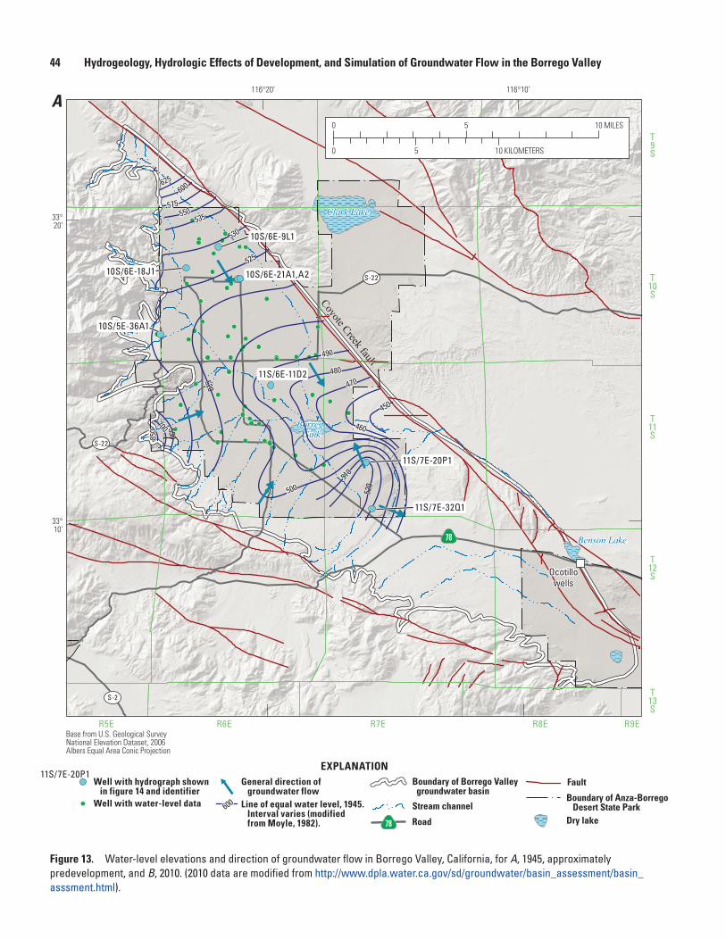
44 Hydrogeology, Hydrologic Effects of Development, and Simulation of Groundwater Flow in the Borrego Valley
Figure 13. Water-level elevations and direction of groundwater flow in Borrego Valley, California, for A, 1945, approximately predevelopment, and B, 2010. (2010 data are modified from http://www.dpla.water.ca.gov/sd/groundwater/basin_assessment/basin_asssment.html).
Coyote Creek fault
Clark Lake
BorregoSink
Benson Lake
T9S
T10S
T11S
T12S
T13S
R5E R6E R7E R8E R9EBase from U.S. Geological Survey National Elevation Dataset, 2006Albers Equal Area Conic Projection
S-22
S-22
S-2
78
10S/5E-36A1
10S/6E-9L1
10S/6E-21A1,A210S/6E-18J1
Ocotillowells
500
520
490
480
525
530
470
535
460
510
550575
600
450
700
625
850
520
530
116°10’116°20’
33°20’
33°10’
sac13-0509_Figure 13a 1945 WL contours
A
EXPLANATION
0
0 5 10
5 10 MILES
KILOMETERS
Well with hydrograph shown in figure 14 and identifierWell with water-level data
11S/7E-20P1
Line of equal water level, 1945. Interval varies (modified from Moyle, 1982).
General direction of groundwater flow
Stream channel
Boundary of Borrego Valley groundwater basin
Boundary of Anza-Borrego Desert State Park
Fault
600
Road78
11S/6E-11D2
11S/7E-20P1
11S/7E-32Q1
Dry lake
Hydrogeology 45
Figure 13. —Continued
Coyote Creek fault
Clark Lake
BorregoSink
Benson Lake
T9S
T10S
T11S
T12S
T13S
R5E R6E R7E R8E R9E
S-22
S-22
S-2
78
l
l
420
410
480
430440
400
500
460
470
450
390
380 340360 420
400
420
410
440
460
380
430
390
11S/7E-20P1
11S/7E-32Q1
10S/5E-36A1
10S/6E-9L1
10S/6E-21A1,A2
11S/6E-11D2
10S/6E-18J1
116°10’116°20’
33°20’
33°10’
0
0 5 10
5 10 MILES
KILOMETERS
sac13-0509_Figure 13b 2010 WL Contours
B
EXPLANATION
Well with hydrograph shown in figure 14 and identifierWell with water-level data
11S/7E-20P1
Line of equal water level, 2010. Interval varies; hatchures indicate depression
General direction of groundwater flow
Stream channel
Boundary of Borrego Valley groundwater basin
600
Road78
Base from U.S. Geological Survey National Elevation Dataset, 2006Albers Equal Area Conic Projection
Boundary of Anza-Borrego Desert State Park
Fault
Dry lake
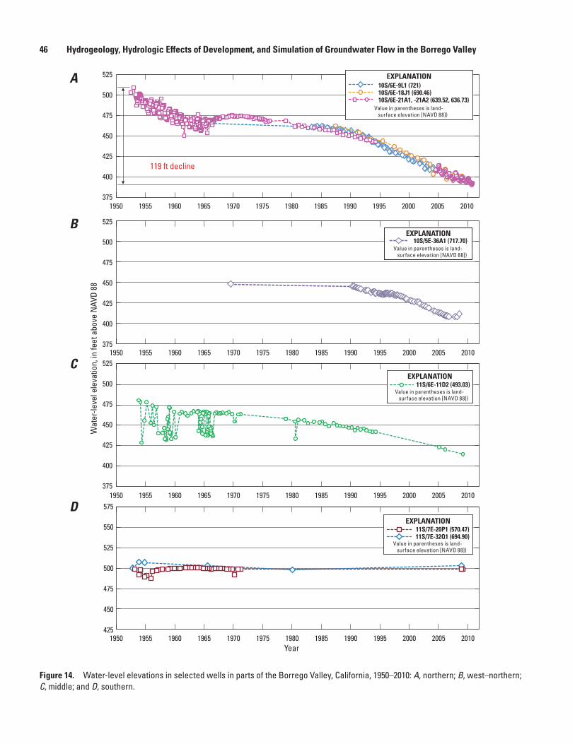
46 Hydrogeology, Hydrologic Effects of Development, and Simulation of Groundwater Flow in the Borrego Valley
Figure 14. Water-level elevations in selected wells in parts of the Borrego Valley, California, 1950–2010: A, northern; B, west–northern; C, middle; and D, southern.
119 ft decline
375
400
425
450
475
500
525
375
400
425
450
475
500
525
375
400
425
450
475
500
525
1950 1955 1960 1965 1970 1975 1980 1985 1990 1995 2000 2005 2010
1950 1955 1960 1965 1970 1975 1980 1985 1990 1995 2000 2005 2010
Year
A
B
1950 1955 1960 1965 1970 1975 1980 1985 1990 1995 2000 2005 2010
Wat
er-le
vel e
leva
tion,
in fe
et a
bove
NAV
D 88
C
425
450
475
500
525
550
575
1950 1955 1960 1965 1970 1975 1980 1985 1990 1995 2000 2005 2010
D
sac13-0509_Figure 14 hydros
10S/6E-9L1 (721)10S/6E-18J1 (690.46)10S/6E-21A1, -21A2 (639.52, 636.73)
EXPLANATION
Value in parentheses is land-surface elevation [NAVD 88])
10S/5E-36A1 (717.70)EXPLANATION
Value in parentheses is land-surface elevation [NAVD 88])
11S/6E-11D2 (493.03)EXPLANATION
Value in parentheses is land-surface elevation [NAVD 88])
11S/7E-32Q1 (694.90)11S/7E-20P1 (570.47)
EXPLANATION
Value in parentheses is land-surface elevation [NAVD 88])
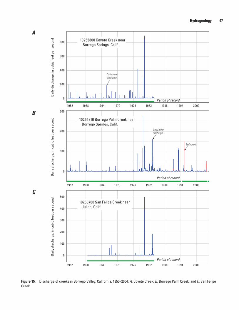
Hydrogeology 47
Figure 15. Discharge of creeks in Borrego Valley, California, 1950–2004: A, Coyote Creek; B, Borrego Palm Creek; and C, San Felipe Creek.
sac13-0509_Figure 15abc_daily discharge
0
200
400
600
800
Daily
dis
char
ge, i
n cu
bic
feet
per
sec
ond
1952 1958 1964 1970 1976 1982 1988 1994 2000
10255800 Coyote Creek near Borrego Springs, Calif.
Period of record
0
100
200
300
Daily
dis
char
ge, i
n cu
bic
feet
per
sec
ond
1952 1958 1964 1970 1976 1982 1988 1994 2000
10255810 Borrego Palm Creek near Borrego Springs, Calif.
10255700 San Felipe Creek near Julian, Calif.
Period of record
0
100
200
400
300
500
Daily
dis
char
ge, i
n cu
bic
feet
per
sec
ond
1952 1958 1964 1970 1976 1982 1988 1994 2000
Period of record
A
B
C
Estimated
Daily meandischarge
Daily meandischarge

48 Hydrogeology, Hydrologic Effects of Development, and Simulation of Groundwater Flow in the Borrego Valley
New anthropogenic sources of recharge accompanied development in the basin, including irrigation-return flow from agricultural fields and municipal lawns and the infiltration of treated wastewater and untreated wastewater from septic systems. From the late 1940s onward, these sources of anthropogenic recharge have significantly increased the total groundwater recharge in the valley, at times becoming many times larger in magnitude than natural recharge. On the basis of a chloride mass-balance technique, Netto (2001) estimated irrigation return flow to the groundwater system at a citrus grove and a golf course fairway to be 22 percent and 14 percent, respectively. Any water from these anthropogenic sources that reaches the water table by infiltrating the vadose zone is part of the overall water budget. This water is a component of recharge in the integrated hydrologic model (described in the “Integrated Hydrologic Model” section of this report).
Transient Estimates of Natural Recharge from the Basin Characterization Model
As mentioned previously, estimates of the quantity, distribution, and source of natural groundwater recharge vary widely. Therefore, the regional-scale Basin Characterization Model (BCM; Flint and others, 2004) was used to better quantify components of the natural groundwater recharge (underflow and streamflow into the Borrego Valley). The BCM uses a deterministic water-balance approach to estimate recharge and runoff in a basin. The model uses the distribution of precipitation, snow accumulation and melt, PET, soil-water storage, and bedrock permeability to estimate a monthly water balance for the groundwater system. Results from the BCM are useful for providing bounds associated with water-balance results of more detailed models, evaluating long-term climate conditions, illustrating the mechanisms responsible for recharge in a basin, and comparing the locations and volumes of recharge and runoff in different basins on a regional scale (Flint and Martin, 2012).
The BCM is grid based at a spatial resolution of 886 ft (270 m) and calculates monthly recharge and runoff. The BCM incorporates spatially distributed parameters (monthly precipitation, monthly minimum and maximum air temperature, monthly PET, soil-water storage capacity, and saturated vertical hydraulic conductivity (K) of bedrock and alluvium) to determine where excess water is available in a basin and whether the excess water is stored in the soil or infiltrates downward into underlying bedrock. Excess water is partitioned by the BCM as either potential in-place recharge or potential runoff, depending on the saturated K of bedrock and alluvium. Potential in-place recharge is the maximum volume of water for a given month that can recharge directly into bedrock or deep alluvium (greater than 20 ft). Potential runoff is the maximum volume of water for a given month
that runs off the mountain front or becomes streamflow. The total of runoff and underflow from upstream components of the watershed is the summation of in-place recharge and a percentage of runoff that is determined through calibration to measured streamflow (Flint and Flint, 2007a). The downscaled PRISM precipitation and air-temperature maps were used with the monthly PET results (fig. 4), available spatial maps of elevation, bedrock permeability estimated from the geology (fig. 7), and soil-water storage from the State Soil Geographic Data Base (STATSGO; National Resources Conservation Service, 2006) to calculate snow accumulation and melt snow and to calculate changes in soil moisture, runoff, and recharge.
The BCM calculates potential in-place recharge and potential runoff and generates distributions of both components. In this study, the BCM provided estimates of the underflow from the adjacent mountains and basins and potential runoff in stream channels into the basin. Moreover, the BCM can be used to compare the potential for recharge under the current climate (2010) and that for past wetter and drier climates (Flint and Flint, 2007a). The BCM model domain includes the watersheds that surround and drain into the Borrego Valley (fig. 16).
PET and snow modules of the BCM were calibrated regionally throughout the southwestern United States to measured PET data and the Moderate-Resolution Imaging Spectroradiometer (MODIS) snow-cover data (U.S. Geological Survey, 2007; Flint and Flint, 2007b). For this study, the model was also calibrated to measured unimpaired streamflow data. The determination of whether excess water becomes recharge or runoff is governed in part by the underlying bedrock characteristics that govern permeability (fig. 16). The greater the bedrock permeability, the greater the recharge and the less the runoff generated for a given grid cell. In small, gaged watersheds that generate unimpaired flows, the bedrock permeability can be adjusted to calculate a total watershed discharge that matches the measured watershed discharge. Following calibration to bedrock permeability, recharge and runoff can be accumulated for all grid cells upstream from streamgages to account for stream channel gains and losses to calculate basin discharge and optimize the fit between total measured volume and simulated volume for the period of record for each gage. The simple exponential equations described in detail in Flint and others (2013) were used to calculate surface-water flow recession, seepage, and base flow that can extend throughout the dry season; constrain estimates of flow and recharge when measured data are not available; and provide estimates of flows and recharge in ungaged basins. In the Borrego Valley region, there are three streamgages that represent unimpaired flows, which were used for model calibration (figs. 15, 16). However, two of the streamgages (10255800 and 10255700) are downstream from large alluvial valleys in which an unknown amount of runoff that reaches the streams infiltrates the streambeds and potentially recharges the local water table.
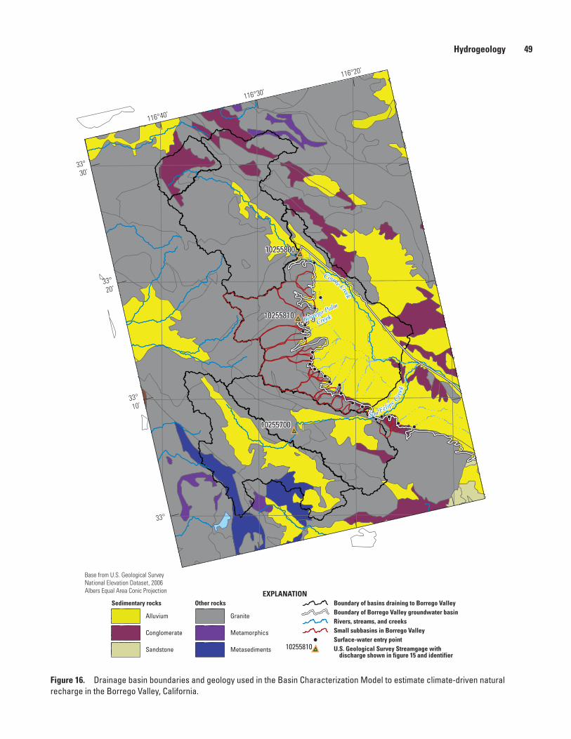
Hydrogeology 49
Figure 16. Drainage basin boundaries and geology used in the Basin Characterization Model to estimate climate-driven natural recharge in the Borrego Valley, California.
sac13-0509_figure 16_BCM_updated
116°20’
116°30’
116°40’
33°30’
33°20’
33°10’
33°
EXPLANATION
10255810
10255800
10255700
Alluvium
Conglomerate
Granite
Metamorphics
MetasedimentsSandstoneSurface-water entry point
Boundary of basins draining to Borrego ValleySedimentary rocks Other rocks
Rivers, streams, and creeksSmall subbasins in Borrego Valley
Boundary of Borrego Valley groundwater basin
U.S. Geological Survey Streamgage with discharge shown in figure 15 and identifier
10255810
Borrego Palm
Creek
Coyote Creek
San Felip
e Cre
ek
Base from U.S. Geological Survey National Elevation Dataset, 2006Albers Equal Area Conic Projection
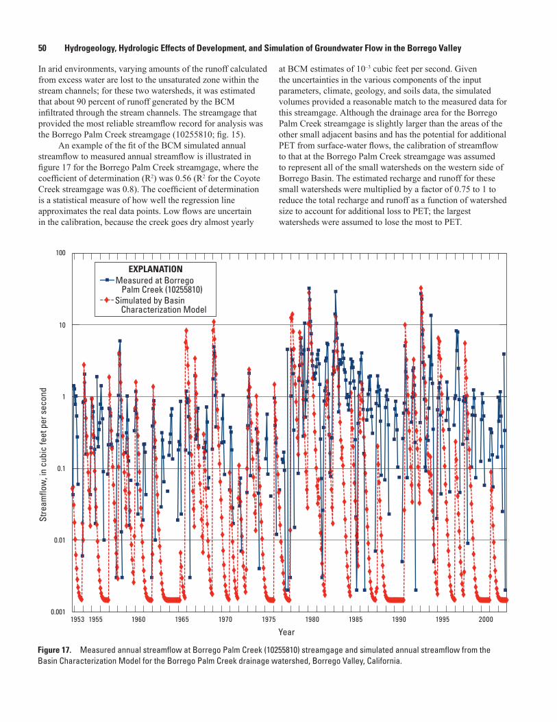
50 Hydrogeology, Hydrologic Effects of Development, and Simulation of Groundwater Flow in the Borrego Valley
In arid environments, varying amounts of the runoff calculated from excess water are lost to the unsaturated zone within the stream channels; for these two watersheds, it was estimated that about 90 percent of runoff generated by the BCM infiltrated through the stream channels. The streamgage that provided the most reliable streamflow record for analysis was the Borrego Palm Creek streamgage (10255810; fig. 15).
An example of the fit of the BCM simulated annual streamflow to measured annual streamflow is illustrated in figure 17 for the Borrego Palm Creek streamgage, where the coefficient of determination (R2) was 0.56 (R2 for the Coyote Creek streamgage was 0.8). The coefficient of determination is a statistical measure of how well the regression line approximates the real data points. Low flows are uncertain in the calibration, because the creek goes dry almost yearly
at BCM estimates of 10–3 cubic feet per second. Given the uncertainties in the various components of the input parameters, climate, geology, and soils data, the simulated volumes provided a reasonable match to the measured data for this streamgage. Although the drainage area for the Borrego Palm Creek streamgage is slightly larger than the areas of the other small adjacent basins and has the potential for additional PET from surface-water flows, the calibration of streamflow to that at the Borrego Palm Creek streamgage was assumed to represent all of the small watersheds on the western side of Borrego Basin. The estimated recharge and runoff for these small watersheds were multiplied by a factor of 0.75 to 1 to reduce the total recharge and runoff as a function of watershed size to account for additional loss to PET; the largest watersheds were assumed to lose the most to PET.
Figure 17. Measured annual streamflow at Borrego Palm Creek (10255810) streamgage and simulated annual streamflow from the Basin Characterization Model for the Borrego Palm Creek drainage watershed, Borrego Valley, California.
sac13-0509_Figure 17 basin discharge
0.001
0.01
0.1
1
10
100
Stre
amflo
w, i
n cu
bic
feet
per
sec
ond
Measured at Borrego Palm Creek (10255810)
EXPLANATION
Simulated by Basin Characterization Model
Year1953 1955 1960 1965 1970 1975 1980 1985 1990 1995 2000
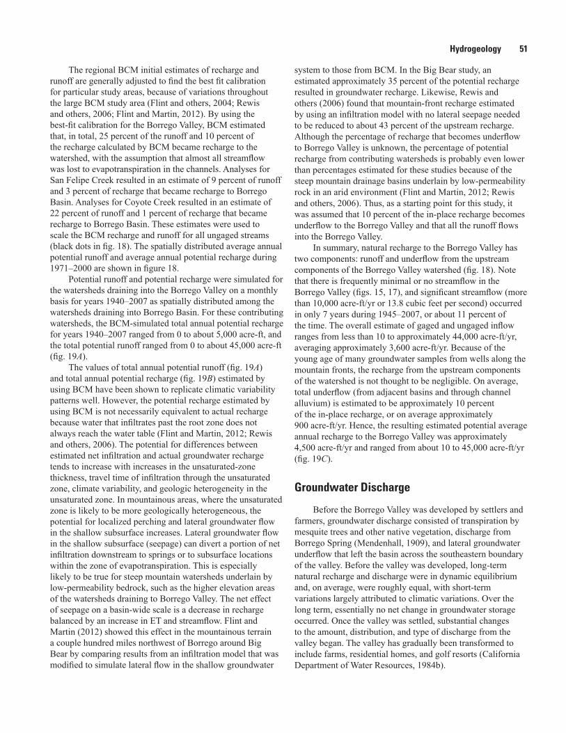
Hydrogeology 51
The regional BCM initial estimates of recharge and runoff are generally adjusted to find the best fit calibration for particular study areas, because of variations throughout the large BCM study area (Flint and others, 2004; Rewis and others, 2006; Flint and Martin, 2012). By using the best-fit calibration for the Borrego Valley, BCM estimated that, in total, 25 percent of the runoff and 10 percent of the recharge calculated by BCM became recharge to the watershed, with the assumption that almost all streamflow was lost to evapotranspiration in the channels. Analyses for San Felipe Creek resulted in an estimate of 9 percent of runoff and 3 percent of recharge that became recharge to Borrego Basin. Analyses for Coyote Creek resulted in an estimate of 22 percent of runoff and 1 percent of recharge that became recharge to Borrego Basin. These estimates were used to scale the BCM recharge and runoff for all ungaged streams (black dots in fig. 18). The spatially distributed average annual potential runoff and average annual potential recharge during 1971–2000 are shown in figure 18.
Potential runoff and potential recharge were simulated for the watersheds draining into the Borrego Valley on a monthly basis for years 1940–2007 as spatially distributed among the watersheds draining into Borrego Basin. For these contributing watersheds, the BCM-simulated total annual potential recharge for years 1940–2007 ranged from 0 to about 5,000 acre-ft, and the total potential runoff ranged from 0 to about 45,000 acre-ft (fig. 19A).
The values of total annual potential runoff (fig. 19A) and total annual potential recharge (fig. 19B) estimated by using BCM have been shown to replicate climatic variability patterns well. However, the potential recharge estimated by using BCM is not necessarily equivalent to actual recharge because water that infiltrates past the root zone does not always reach the water table (Flint and Martin, 2012; Rewis and others, 2006). The potential for differences between estimated net infiltration and actual groundwater recharge tends to increase with increases in the unsaturated-zone thickness, travel time of infiltration through the unsaturated zone, climate variability, and geologic heterogeneity in the unsaturated zone. In mountainous areas, where the unsaturated zone is likely to be more geologically heterogeneous, the potential for localized perching and lateral groundwater flow in the shallow subsurface increases. Lateral groundwater flow in the shallow subsurface (seepage) can divert a portion of net infiltration downstream to springs or to subsurface locations within the zone of evapotranspiration. This is especially likely to be true for steep mountain watersheds underlain by low-permeability bedrock, such as the higher elevation areas of the watersheds draining to Borrego Valley. The net effect of seepage on a basin-wide scale is a decrease in recharge balanced by an increase in ET and streamflow. Flint and Martin (2012) showed this effect in the mountainous terrain a couple hundred miles northwest of Borrego around Big Bear by comparing results from an infiltration model that was modified to simulate lateral flow in the shallow groundwater
system to those from BCM. In the Big Bear study, an estimated approximately 35 percent of the potential recharge resulted in groundwater recharge. Likewise, Rewis and others (2006) found that mountain-front recharge estimated by using an infiltration model with no lateral seepage needed to be reduced to about 43 percent of the upstream recharge. Although the percentage of recharge that becomes underflow to Borrego Valley is unknown, the percentage of potential recharge from contributing watersheds is probably even lower than percentages estimated for these studies because of the steep mountain drainage basins underlain by low-permeability rock in an arid environment (Flint and Martin, 2012; Rewis and others, 2006). Thus, as a starting point for this study, it was assumed that 10 percent of the in-place recharge becomes underflow to the Borrego Valley and that all the runoff flows into the Borrego Valley.
In summary, natural recharge to the Borrego Valley has two components: runoff and underflow from the upstream components of the Borrego Valley watershed (fig. 18). Note that there is frequently minimal or no streamflow in the Borrego Valley (figs. 15, 17), and significant streamflow (more than 10,000 acre-ft/yr or 13.8 cubic feet per second) occurred in only 7 years during 1945–2007, or about 11 percent of the time. The overall estimate of gaged and ungaged inflow ranges from less than 10 to approximately 44,000 acre-ft/yr, averaging approximately 3,600 acre-ft/yr. Because of the young age of many groundwater samples from wells along the mountain fronts, the recharge from the upstream components of the watershed is not thought to be negligible. On average, total underflow (from adjacent basins and through channel alluvium) is estimated to be approximately 10 percent of the in-place recharge, or on average approximately 900 acre-ft/yr. Hence, the resulting estimated potential average annual recharge to the Borrego Valley was approximately 4,500 acre-ft/yr and ranged from about 10 to 45,000 acre-ft/yr (fig. 19C).
Groundwater Discharge
Before the Borrego Valley was developed by settlers and farmers, groundwater discharge consisted of transpiration by mesquite trees and other native vegetation, discharge from Borrego Spring (Mendenhall, 1909), and lateral groundwater underflow that left the basin across the southeastern boundary of the valley. Before the valley was developed, long-term natural recharge and discharge were in dynamic equilibrium and, on average, were roughly equal, with short-term variations largely attributed to climatic variations. Over the long term, essentially no net change in groundwater storage occurred. Once the valley was settled, substantial changes to the amount, distribution, and type of discharge from the valley began. The valley has gradually been transformed to include farms, residential homes, and golf resorts (California Department of Water Resources, 1984b).
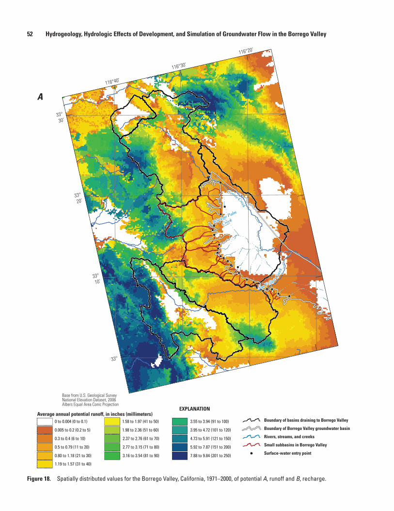
52 Hydrogeology, Hydrologic Effects of Development, and Simulation of Groundwater Flow in the Borrego Valley
sac13-0509_figure 18a_runoff_updated
116°20’
116°30’
116°40’
33°30’
33°20’
33°10’
33°
EXPLANATIONAverage annual potential runoff, in inches (millimeters)
3.16 to 3.54 (81 to 90) 7.88 to 9.84 (201 to 250)0.80 to 1.18 (21 to 30)
1.19 to 1.57 (31 to 40)
3.55 to 3.94 (91 to 100)0 to 0.004 (0 to 0.1) 1.58 to 1.97 (41 to 50)
3.95 to 4.72 (101 to 120)0.005 to 0.2 (0.2 to 5) 1.98 to 2.36 (51 to 60)
4.73 to 5.91 (121 to 150)0.3 to 0.4 (6 to 10) 2.37 to 2.76 (61 to 70)
5.92 to 7.87 (151 to 200)0.5 to 0.79 (11 to 20) 2.77 to 3.15 (71 to 80)Surface-water entry point
Boundary of basins draining to Borrego Valley
Rivers, streams, and creeks
Small subbasins in Borrego Valley
Boundary of Borrego Valley groundwater basin
Borrego Palm
Creek
Coyote Creek
San Felip
e Cre
ek
Base from U.S. Geological Survey National Elevation Dataset, 2006Albers Equal Area Conic Projection
A
Figure 18. Spatially distributed values for the Borrego Valley, California, 1971–2000, of potential A, runoff and B, recharge.
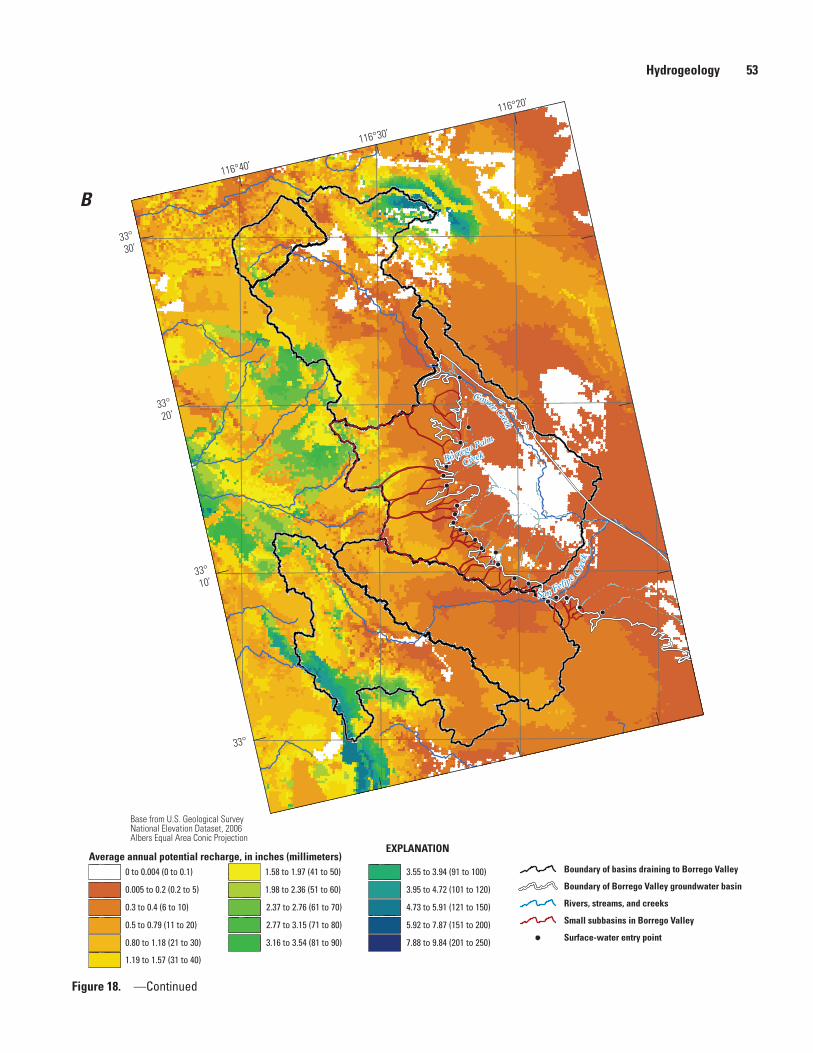
Hydrogeology 53
sac13-0509_figure 18b_recharge_updated
116°20’
116°30’
116°40’
33°30’
33°20’
33°10’
33°
EXPLANATIONAverage annual potential recharge, in inches (millimeters)
3.16 to 3.54 (81 to 90) 7.88 to 9.84 (201 to 250)0.80 to 1.18 (21 to 30)
1.19 to 1.57 (31 to 40)
3.55 to 3.94 (91 to 100)0 to 0.004 (0 to 0.1) 1.58 to 1.97 (41 to 50)
3.95 to 4.72 (101 to 120)0.005 to 0.2 (0.2 to 5) 1.98 to 2.36 (51 to 60)
4.73 to 5.91 (121 to 150)0.3 to 0.4 (6 to 10) 2.37 to 2.76 (61 to 70)
5.92 to 7.87 (151 to 200)0.5 to 0.79 (11 to 20) 2.77 to 3.15 (71 to 80)Surface-water entry point
Boundary of basins draining to Borrego Valley
Rivers, streams, and creeks
Small subbasins in Borrego Valley
Boundary of Borrego Valley groundwater basin
Borrego Palm
Creek
Coyote Creek
San Felipe C
reek
Base from U.S. Geological Survey National Elevation Dataset, 2006Albers Equal Area Conic Projection
B
Figure 18. —Continued
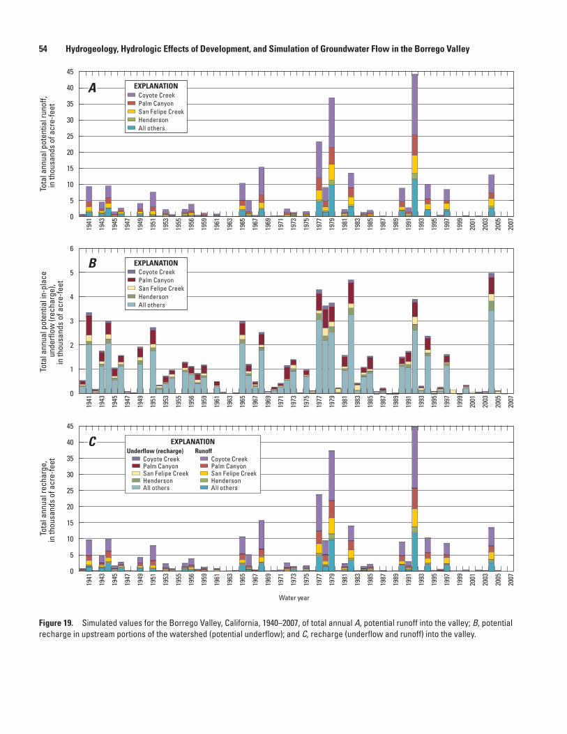
54 Hydrogeology, Hydrologic Effects of Development, and Simulation of Groundwater Flow in the Borrego Valley
Figure 19. Simulated values for the Borrego Valley, California, 1940–2007, of total annual A, potential runoff into the valley; B, potential recharge in upstream portions of the watershed (potential underflow); and C, recharge (underflow and runoff) into the valley.
0
1
2
3
4
5
6
Tota
l ann
ual p
oten
tial i
n-pl
ace
unde
rflow
(rec
harg
e),
in th
ousa
nds
of a
cre-
feet
Water year
0
10
15
5
20
25
30
35
45
40
1941
1943
1945
1947
1949
1951
1953
1955
1956
1959
1961
1963
1965
1967
1969
1971
1973
1975
1977
1979
1981
1983
1985
1987
1989
1991
1993
1995
1997
1999
2001
2003
2005
2007
1941
1943
1945
1947
1949
1951
1953
1955
1956
1959
1961
1963
1965
1967
1969
1971
1973
1975
1977
1979
1981
1983
1985
1987
1989
1991
1993
1995
1997
1999
2001
2003
2005
2007
1941
1943
1945
1947
1949
1951
1953
1955
1956
1959
1961
1963
1965
1967
1969
1971
1973
1975
1977
1979
1981
1983
1985
1987
1989
1991
1993
1995
1997
1999
2001
2003
2005
2007
Tota
l ann
ual r
echa
rge,
in th
ousa
nds
of a
cre-
feet
0
10
15
5
20
25
30
35
45
40
Tota
l ann
ual p
oten
tial r
unof
f,in
thou
sand
s of
acr
e-fe
et
sac13-0509_Figure 19abc_potential recharge
Coyote CreekPalm CanyonSan Felipe CreekHendersonAll others
EXPLANATION
Coyote CreekPalm CanyonSan Felipe CreekHendersonAll others
EXPLANATION
Coyote CreekPalm CanyonSan Felipe CreekHendersonAll others
Coyote CreekPalm CanyonSan Felipe CreekHendersonAll others
Underflow (recharge) RunoffEXPLANATION
A
B
C
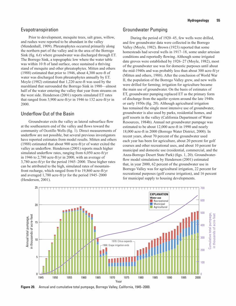
Hydrogeology 55
EvapotranspirationPrior to development, mesquite trees, salt grass, willow,
and rushes were reported to be abundant in the valley (Mendenhall, 1909). Phreatophytes occurred primarily along the northern part of the valley and in the area of the Borrego Sink (fig. 6A) where groundwater was discharged through ET. The Borrego Sink, a topographic low where the water table was within 10 ft of land surface, once sustained a thriving stand of mesquite and other phreatophytes. Mitten and others (1988) estimated that prior to 1946, about 4,300 acre-ft of water was discharged from phreatophytes annually by ET. Moyle (1982) estimated that 1,220 acre-ft was used by the marshland that surrounded the Borrego Sink in 1980—almost half of the water entering the valley that year from streams on the west side. Henderson (2001) reports simulated ET rates that ranged from 3,900 acre-ft/yr in 1946 to 132 acre-ft/yr in 2000.
Underflow Out of the BasinGroundwater exits the valley as lateral subsurface flow
at the southeastern end of the valley and flows toward the community of Ocotillo Wells (fig. 1). Direct measurements of underflow are not possible, but several previous investigators have reported estimates from model results. Mitten and others (1988) estimated that about 900 acre-ft/yr of water exited the valley as underflow. Henderson (2001) reports much higher simulated underflow rates, ranging from 6,050 acre-ft/yr in 1946 to 2,780 acre-ft/yr in 2000, with an average of 3,780 acre-ft/yr for the period 1945–2000. These higher rates can be attributed to the high, simulated rates of mountain-front recharge, which ranged from 0 to 19,860 acre-ft/yr and averaged 1,780 acre-ft/yr for the period 1945–2000 (Henderson, 2001).
Groundwater PumpingDuring the period of 1920–45, few wells were drilled,
and few groundwater data were collected in the Borrego Valley (Moyle, 1982). Brown (1923) reported that some homesteads had several wells in 1917–18, some under artesian conditions and reportedly flowing. Although some irrigated date groves were established by 1926–27 (Moyle, 1982), most of the groundwater use was for domestic purposes until about the mid-1940s and was probably less than about 300 acre-ft/yr (Mitten and others, 1988). After the conclusion of World War II, the population of the Borrego Valley grew, and new wells were drilled for farming; irrigation for agriculture became the main use of groundwater. On the basis of estimates of ET, groundwater pumping replaced ET as the primary form of discharge from the aquifer system around the late 1940s or early 1950s (fig. 20). Although agricultural irrigation has remained the single most intensive use of groundwater, groundwater is also used by parks, residential homes, and golf resorts in the valley (California Department of Water Resources, 1984b). Annual net groundwater pumpage was estimated to be about 12,000 acre-ft in 1990 and nearly 18,000 acre-ft in 2000 (Borrego Water District, 2000). In recent years, about 70 percent of the groundwater used each year has been for agriculture, about 20 percent for golf courses and other recreational uses, and about 10 percent for municipal and domestic use (residential, commercial, and the Anza-Borrego Desert State Park) (figs. 1, 20). Groundwater-flow model simulations by Henderson (2001) estimated that, in year 2000, 62 percent of the groundwater use in Borrego Valley was for agricultural irrigation, 22 percent for recreational purposes (golf course irrigation), and 16 percent for municipal supply to housing developments.
Figure 20. Annual and cumulative total pumpage, Borrego Valley, California, 1945–2000.
sac13-0509_Figure 20 total pumpage
0
100
200
300
400
500
600
700
0
5
10
15
20
25
1945 1950 1955 1960 1965 1970 1975 1980 1985 1990 1995 2000
Cum
ulat
ive
tota
l pum
page
,in
thou
sand
s of
acr
e-fe
et
Annu
al to
tal p
umpa
ge,
in th
ousa
nds
of a
cre-
feet
Year
EXPLANATION
Recreational
Agricultural
Water use
Municipal
1966: Grape irrigation ends1978: Citrus expands
56 Hydrogeology, Hydrologic Effects of Development, and Simulation of Groundwater Flow in the Borrego Valley
Agricultural Water UseHistorically, irrigation for agriculture has been the main
anthropogenic use of groundwater. As mentioned previously, agriculture expanded rapidly after about 1945, and since the late 1940s to early 1950s, the estimated net pumpage, or consumptive use, of groundwater has exceeded estimated natural recharge. Recently, net pumpage was estimated to be approximately four to five times the natural recharge rate (Borrego Valley Water District, 2000; Netto, 2001). The estimates of net pumpage are based on the consumptive use estimated for each land-use type. The land-use types are based on maps, aerial photographs, and other land-use information available for various periods and compiled by Moyle (1982) and Netto (2001). The consumptive use associated with each land-use type is simulated in this study on the basis of the percentage of land cover, reference evapotranspiration, and crop coefficients (KC). The methods used to estimate net pumpage, and the magnitudes of these estimates, are described in more detail in the “Integrated Hydrologic Model” section of this report.
Recreational Water Use
Recreational water use has become the second-largest use of groundwater in the Borrego Valley (Borrego Water District, 2000; Netto, 2001). The primary use of groundwater for recreational activities is irrigation of several golf courses in the valley, including the De Anza Country Club, the Borrego Springs Resort and Country Club operated by the BSPCSD, the Road Runner Golf and Country Club, and the Rams Hill Development (fig. 6K). Netto (2001) describes the history of these courses, which is summarized here. The De Anza Country Club began development in 1953 and reached completion in 1979. During 1963–98, the BSPCSD operated a 9-hole course and expanded it to an 18-hole course in 1998. The Road Runner Country Club golf course began development in 1967 and completed it in about 1979. Construction of the Rams Hill golf course was started in 1982 and was completed in 1983. Historically, the BWD provided groundwater to the Rams Hill Development; details of the pumping for this development, including the golf course, are given in section “Municipal Water Use.” As for agricultural water use, the consumptive use of water by golf courses is simulated in this study on the basis of the percentage of land cover, reference evapotranspiration, and KC; the methodology used to derive the estimates for recreational water use and the magnitudes of these estimates are described in more detail in the “Integrated Hydrologic Model” section of this report.
Municipal Water Use
Compared to crop irrigation and recreational use, municipal water use is a relatively small component of groundwater pumping in the valley; however, municipal water use is well documented. Historical records of municipal pumping have been compiled or estimated for the BWD, which includes the Borrego Springs Water Company, the BSPCSD, and Borrego Air Ranch (BAR; table 5). Total annual municipal pumpage estimates range from
about 110 acre-ft in 1945 (Netto, 2001) to a high of about 4,680 acre-ft in 2007 (J. Rolwing, Borrego Water District, written commun., 2011) (fig. 21). During 1945–2010, the cumulative amount of groundwater pumped was about 153,000 acre-ft.
The BWD is the longest serving water purveyor in the valley. Several water districts have served the valley since 1945, but they have been annexed or acquired by BWD and grouped into Improvement Districts (ID). Pumpage quantities for BWD were reported by well starting in 1983 for the wells in ID4 and in 1984 for wells in ID1 and ID3. ID3 represents the Rancho Borrego Mutual Water Company and the Golden Sand Mutual Water Company, which joined BWD in 1990. BWD purchased Borrego Spring Water Company (BSWC) in 1997, which is represented by ID4. In 2008, BWD began serving the BSPCSD, which is represented by ID5.
The BWD reported annual pumpage by well during 1984–2010 for ID1 wells, 1983–2010 for ID4 wells, and 2005–10 for the ID5 well (table 5). To estimate pumpage for periods when records were not available from BWD or not estimated by Netto (2001), the drillers’ logs were examined to determine when each well was drilled. Annual pumpage at each well was estimated by using the earliest known reported quantity and linearly decreasing that value to zero for the year before each well was drilled. No data were available for the ID4 wells for 1995 from BWD; annual pumpage was assigned the average values for 1994 and 1996. Monthly pumpage data by well were reported by BWD starting in 1987 for ID1 wells, 1997 for ID4 wells, and 1990 for ID3 wells. When monthly pumpage estimates were not available, the annual pumpage data were apportioned on the basis of the average percentage of reported annual pumpage by month for all wells provided by BWD for 1997–2010 (fig. 22).
The BAR supplies water to a small community of homes in the southeastern part of the valley. Although no production records were available, estimates of annual groundwater pumpage were about 10 acre-ft for 1945–2000 (Netto, 2001) and 2001–2010 (J. Rolwing, Borrego Water District, written commun., 2011) (table 5).
Water from BWD’s ID1 wells has been used to irrigate the Rams Hill golf course (fig. 6K) and master-planned community since it was constructed in 1983. During 1983–2010, the amount of water used annually for recreational and municipal purposes in the development ranged between about 630 acre-ft in 2010 and about 1,750 in 2007. During this period, the annual water demand from the Rams Hill development constituted 18–28 percent of the total BWD pumpage (fig. 23). Annual Rams Hill water use from all six ID1 wells for 1983–86 was reported by Netto (2001), and monthly water use for 1987–2010 was reported by Borrego Water District (J. Rolwing, Borrego Water District, written commun., 2011). To distribute the amount of water pumped from ID1 wells that was served to Rams Hill on a monthly basis for the BVHM (see “Integrated Hydrologic Model” section), the average monthly percentage from 1987–2010 was calculated. This average value was used for the monthly values for the years when monthly data were not available.
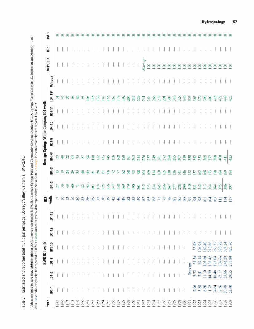
Hydrogeology 57Ta
ble
5.
Estim
ated
and
repo
rted
tota
l mun
icip
al p
umpa
ge, B
orre
go V
alle
y, C
alifo
rnia
, 194
5–20
10.—
Cont
inue
d
[Val
ues r
epor
ted
in a
cre-
feet
. Abb
revi
atio
ns: B
AR
, Bor
rego
Air
Ran
ch, B
SPC
SD, B
orre
go S
prin
gs P
ark
and
Com
mun
ity S
ervi
ces D
istri
ct; B
WD
, Bor
rego
Wat
er D
istri
ct; I
D, I
mpr
ovem
ent D
istri
ct; —
, no
data
. Blu
e in
dica
tes y
early
dat
a re
porte
d by
BW
D; G
reen
indi
cate
s yea
rly d
ata
repo
rted
by N
etto
(200
1); O
rang
e in
dica
tes m
onth
ly d
ata
repo
rted
by B
WD
.
Year
BW
D ID
1 w
ells
ID3
wel
ls
Bor
rego
Spr
ings
Wat
er C
ompa
ny ID
4 w
ells
BSP
CSD
ID5
BA
RID
1-1
ID1-
2ID
1-8
ID1-
10ID
1-12
ID1-
16ID
4-21
ID4-
31ID
4-41
ID4-
5ID
4-10
ID4-
11ID
4-18
1W
ilcox
1945
——
——
——
727
1329
——
—31
——
—10
1946
——
——
——
1038
1940
——
—43
——
—10
1947
——
——
——
1349
2452
——
—56
——
—10
1948
——
——
——
1660
2964
——
—68
——
—10
1949
——
——
——
2071
3575
——
—80
——
—10
1950
——
——
——
2382
4087
——
—93
——
—10
1951
——
——
——
2692
4598
——
—10
5—
——
1019
52—
——
——
—29
103
5111
0—
——
118
——
—10
1953
——
——
——
3311
456
122
——
—13
0—
——
1019
54—
——
——
—36
125
6113
3—
——
142
——
—10
1955
——
——
——
3913
666
145
——
—15
5—
——
1019
56—
——
——
—42
147
7215
6—
——
167
——
—10
1957
——
——
——
4615
877
168
——
—17
9—
——
1019
58—
——
——
—49
169
8218
0—
——
192
——
—10
1959
——
——
——
5217
988
191
——
—20
4—
——
1019
60—
——
——
—55
190
9320
3—
——
217
——
—10
1961
——
——
——
5920
198
214
——
—22
9—
——
1019
62—
——
——
—62
212
104
226
——
—24
1—
Star
t up
—10
1963
——
——
——
6522
310
923
7—
——
254
—10
0—
1019
64—
——
——
—68
234
114
249
——
—26
6—
100
—10
1965
——
——
——
7224
512
026
1—
——
279
—10
0—
1019
66—
——
——
—75
256
125
272
——
—29
1—
100
—10
1967
——
——
——
7826
713
028
4—
——
303
—10
0—
1019
68—
——
——
—81
277
136
295
——
—31
6—
100
—10
1969
——
——
——
8528
814
130
7—
——
328
—10
0—
1019
70—
——
——
—88
299
146
319
——
—34
0—
100
—10
1971
Star
t up
——
9131
015
233
0—
——
353
—10
0—
1019
722.
963.
7234
.56
53.4
8—
—94
321
157
342
——
—36
5—
100
—10
1973
5.88
7.41
69.1
810
6.94
——
9833
216
235
3 —
——
379
—10
0—
1019
748.
8011
.10
103.
8016
0.40
——
101
313
168
365
——
—39
0—
100
—10
1975
11.7
214
.79
138.
4221
3.86
——
104
354
173
377
——
—40
2—
100
—10
1976
14.6
418
.48
173.
0426
7.32
——
107
364
178
388
——
—41
5—
100
—10
1977
17.5
622
.17
207.
6632
0.78
——
111
375
184
400
——
—42
7—
100
—10
1978
20.4
825
.86
242.
2837
4.24
——
114
386
189
411
——
—44
0—
100
—10
1979
23.4
029
.55
276.
9042
7.70
——
117
397
194
423
——
—42
5—
100
—10
Tabl
e 5.
Es
timat
ed a
nd re
porte
d to
tal m
unic
ipal
pum
page
, Bor
rego
Val
ley,
Cal
iforn
ia, 1
945–
2010
.
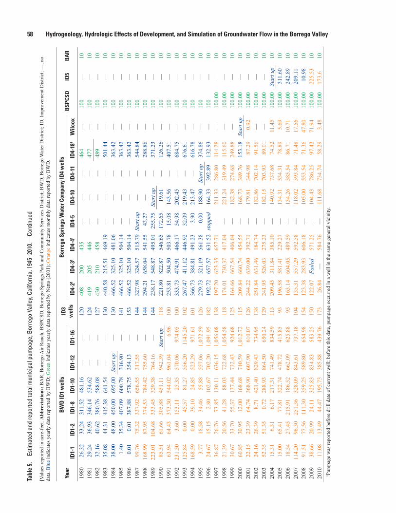
58 Hydrogeology, Hydrologic Effects of Development, and Simulation of Groundwater Flow in the Borrego ValleyTa
ble
5.
Estim
ated
and
repo
rted
tota
l mun
icip
al p
umpa
ge, B
orre
go V
alle
y, C
alifo
rnia
, 194
5–20
10.—
Cont
inue
d
[Val
ues r
epor
ted
in a
cre-
feet
. Abb
revi
atio
ns: B
AR
, Bor
rego
Air
Ran
ch, B
SPC
SD, B
orre
go S
prin
gs P
ark
and
Com
mun
ity S
ervi
ces D
istri
ct; B
WD
, Bor
rego
Wat
er D
istri
ct; I
D, I
mpr
ovem
ent D
istri
ct; —
, no
data
. Blu
e in
dica
tes y
early
dat
a re
porte
d by
BW
D; G
reen
indi
cate
s yea
rly d
ata
repo
rted
by N
etto
(200
1); O
rang
e in
dica
tes m
onth
ly d
ata
repo
rted
by B
WD
.
Year
BW
D ID
1 w
ells
ID3
wel
ls
Bor
rego
Spr
ings
Wat
er C
ompa
ny ID
4 w
ells
BSP
CSD
ID5
BA
RID
1-1
ID1-
2ID
1-8
ID1-
10ID
1-12
ID1-
16ID
4-21
ID4-
31ID
4-41
ID4-
5ID
4-10
ID4-
11ID
4-18
1W
ilcox
1980
26.3
233
.24
311.
5248
1.16
——
120
408
200
435
——
—46
4—
100
—10
1981
29.2
436
.93
346.
1453
4.62
——
124
419
205
446
——
—47
7—
100
—10
1982
32.1
640
.62
380.
7658
8.08
——
127
430
210
458
——
—48
9—
100
—10
1983
35.0
844
.31
415.
3864
1.54
——
130
440.
5821
5.51
469.
19—
——
501.
44—
100
—10
1984
38.0
048
.00
450.
0069
5.00
Star
t up
—13
046
6.52
325.
1048
1.06
——
—36
3.42
—10
0—
1019
851.
4035
.34
407.
0960
0.78
316.
90—
141
466.
5232
5.10
504.
14—
——
363.
42—
100
—10
1986
0.01
0.01
387.
8857
8.75
354.
13—
153
466.
5232
5.10
504.
14—
——
363.
42—
100
—10
1987
99.7
675
.32
337.
9265
6.55
317.
55—
144
327.
9832
4.57
515.
79St
art u
p—
—54
4.84
—10
0—
1019
8816
8.99
87.9
537
4.53
784.
4275
5.60
—14
429
4.21
658.
0454
1.55
43.2
7—
—28
8.86
—10
0—
1019
8922
3.01
104.
6833
3.45
329.
3876
4.16
—14
423
8.17
548.
8749
5.01
255.
75St
art u
p—
371.
23—
100
—10
1990
85.5
161
.66
305.
8845
1.11
942.
39St
art u
p11
822
1.80
822.
8754
6.65
172.
6519
.61
—12
6.26
—10
0—
1019
9163
.94
64.4
337
3.30
544.
0296
1.04
6.96
100
253.
8150
4.50
503.
7815
.08
143.
56—
407.
51—
100
—10
1992
231.
503.
6015
3.11
25.3
557
0.06
974.
0510
033
3.73
474.
9146
6.17
54.9
820
2.45
—68
4.75
—10
0—
1019
9312
5.84
0.00
45.5
781
.27
556.
2011
45.2
010
226
7.47
411.
1244
6.92
32.0
921
9.43
—67
6.61
—10
0—
1019
9416
8.59
0.00
39.1
024
.85
523.
2997
1.61
101
366.
7338
4.81
491.
233.
9021
3.47
—61
6.78
—10
0—
1019
953.
7718
.58
34.4
655
.88
557.
061,
072.
5912
627
9.73
521.
1956
1.38
0.00
188.
90St
art u
p37
4.86
—10
0—
1019
9624
.67
15.1
52.
8010
2.67
702.
201,
091.
9518
219
2.72
657.
5763
1.52
stop
ped
164.
3339
2.89
132.
93—
100
—10
1997
36.8
726
.76
73.8
513
0.11
636.
151,
056.
0813
819
7.20
623.
3565
7.71
—21
1.33
286.
8011
4.28
—10
0.00
—10
1998
21.3
920
.56
41.2
888
.03
722.
681,
054.
5811
817
4.01
730.
3741
7.04
—22
1.24
319.
4911
5.60
—10
0.00
—10
1999
30.6
733
.70
55.3
713
7.44
732.
4392
4.68
125
164.
6666
7.54
406.
04—
182.
3827
4.68
249.
88—
100.
00—
1020
0060
.85
30.9
512
.00
168.
6871
0.59
1,01
2.72
115
209.
8466
0.74
454.
55—
168.
7338
9.76
153.
18St
art u
p10
0.00
—10
2001
22.1
523
.39
64.7
436
8.90
607.
9061
0.07
126
244.
2263
9.00
392.
71—
179.
8134
4.98
87.2
90.
9210
0.00
—10
2002
24.1
626
.39
8.71
421.
4082
9.43
734.
9513
825
1.84
631.
4618
4.74
—18
2.86
702.
1491
.56
—10
0.00
—10
2003
52.3
551
.35
0.72
288.
9386
4.50
650.
2412
924
1.95
526.
0327
5.23
—18
2.15
703.
9389
.01
—10
0.00
—10
2004
15.3
16.
316.
1721
7.31
741.
4983
4.59
113
209.
4531
1.84
385.
10—
140.
9273
7.68
74.5
211
.45
100.
00St
art u
p10
2005
15.0
065
.41
77.8
132
2.74
478.
7241
5.85
9319
6.58
581.
4122
9.27
—13
4.31
534.
3178
.89
5.69
100.
0031
1.60
1020
0618
.54
27.4
521
5.91
186.
5266
2.09
625.
8895
163.
1460
4.05
489.
59—
134.
2638
5.54
86.7
110
.71
100.
0024
2.89
1020
0711
4.20
96.3
025
1.36
328.
0984
3.61
737.
1810
413
5.31
557.
2959
2.58
—11
8.02
393.
8471
.48
17.5
610
0.00
209.
1110
2008
91.5
177
.56
111.
3035
9.25
589.
8065
4.98
154
123.
3828
3.93
606.
18—
105.
0055
3.54
71.3
647
.80
100.
0010
.98
1020
0938
.66
20.9
924
.11
325.
8383
4.83
583.
2515
012
2.07
Faile
d57
1.25
—10
4.43
786.
2597
.42
71.9
410
0.00
225.
5310
2010
11.0
813
.49
44.4
719
5.73
385.
8843
9.76
173
26.8
4—
584.
76—
111.
6873
4.74
58.2
93.
4810
0.00
173.
610
1 Pum
page
was
repo
rted
befo
re d
rill d
ate
of c
urre
nt w
ell;
befo
re th
is d
ate,
pum
page
occ
urre
d in
a w
ell i
n th
e sa
me
gene
ral v
icin
ity.
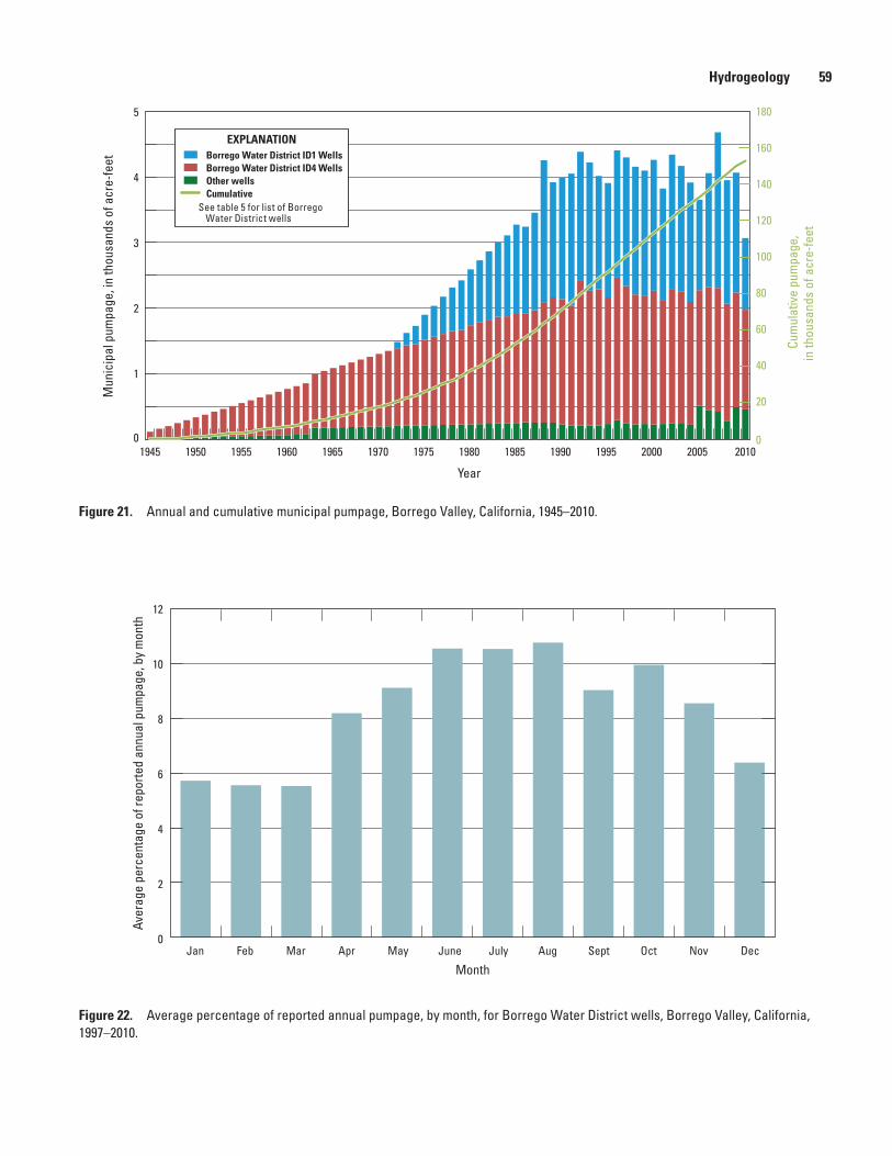
Hydrogeology 59
Figure 21. Annual and cumulative municipal pumpage, Borrego Valley, California, 1945–2010.
Figure 22. Average percentage of reported annual pumpage, by month, for Borrego Water District wells, Borrego Valley, California, 1997–2010.
sac13-0509_Figure 21 BW-Q
0
20
40
60
80
100
120
140
160
180
01945 1950 1955 1960 1965 1970 1975 1980
Year
1985 1990 1995 2000 2005 2010
1
2
3
4
5
Cum
ulat
ive
pum
page
,in
thou
sand
s of
acr
e-fe
et
Mun
icip
al p
umpa
ge, i
n th
ousa
nds
of a
cre-
feet
Borrego Water District ID1 WellsBorrego Water District ID4 WellsOther wellsCumulative
See table 5 for list of Borrego Water District wells
EXPLANATION
sac13-0509_Figure 22 BW-Q percent
0
2
4
6
8
10
12
Jan Feb Mar Apr May June July Aug Sept Oct Nov Dec
Aver
age
perc
enta
ge o
f rep
orte
d an
nual
pum
page
, by
mon
th
Month
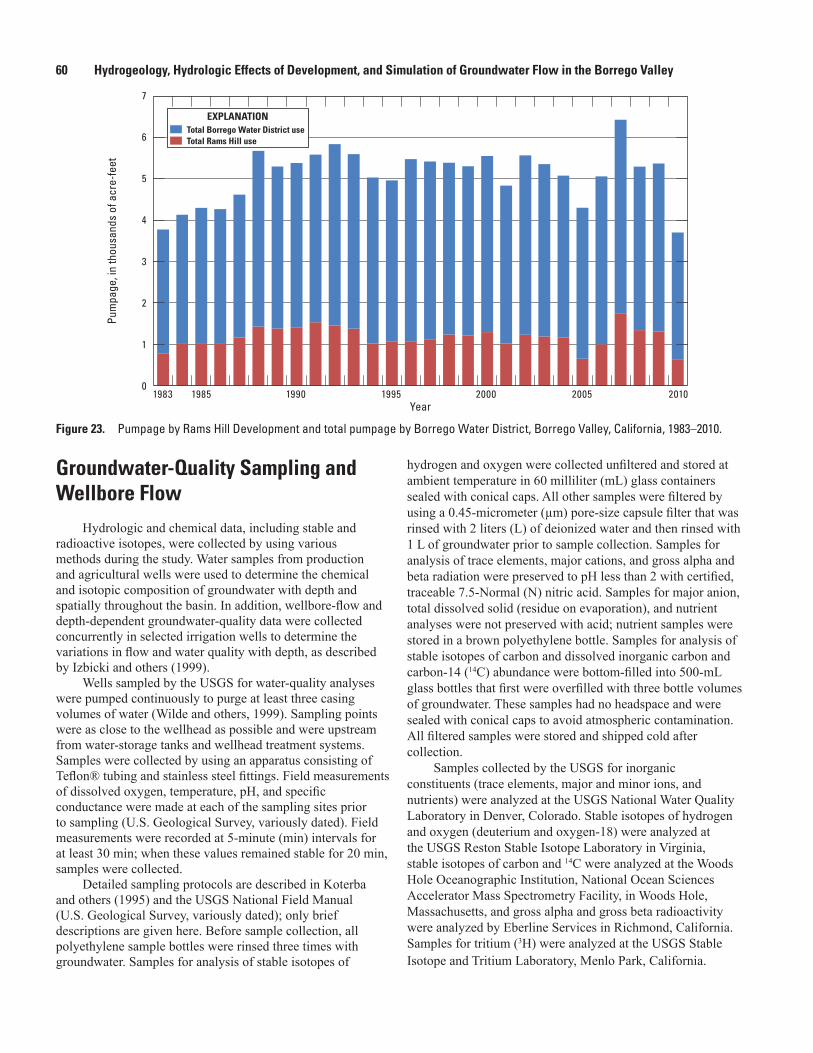
60 Hydrogeology, Hydrologic Effects of Development, and Simulation of Groundwater Flow in the Borrego Valley
Groundwater-Quality Sampling and Wellbore Flow
Hydrologic and chemical data, including stable and radioactive isotopes, were collected by using various methods during the study. Water samples from production and agricultural wells were used to determine the chemical and isotopic composition of groundwater with depth and spatially throughout the basin. In addition, wellbore-flow and depth-dependent groundwater-quality data were collected concurrently in selected irrigation wells to determine the variations in flow and water quality with depth, as described by Izbicki and others (1999).
Wells sampled by the USGS for water-quality analyses were pumped continuously to purge at least three casing volumes of water (Wilde and others, 1999). Sampling points were as close to the wellhead as possible and were upstream from water-storage tanks and wellhead treatment systems. Samples were collected by using an apparatus consisting of Teflon® tubing and stainless steel fittings. Field measurements of dissolved oxygen, temperature, pH, and specific conductance were made at each of the sampling sites prior to sampling (U.S. Geological Survey, variously dated). Field measurements were recorded at 5-minute (min) intervals for at least 30 min; when these values remained stable for 20 min, samples were collected.
Detailed sampling protocols are described in Koterba and others (1995) and the USGS National Field Manual (U.S. Geological Survey, variously dated); only brief descriptions are given here. Before sample collection, all polyethylene sample bottles were rinsed three times with groundwater. Samples for analysis of stable isotopes of
hydrogen and oxygen were collected unfiltered and stored at ambient temperature in 60 milliliter (mL) glass containers sealed with conical caps. All other samples were filtered by using a 0.45-micrometer (µm) pore-size capsule filter that was rinsed with 2 liters (L) of deionized water and then rinsed with 1 L of groundwater prior to sample collection. Samples for analysis of trace elements, major cations, and gross alpha and beta radiation were preserved to pH less than 2 with certified, traceable 7.5-Normal (N) nitric acid. Samples for major anion, total dissolved solid (residue on evaporation), and nutrient analyses were not preserved with acid; nutrient samples were stored in a brown polyethylene bottle. Samples for analysis of stable isotopes of carbon and dissolved inorganic carbon and carbon-14 (14C) abundance were bottom-filled into 500-mL glass bottles that first were overfilled with three bottle volumes of groundwater. These samples had no headspace and were sealed with conical caps to avoid atmospheric contamination. All filtered samples were stored and shipped cold after collection.
Samples collected by the USGS for inorganic constituents (trace elements, major and minor ions, and nutrients) were analyzed at the USGS National Water Quality Laboratory in Denver, Colorado. Stable isotopes of hydrogen and oxygen (deuterium and oxygen-18) were analyzed at the USGS Reston Stable Isotope Laboratory in Virginia, stable isotopes of carbon and 14C were analyzed at the Woods Hole Oceanographic Institution, National Ocean Sciences Accelerator Mass Spectrometry Facility, in Woods Hole, Massachusetts, and gross alpha and gross beta radioactivity were analyzed by Eberline Services in Richmond, California. Samples for tritium (3H) were analyzed at the USGS Stable Isotope and Tritium Laboratory, Menlo Park, California.
Figure 23. Pumpage by Rams Hill Development and total pumpage by Borrego Water District, Borrego Valley, California, 1983–2010.
sac13-0509_Figure 23 BWD_RamsHill
0
1
2
3
4
5
6
7
Pum
page
, in
thou
sand
s of
acr
e-fe
et
1983 1985 1990 1995Year
2000 2005 2010
Total Borrego Water District useTotal Rams Hill use
EXPLANATION
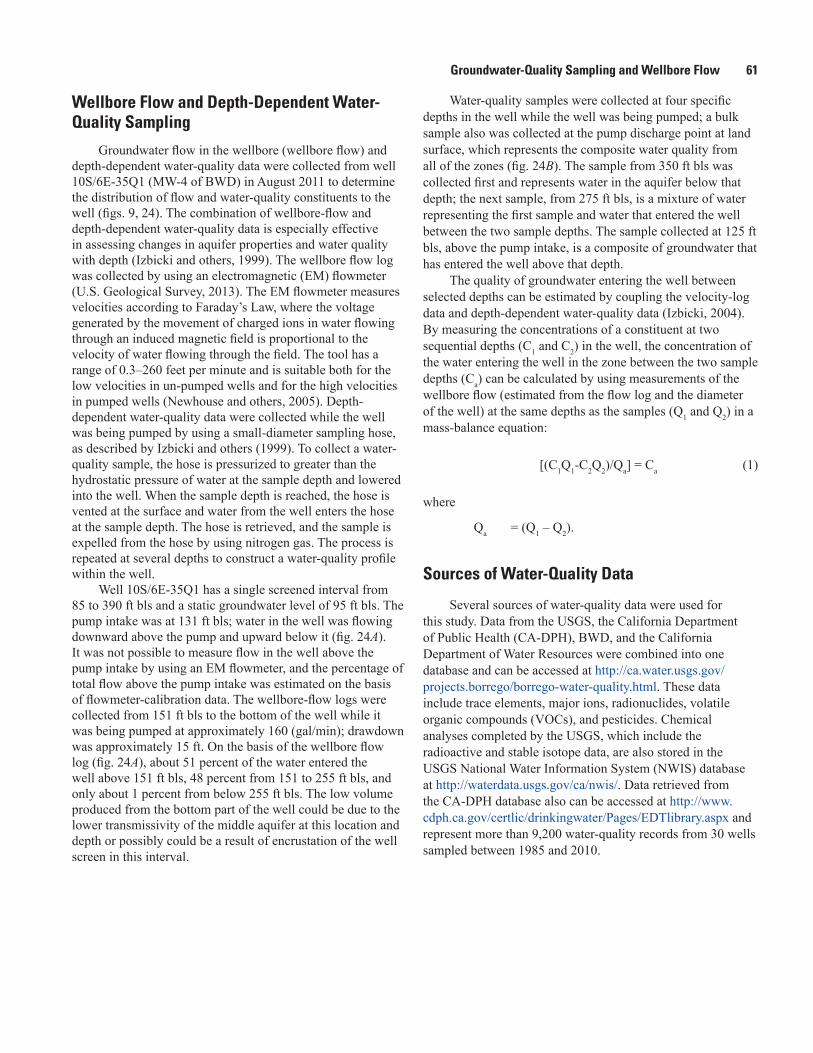
Groundwater-Quality Sampling and Wellbore Flow 61
Wellbore Flow and Depth-Dependent Water-Quality Sampling
Groundwater flow in the wellbore (wellbore flow) and depth-dependent water-quality data were collected from well 10S/6E-35Q1 (MW-4 of BWD) in August 2011 to determine the distribution of flow and water-quality constituents to the well (figs. 9, 24). The combination of wellbore-flow and depth-dependent water-quality data is especially effective in assessing changes in aquifer properties and water quality with depth (Izbicki and others, 1999). The wellbore flow log was collected by using an electromagnetic (EM) flowmeter (U.S. Geological Survey, 2013). The EM flowmeter measures velocities according to Faraday’s Law, where the voltage generated by the movement of charged ions in water flowing through an induced magnetic field is proportional to the velocity of water flowing through the field. The tool has a range of 0.3–260 feet per minute and is suitable both for the low velocities in un-pumped wells and for the high velocities in pumped wells (Newhouse and others, 2005). Depth-dependent water-quality data were collected while the well was being pumped by using a small-diameter sampling hose, as described by Izbicki and others (1999). To collect a water-quality sample, the hose is pressurized to greater than the hydrostatic pressure of water at the sample depth and lowered into the well. When the sample depth is reached, the hose is vented at the surface and water from the well enters the hose at the sample depth. The hose is retrieved, and the sample is expelled from the hose by using nitrogen gas. The process is repeated at several depths to construct a water-quality profile within the well.
Well 10S/6E-35Q1 has a single screened interval from 85 to 390 ft bls and a static groundwater level of 95 ft bls. The pump intake was at 131 ft bls; water in the well was flowing downward above the pump and upward below it (fig. 24A). It was not possible to measure flow in the well above the pump intake by using an EM flowmeter, and the percentage of total flow above the pump intake was estimated on the basis of flowmeter-calibration data. The wellbore-flow logs were collected from 151 ft bls to the bottom of the well while it was being pumped at approximately 160 (gal/min); drawdown was approximately 15 ft. On the basis of the wellbore flow log (fig. 24A), about 51 percent of the water entered the well above 151 ft bls, 48 percent from 151 to 255 ft bls, and only about 1 percent from below 255 ft bls. The low volume produced from the bottom part of the well could be due to the lower transmissivity of the middle aquifer at this location and depth or possibly could be a result of encrustation of the well screen in this interval.
Water-quality samples were collected at four specific depths in the well while the well was being pumped; a bulk sample also was collected at the pump discharge point at land surface, which represents the composite water quality from all of the zones (fig. 24B). The sample from 350 ft bls was collected first and represents water in the aquifer below that depth; the next sample, from 275 ft bls, is a mixture of water representing the first sample and water that entered the well between the two sample depths. The sample collected at 125 ft bls, above the pump intake, is a composite of groundwater that has entered the well above that depth.
The quality of groundwater entering the well between selected depths can be estimated by coupling the velocity-log data and depth-dependent water-quality data (Izbicki, 2004). By measuring the concentrations of a constituent at two sequential depths (C1 and C2) in the well, the concentration of the water entering the well in the zone between the two sample depths (Ca) can be calculated by using measurements of the wellbore flow (estimated from the flow log and the diameter of the well) at the same depths as the samples (Q1 and Q2) in a mass-balance equation:
[(C1Q1-C2Q2)/Qa] = Ca (1)
where
Qa = (Q1 – Q2).
Sources of Water-Quality Data
Several sources of water-quality data were used for this study. Data from the USGS, the California Department of Public Health (CA-DPH), BWD, and the California Department of Water Resources were combined into one database and can be accessed at http://ca.water.usgs.gov/projects.borrego/borrego-water-quality.html. These data include trace elements, major ions, radionuclides, volatile organic compounds (VOCs), and pesticides. Chemical analyses completed by the USGS, which include the radioactive and stable isotope data, are also stored in the USGS National Water Information System (NWIS) database at http://waterdata.usgs.gov/ca/nwis/. Data retrieved from the CA-DPH database also can be accessed at http://www.cdph.ca.gov/certlic/drinkingwater/Pages/EDTlibrary.aspx and represent more than 9,200 water-quality records from 30 wells sampled between 1985 and 2010.
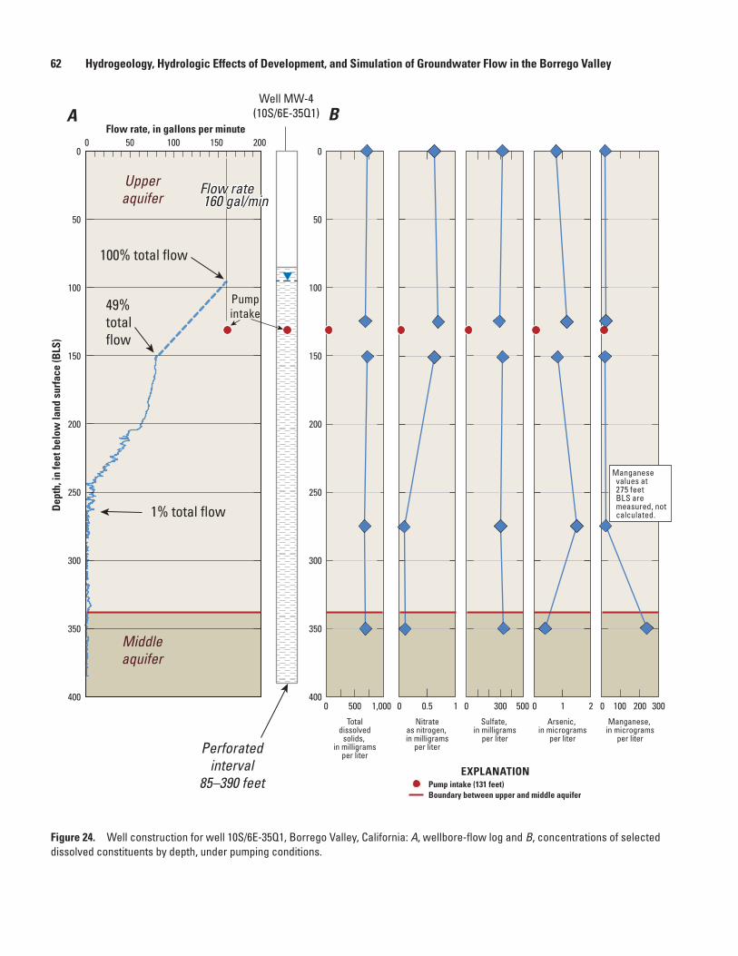
62 Hydrogeology, Hydrologic Effects of Development, and Simulation of Groundwater Flow in the Borrego Valley
Figure 24. Well construction for well 10S/6E-35Q1, Borrego Valley, California: A, wellbore-flow log and B, concentrations of selected dissolved constituents by depth, under pumping conditions.sac13-0509_Figure 24ab MW-4 QW
0 500 1,000
Totaldissolved
solids, in milligrams
per liter
Nitrateas nitrogen, in milligrams
per liter
0 10.5 0 21 0 100 200 300
Sulfate, in milligrams
per liter
Arsenic, in micrograms
per liter
Manganese, in micrograms
per liter
0 300 500
Dep
th, i
n fe
et b
elow
land
sur
face
(BLS
)
0 50 100 150 200Flow rate, in gallons per minute
1% total flow
100% total flow
49%totalflow
Well MW-4(10S/6E-35Q1)A B
0
50
100
150
200
250
300
350
400
0
50
100
150
200
250
300
350
400
Upperaquifer
Middleaquifer
Perforatedinterval
85–390 feet
Flow rate160 gal/min
Pumpintake
Manganese values at 275 feet BLS are measured, not calculated.
EXPLANATION
Boundary between upper and middle aquiferPump intake (131 feet)
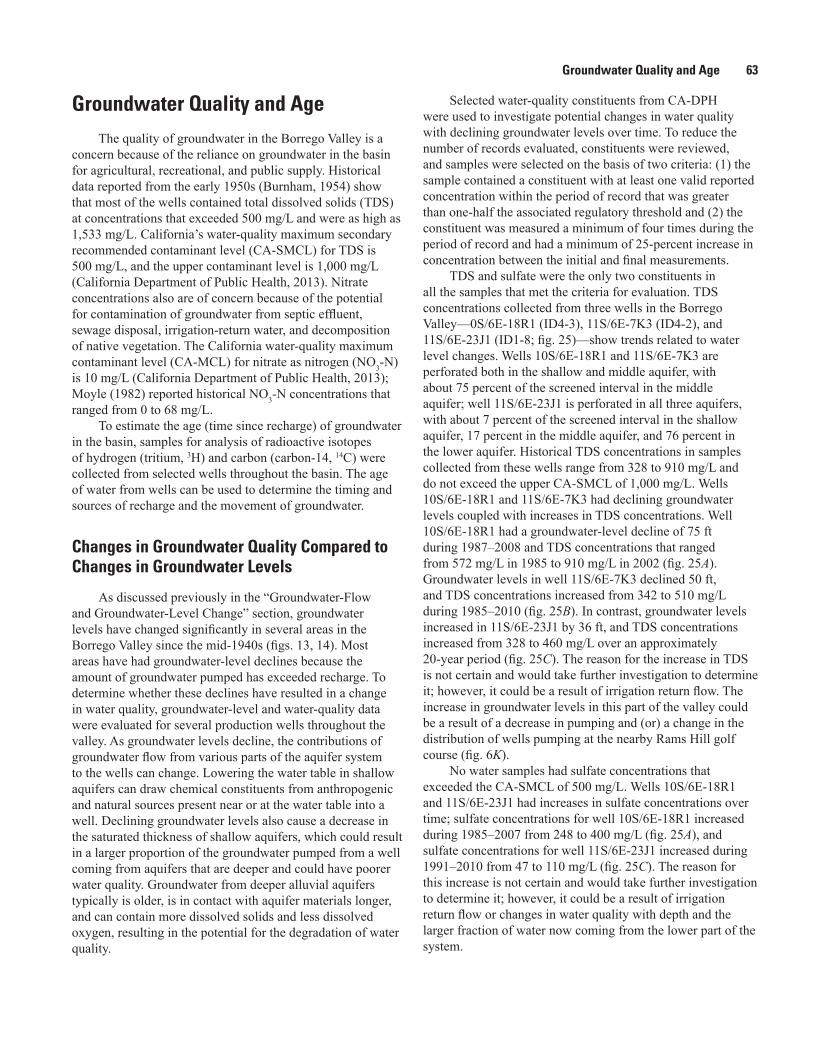
Groundwater Quality and Age 63
Groundwater Quality and AgeThe quality of groundwater in the Borrego Valley is a
concern because of the reliance on groundwater in the basin for agricultural, recreational, and public supply. Historical data reported from the early 1950s (Burnham, 1954) show that most of the wells contained total dissolved solids (TDS) at concentrations that exceeded 500 mg/L and were as high as 1,533 mg/L. California’s water-quality maximum secondary recommended contaminant level (CA-SMCL) for TDS is 500 mg/L, and the upper contaminant level is 1,000 mg/L (California Department of Public Health, 2013). Nitrate concentrations also are of concern because of the potential for contamination of groundwater from septic effluent, sewage disposal, irrigation-return water, and decomposition of native vegetation. The California water-quality maximum contaminant level (CA-MCL) for nitrate as nitrogen (NO3-N) is 10 mg/L (California Department of Public Health, 2013); Moyle (1982) reported historical NO3-N concentrations that ranged from 0 to 68 mg/L.
To estimate the age (time since recharge) of groundwater in the basin, samples for analysis of radioactive isotopes of hydrogen (tritium, 3H) and carbon (carbon-14, 14C) were collected from selected wells throughout the basin. The age of water from wells can be used to determine the timing and sources of recharge and the movement of groundwater.
Changes in Groundwater Quality Compared to Changes in Groundwater Levels
As discussed previously in the “Groundwater-Flow and Groundwater-Level Change” section, groundwater levels have changed significantly in several areas in the Borrego Valley since the mid-1940s (figs. 13, 14). Most areas have had groundwater-level declines because the amount of groundwater pumped has exceeded recharge. To determine whether these declines have resulted in a change in water quality, groundwater-level and water-quality data were evaluated for several production wells throughout the valley. As groundwater levels decline, the contributions of groundwater flow from various parts of the aquifer system to the wells can change. Lowering the water table in shallow aquifers can draw chemical constituents from anthropogenic and natural sources present near or at the water table into a well. Declining groundwater levels also cause a decrease in the saturated thickness of shallow aquifers, which could result in a larger proportion of the groundwater pumped from a well coming from aquifers that are deeper and could have poorer water quality. Groundwater from deeper alluvial aquifers typically is older, is in contact with aquifer materials longer, and can contain more dissolved solids and less dissolved oxygen, resulting in the potential for the degradation of water quality.
Selected water-quality constituents from CA-DPH were used to investigate potential changes in water quality with declining groundwater levels over time. To reduce the number of records evaluated, constituents were reviewed, and samples were selected on the basis of two criteria: (1) the sample contained a constituent with at least one valid reported concentration within the period of record that was greater than one-half the associated regulatory threshold and (2) the constituent was measured a minimum of four times during the period of record and had a minimum of 25-percent increase in concentration between the initial and final measurements.
TDS and sulfate were the only two constituents in all the samples that met the criteria for evaluation. TDS concentrations collected from three wells in the Borrego Valley—0S/6E-18R1 (ID4-3), 11S/6E-7K3 (ID4-2), and 11S/6E-23J1 (ID1-8; fig. 25)—show trends related to water level changes. Wells 10S/6E-18R1 and 11S/6E-7K3 are perforated both in the shallow and middle aquifer, with about 75 percent of the screened interval in the middle aquifer; well 11S/6E-23J1 is perforated in all three aquifers, with about 7 percent of the screened interval in the shallow aquifer, 17 percent in the middle aquifer, and 76 percent in the lower aquifer. Historical TDS concentrations in samples collected from these wells range from 328 to 910 mg/L and do not exceed the upper CA-SMCL of 1,000 mg/L. Wells 10S/6E-18R1 and 11S/6E-7K3 had declining groundwater levels coupled with increases in TDS concentrations. Well 10S/6E-18R1 had a groundwater-level decline of 75 ft during 1987–2008 and TDS concentrations that ranged from 572 mg/L in 1985 to 910 mg/L in 2002 (fig. 25A). Groundwater levels in well 11S/6E-7K3 declined 50 ft, and TDS concentrations increased from 342 to 510 mg/L during 1985–2010 (fig. 25B). In contrast, groundwater levels increased in 11S/6E-23J1 by 36 ft, and TDS concentrations increased from 328 to 460 mg/L over an approximately 20-year period (fig. 25C). The reason for the increase in TDS is not certain and would take further investigation to determine it; however, it could be a result of irrigation return flow. The increase in groundwater levels in this part of the valley could be a result of a decrease in pumping and (or) a change in the distribution of wells pumping at the nearby Rams Hill golf course (fig. 6K).
No water samples had sulfate concentrations that exceeded the CA-SMCL of 500 mg/L. Wells 10S/6E-18R1 and 11S/6E-23J1 had increases in sulfate concentrations over time; sulfate concentrations for well 10S/6E-18R1 increased during 1985–2007 from 248 to 400 mg/L (fig. 25A), and sulfate concentrations for well 11S/6E-23J1 increased during 1991–2010 from 47 to 110 mg/L (fig. 25C). The reason for this increase is not certain and would take further investigation to determine it; however, it could be a result of irrigation return flow or changes in water quality with depth and the larger fraction of water now coming from the lower part of the system.
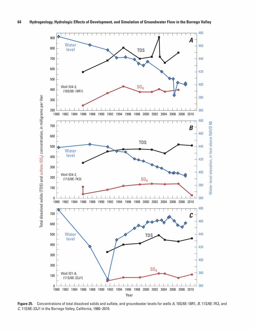
64 Hydrogeology, Hydrologic Effects of Development, and Simulation of Groundwater Flow in the Borrego Valley
Figure 25. Concentrations of total dissolved solids and sulfate, and groundwater levels for wells A, 10S/6E-18R1, B, 11S/6E-7K3, and C, 11S/6E-23J1 in the Borrego Valley, California, 1980–2010.
Year
Well ID4-3, (10S/6E-18R1)
Well ID4-2, (11S/6E-7K3)
Well ID1-8, (11S/6E-23J1)
Tota
l dis
solv
ed s
olid
s (T
DS) a
nd s
ulfa
te (S
O 4) c
once
ntra
tion,
in m
illig
ram
s pe
r lite
r
360
380
400
420
440
460
480
360
380
400
420
440
460
480
360
380
400
420
440
460
480
200
300
400
500
600
700
800
900
0
100
200
300
400
500
600
700
0
100
200
300
400
500
600
700W
ater
-leve
l ele
vatio
n, in
feet
abo
ve N
AVD
88
SO4
SO4
SO4
TDS
Waterlevel
Waterlevel
Waterlevel
TDS
TDS
1980 1982 1984 1986 1988 1990 1992 1994 1996 1998 2000 2002 2004 2006 2006 2010
1980 1982 1984 1986 1988 1990 1992 1994 1996 1998 2000 2002 2004 2006 2006 2010
1980 1982 1984 1986 1988 1990 1992 1994 1996 1998 2000 2002 2004 2006 2006 2010
sac13-0509_Figure 25 QW-WL
A
B
C
Groundwater Quality and Age 65
Distribution and Variation of Groundwater Quality
Water-quality data gathered from individual wells for this study were evaluated to determine whether any chemical constituents sampled exceeded either the California maximum contaminant level (CA-MCL) or California secondary maximum contaminant level (CA-SMCL). These data can be reviewed in the database created for this study (http://ca.water.usgs.gov/projects.borrego/borrego-water-quality.html). With the exception of three fluoride concentrations from three wells that ranged from 2.69 to 4.87 mg/L (the CA-MCL is 2 mg/L), only nitrate and TDS concentrations frequently exceeded the CA-MCL and CA-SMCL, respectively. Moyle (1982) reports that historical data from the agricultural area in the northern part of the basin showed that some shallow wells contained groundwater that exceeded the CA-MCL of 10 mg/L for NO3-N and the CA-SMCL of 1,500 mg/L for TDS. In an effort to improve the quality of the water from their wells, some landowners either abandoned or destroyed wells perforated in the upper aquifer and installed deeper wells perforated only in the middle and lower aquifers. As a result, recent water-quality data for the shallow aquifer are sparse, and the evaluation of water quality in the shallow aquifer for this study was based predominantly on historical data reported by Moyle (1982) and Burnham (1954) and recorded in well files in the USGS project office in San Diego, California.
Distribution of Nitrates and Total Dissolved Solids
Water-quality samples from wells distributed throughout the valley show that NO3-N concentrations ranged from less than 1 mg/L to almost 67 mg/L. NO3-N concentrations were highest in the shallow aquifer and exceeded the CA-MCL of 10 mg/L in some samples from the shallow and middle aquifers in the northwestern part of the basin (fig. 26). NO3-N concentrations in samples from the lower aquifer did not exceed 6.7 mg/L.
Water-quality data show that TDS concentrations ranged from less than 500 mg/L to as high as 2,330 mg/L. Similar to the nitrate concentrations, the maximum TDS concentrations were in samples from the shallow aquifer and generally were highest in the northwestern part of the basin (fig. 27). TDS concentrations in samples from the middle aquifer were as high as 1,350 mg/L. With the exception of one sample, TDS concentrations in the lower aquifer did not exceed the CA-SMCL of 1,000 mg/L, and most samples had TDS concentrations lower than those in samples from the upper and middle aquifers.
Three wells in the northern part of the basin were sampled in 2011 in an effort to obtain recent water-quality data from adjacent wells to relate nitrate and TDS concentrations to depth. As was documented by Moyle (1982), most, if not all, shallow wells in this part of the basin have been either destroyed or abandoned because of poor water quality. Consequently, it was possible to sample wells perforated only in the middle and lower aquifers. Wells 10S/6E-15D3 and 10S/6E-15D4 are perforated exclusively in the middle aquifer, and well 10S/6E-21A2 has 90 percent of its perforations in the lower aquifer. The top of the perforations of well 10S/6E-15D4 are 180 ft above the top of the perforations in well 10S/6E-15D3. Therefore, of these three wells, 10S/6E-15D4 is considered the shallowest site, 10S/6E-15D3 is considered the mid-depth site, and 10S/6E-21A2 is considered the deepest site.
Samples collected from 10S/6E-15D4 (shallowest site) had the poorest groundwater quality of the three wells (http://ca.water.usgs.gov/projects.borrego/borrego-water-quality.html). The NO3-N concentration was 37.3 mg/L, which was at least 40 times more than those for the two deeper wells. Nitrate concentrations in samples from wells 10S/6E-15D3 (mid-depth site) and 10S/6E-21A2 (deepest site) were 0.92 mg/L and 0.02 mg/L, respectively. The two deeper wells did not have any constituents’ concentrations greater than the regulatory thresholds. However, samples collected from well 10S/6E-15D3 had molybdenum and fluoride concentrations of 38.9 µg/L and 1.69 mg/L, respectively, which were near the U.S. Environmental Protection Agency lifetime health advisory level of 40 micrograms per liter (µg/L) for molybdenum and the CA-MCL of 2 mg/L for fluoride. Samples from well 10S/6E-21A2 had molybdenum and fluoride concentrations of 33.1 µg/L and 0.75 mg/L, respectively. The TDS concentration in well 10S/6E-15D4 was 1,350 mg/L, which was twice the concentration in well 10S/6E-15D3 and almost three times the concentration in well 10S/6E-21A2. Possible causes of increasing TDS in wells include irrigation with saline water, the downward movement of salts that have accumulated in the unsaturated zone, and the dissolution of evaporative minerals (Suarez, 1989). In arid areas, salts build up in the unsaturated zone over thousands of years and can be mobilized by irrigation water, subsequently degrading groundwater quality (Scanlon and others, 2007).
Variations in Water Quality with DepthGroundwater flow and depth-dependent water-quality
data were collected from well 10S/6E-35Q1 to determine whether there were variations in the distribution of flow or chemical constituents with depth (fig. 24). The sample of water collected at the surface, or the bulk sample, is a composite of the water quality from all producing zones in the
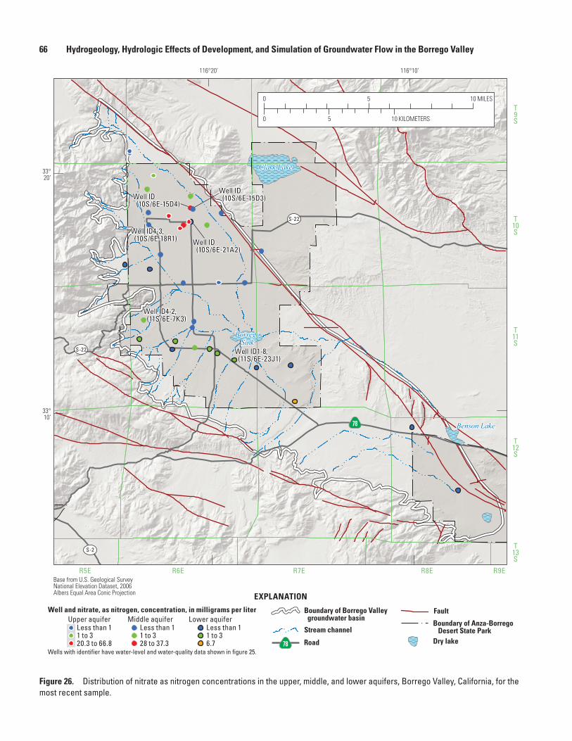
66 Hydrogeology, Hydrologic Effects of Development, and Simulation of Groundwater Flow in the Borrego Valley
Figure 26. Distribution of nitrate as nitrogen concentrations in the upper, middle, and lower aquifers, Borrego Valley, California, for the most recent sample.
Clark Lake
BorregoSink
Benson Lake
T9S
T10S
T11S
T12S
T13S
R5E R6E R7E R8E R9EBase from U.S. Geological Survey National Elevation Dataset, 2006Albers Equal Area Conic Projection
S-22
S-22
S-2
78
116°10’116°20’
33°20’
33°10’
0
0 5 10
5 10 MILES
KILOMETERS
sac13-0509_Figure 26 NO3 by layer-upper, middle & lower
EXPLANATION
Well and nitrate, as nitrogen, concentration, in milligrams per liter
Less than 11 to 320.3 to 66.8
Upper aquifer Middle aquiferLess than 11 to 328 to 37.3
Lower aquiferLess than 11 to 36.7
Stream channel
Boundary of Borrego Valley groundwater basin
Wells with identifier have water-level and water-quality data shown in figure 25.Road78
Well ID4-3, (10S/6E-18R1)
Well ID (10S/6E-15D4)
Well ID (10S/6E-15D3)
Well ID (10S/6E-21A2)
Well ID4-2, (11S/6E-7K3)
Well ID1-8, (11S/6E-23J1)
Boundary of Anza-Borrego Desert State Park
Fault
Dry lake
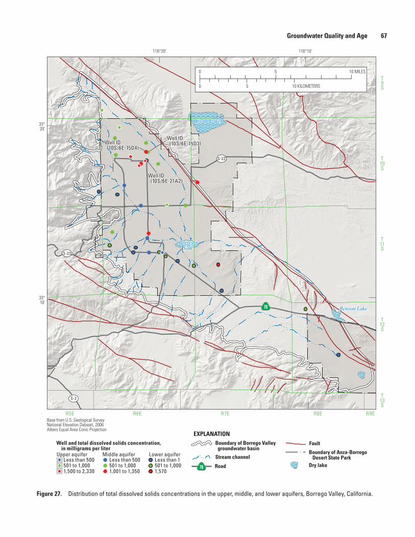
Groundwater Quality and Age 67
Figure 27. Distribution of total dissolved solids concentrations in the upper, middle, and lower aquifers, Borrego Valley, California.
Clark Lake
BorregoSink
Benson Lake
T9S
T10S
T11S
T12S
T13S
R5E R6E R7E R8E R9EBase from U.S. Geological Survey National Elevation Dataset, 2006Albers Equal Area Conic Projection
S-22
S-22
S-2
78
116°10’116°20’
33°20’
33°10’
0
0 5 10
5 10 MILES
KILOMETERS
sac13-0509_Figure 27 TDS by layer
Stream channel
Boundary of Borrego Valley groundwater basin
Well and total dissolved solids concentration, in milligrams per liter
Less than 500501 to 1,0001,500 to 2,330
Upper aquifer Lower aquiferLess than 1501 to 1,0001,570
Middle aquiferLess than 500501 to 1,0001,001 to 1,350
Road78
EXPLANATION
Boundary of Anza-Borrego Desert State Park
Fault
Dry lake
Well ID (10S/6E-15D4)
Well ID (10S/6E-15D3)
Well ID (10S/6E-21A2)
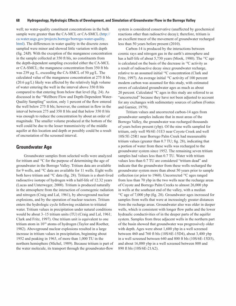
68 Hydrogeology, Hydrologic Effects of Development, and Simulation of Groundwater Flow in the Borrego Valley
well; no water-quality constituent concentrations in the bulk sample were greater than the CA-MCL or CA-SMCL (http://ca.water.usgs.gov/projects.borrego/borrego-water-quality.html). The differences in water quality in the discrete zones sampled were minor and showed little variation with depth (fig. 24B). With the exception of the manganese concentration in the sample collected at 350 ft bls, no constituents from the depth-dependent sampling exceeded either the CA-MCL or CA-SMCL; the manganese concentration from 350 ft bls was 239 µg /L, exceeding the CA-SMCL of 50 µg/L. The calculated value of the manganese concentration at 275 ft bls (20.6 µg/L) likely was affected by the relatively high volume of water entering the well in the interval above 350 ft bls compared to that entering from below that level (fig. 24). As discussed in the “Wellbore Flow and Depth-Dependent Water-Quality Sampling” section, only 1 percent of the flow entered the well below 275 ft bls; however, the contrast in flow in the interval between 275 and 350 ft bls and that below 350 ft bls was enough to reduce the concentration by about an order of magnitude. The smaller volume produced at the bottom of the well could be due to the lesser transmissivity of the middle aquifer at this location and depth or possibly could be a result of encrustation of the screened interval.
Groundwater Age
Groundwater samples from selected wells were analyzed for tritium and 14C for the purpose of determining the age of groundwater in the Borrego Valley. Tritium data are available for 9 wells, and 14C data are available for 11 wells. Eight wells both have tritium and 14C data (fig. 28). Tritium is a short-lived radioactive isotope of hydrogen with a half-life of 12.32 years (Lucas and Unterweger, 2000). Tritium is produced naturally in the atmosphere from the interaction of cosmogenic radiation and nitrogen (Craig and Lal, 1961), by aboveground nuclear explosions, and by the operation of nuclear reactors. Tritium enters the hydrologic cycle following oxidation to tritiated water. Tritium values in precipitation under natural conditions would be about 3–15 tritium units (TU) (Craig and Lal, 1961; Clark and Fritz, 1997). One tritium unit is equivalent to one tritium atom in 1018 atoms of hydrogen (Taylor and Roether, 1982). Aboveground nuclear explosions resulted in a large increase in tritium values in precipitation, beginning about 1952 and peaking in 1963, of more than 1,000 TU in the northern hemisphere (Michel, 1989). Because tritium is part of the water molecule, its transport through the groundwater-flow
system is considered conservative (unaffected by geochemical reactions other than radioactive decay); therefore, tritium is an excellent tracer of the movement of groundwater recharged less than 50 years before present (2010).
Carbon-14 is produced by the interactions between cosmic rays and nitrogen gas in the earth’s atmosphere and has a half-life of about 5,730 years (Mook, 1980). The 14C age is calculated on the basis of the decrease in 14C activity as a result of radioactive decay since groundwater recharge, relative to an assumed initial 14C concentration (Clark and Fritz, 1997). An average initial 14C activity of 100 percent modern carbon was assumed for this study, with estimated errors of calculated groundwater ages as much as about 20 percent. Calculated 14C ages in this study are referred to as “uncorrected” because they have not been adjusted to account for any exchanges with sedimentary sources of carbon (Fontes and Garnier, 1979).
Tritium values and uncorrected carbon-14 ages from groundwater samples indicate that in most areas of the Borrego Valley, the groundwater was recharged thousands of years before present (ybp). Of the nine wells sampled for tritium, only well 9S/6E-31E3 near Coyote Creek and well 10S/5E-25R1 near Borrego Palm Creek had measureable tritium values (greater than 0.7 TU; fig. 28), indicating that a portion of water from these wells was recharged to the groundwater system since 1952. The remaining seven tritium samples had values less than 0.7 TU. Water with tritium values less than 0.7 TU are considered “tritium dead” and indicate that the groundwater from these wells recharged the groundwater system more than about 50 years prior to sample collection (or prior to 1960). Uncorrected 14C ages ranged from less than 70 ybp in the two wells near the recharge areas of Coyote and Borrego Palm Creeks to almost 26,000 ybp in wells at the southeast end of the valley, with a median 14C age of 7,000 ybp (fig. 28). Groundwater ages increased for samples from wells that were at increasingly greater distances from the recharge areas. Groundwater also was older in deeper wells, which is consistent with longer flow paths and the lower hydraulic conductivities of in the deeper parts of the aquifer system. Samples from three adjacent wells in the northern part of the basin showed that groundwater was progressively older with depth. Ages were about 1,600 ybp in a well screened between 460 and 760 ft bls (10S/6E-15D4), about 3,400 ybp in a well screened between 640 and 800 ft bls (10S/6E-15D3), and about 16,000 ybp in a well screened between 800 and 890 ft bls (10S/6E-21A2).
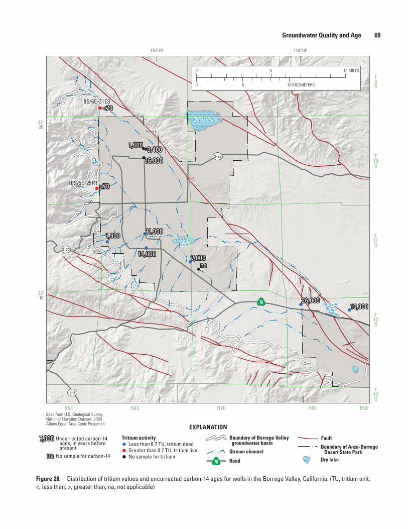
Groundwater Quality and Age 69
Figure 28. Distribution of tritium values and uncorrected carbon-14 ages for wells in the Borrego Valley, California. (TU, tritium unit; <, less than; >, greater than; na, not applicable)
Clark Lake
BorregoSink
Benson Lake
T9S
T10S
T11S
T12S
T13S
R5E R6E R7E R8E R9EBase from U.S. Geological Survey National Elevation Dataset, 2006Albers Equal Area Conic Projection
S-22
S-22
S-2
78
9S/6E-31E3
10S/5E-25R1
1,600
1,900
<70
<70
3,400
16,000
11,000
14,000
26,00010,000
7,000na
116°10’116°20’
33°20’
33°10’
0
0 5 10
5 10 MILES
KILOMETERS
sac13-0509_Figure 28 GW age
EXPLANATION
7,000Less than 0.7 TU, tritium deadGreater than 0.7 TU, tritium liveNo sample for tritium
Uncorrected carbon-14 ages, in years before present
Tritium activity
Stream channel
Boundary of Borrego Valley groundwater basin
Road78No sample for carbon-14na
Boundary of Anza-Borrego Desert State Park
Fault
Dry lake
70 Hydrogeology, Hydrologic Effects of Development, and Simulation of Groundwater Flow in the Borrego Valley
Land Subsidence
Groundwater-level declines accompanying the long-term extraction of groundwater cause an increase in the effective (intergranular) stress on the aquifer-system skeleton (matrix) that varies with respect to the distribution of hydraulic head changes in the aquifers and aquitards (interbeds and confining units) constituting the aquifer system. Depending upon the magnitude of the increased effective stress with respect to the stress history of the aquifer system, either relatively small-magnitude, reversible (elastic) or relatively larger magnitude, irreversible (inelastic) aquifer-system compaction and accompanying land subsidence can result. Aquifer-system compaction and land subsidence occur in many alluvial groundwater basins in California and elsewhere where significant quantities of water have been removed from storage in the aquifer system (Galloway and others, 1999). Two methods were employed as part of this study to assess land subsidence in Borrego Valley. In the first method, Global Positioning System (GPS) surveys were done, and continuous GPS (CGPS) data were gathered and analyzed. The GPS surveys were done in December 2008 and March 2009 to derive accurate land-surface elevations, which were compared to historical spirit-leveling data from the 1960s and 1970s. In the second method, interferometric synthetic aperture radar (InSAR) satellite remote sensing techniques were used to assess short-term (2003–07) land subsidence at a high spatial resolution over a larger area. InSAR provides spatially detailed ground-deformation maps (interferograms) that can elucidate spatially detailed patterns of vertical deformation for specific time spans (approximately months to several years or more). InSAR data complement the CGPS data, which measure deformation at high temporal frequencies over longer periods at a series of points.
Global Positioning System
The GPS is a U.S. Department of Defense satellite-based navigation system designed to provide continuous worldwide positioning and navigation capability. GNSS stands for Global Navigation Satellite System and is the standard generic term for satellite navigation systems that provide autonomous geo-spatial positioning with global coverage. This term includes GPS and is specific to the United States’ GNSS system. For this study, GPS measurements were made on geodetic monuments and reference marks (referenced to measuring points) on groundwater wells to determine their 3-D positions and to establish a geodetic or land-subsidence monitoring network (fig. 29). The modern 3-D positions of the geodetic monuments were used to determine, combined with results from historical spirit-leveling surveys, relative changes in land-surface elevations since the 1960s and 1970s. The GPS measurements also were used to establish baseline values for comparisons with results of future surveys. The 3-D positions of groundwater wells were determined for this study primarily
to improve the crude elevations derived from topographic maps on which many of the groundwater levels, and thereby much of the groundwater hydraulic gradient information, are based. Historical well elevations were corrected by more than 5 ft at 10 wells and by almost 30 ft at 1 well. The corrected elevations give a better estimate of groundwater levels and groundwater-flow directions in the valley.
The land-subsidence monitoring network consists of 25 geodetic monuments used as GPS stations spaced about 1 mile or less from each other (fig. 29). Most geodetic monuments are flat metal disks anchored in the ground or to a structure and can be used in making repeated surveying measurements of horizontal and (or) vertical positions. Historical data for monuments in the Borrego Valley were compiled from the National Oceanic and Atmospheric Administration National Geodetic Survey (formerly the U.S. Coast and Geodetic Survey) and reviewed to determine the location, timing, and quality of the vertical-control data, and suitability for GPS measurements.
Ellipsoid Heights and ElevationsGPS measurements at the 25 geodetic monuments in the
land-subsidence monitoring network and at 79 groundwater wells were made during December 1–5, 2008, and March 9–13, 2009 (table 6). Measurements were made by using one dual-frequency, full-wavelength P-code GPS receiver (Trimble 4400); one data collector (Trimble TSC1); and compact antennas (with ground plane; Trimble 33429-00) to determine horizontal coordinates and ellipsoid heights. The ellipsoid height is the vertical coordinate relative to a geodetically defined reference ellipse—the reference ellipsoid that closely approximates the Earth’s shape in the study area is the North American Datum of 1983 (NAD 83). The ellipsoid heights were converted to North American Vertical Datum of 1988 (NAVD 88) elevations by using GEOID03 (http://www.ngs.noaa.gov/GEOID/). This enabled the computation and comparison of elevation changes from historical spirit-leveling elevation measurements. The differences in the elevations were used to determine the location and magnitude of vertical land-surface changes between the previous surveys and the results from this study. Trimble Geomatics Office (version 1.63) software was used for GPS computations by making baselines and least-squares adjustments.
The GPS surveying combined static and real time kinematic (RTK) methods to obtain coordinates of the 26 monuments and the 79 wells. The RTK method is a differential measurement of one location (rover station) to another location (base station) where static, or longer term, data are concurrently collected. Accuracies of the rover station coordinates derived by differential measurements are partially dependent on accurate coordinates of the base stations. To achieve accurate coordinates of the base stations, static GPS data were collected for one location (BASE, no monument) in the 2008 survey and two locations (CL-5 and BOR33, monuments) in the 2009 survey (fig. 29). GPS
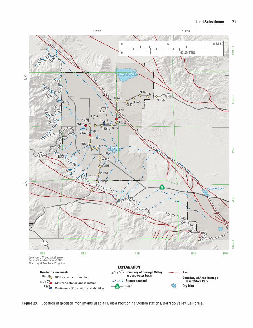
Land Subsidence 71
Clark Lake
BorregoSink
Benson Lake
T9S
T10S
T11S
T12S
T13S
R5E R6E R7E R8E R9EBase from U.S. Geological Survey National Elevation Dataset, 2006Albers Equal Area Conic Projection
S-22
S-22
S-2
78
116°10’116°20’
33°20’
33°10’
0
0 5 10
5 10 MILES
KILOMETERS
sac13-0509_Figure 29 Geo monuments
EXPLANATION
P486CL 5
CL 1
CL 33
CL 32
CL 30
Z 1326
X 1326
W 1326
V 1326
U 1326
T 1326 S 1326
R 1326
Q 1326
P 1326
N 1326
BOR 34
BOR 33BOR 12
BOR 11
BOR 10
16 JRH
15 JRH
14 JRH
11 AAR
Borregoairport
BASE
Geodetic monuments16 JRH GPS station and identifier
BOR 33 GPS base station and identifierP486 Continuous GPS station and identifier
Stream channel
Boundary of Borrego Valley groundwater basin
Road78
Boundary of Anza-Borrego Desert State Park
Fault
Dry lake
Figure 29. Location of geodetic monuments used as Global Positioning System stations, Borrego Valley, California.
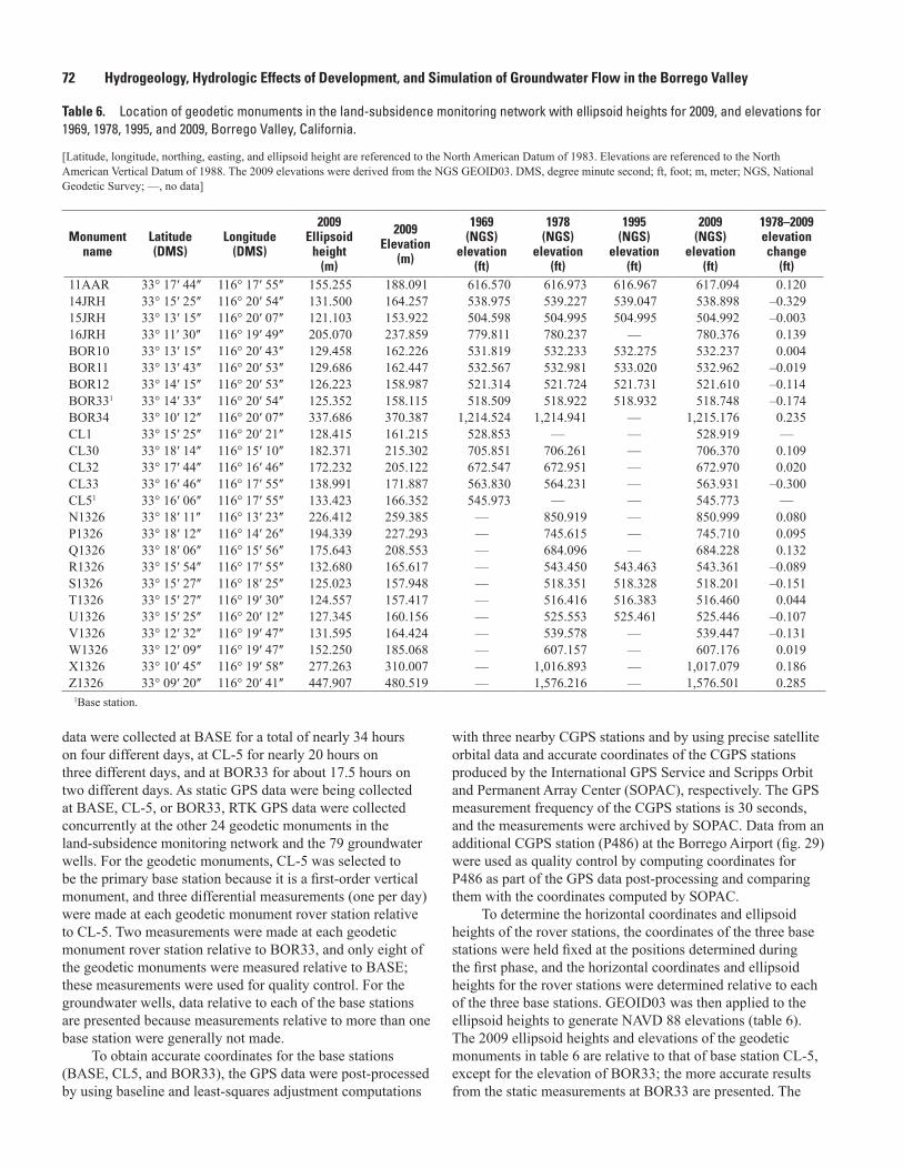
72 Hydrogeology, Hydrologic Effects of Development, and Simulation of Groundwater Flow in the Borrego Valley
data were collected at BASE for a total of nearly 34 hours on four different days, at CL-5 for nearly 20 hours on three different days, and at BOR33 for about 17.5 hours on two different days. As static GPS data were being collected at BASE, CL-5, or BOR33, RTK GPS data were collected concurrently at the other 24 geodetic monuments in the land-subsidence monitoring network and the 79 groundwater wells. For the geodetic monuments, CL-5 was selected to be the primary base station because it is a first-order vertical monument, and three differential measurements (one per day) were made at each geodetic monument rover station relative to CL-5. Two measurements were made at each geodetic monument rover station relative to BOR33, and only eight of the geodetic monuments were measured relative to BASE; these measurements were used for quality control. For the groundwater wells, data relative to each of the base stations are presented because measurements relative to more than one base station were generally not made.
To obtain accurate coordinates for the base stations (BASE, CL5, and BOR33), the GPS data were post-processed by using baseline and least-squares adjustment computations
with three nearby CGPS stations and by using precise satellite orbital data and accurate coordinates of the CGPS stations produced by the International GPS Service and Scripps Orbit and Permanent Array Center (SOPAC), respectively. The GPS measurement frequency of the CGPS stations is 30 seconds, and the measurements were archived by SOPAC. Data from an additional CGPS station (P486) at the Borrego Airport (fig. 29) were used as quality control by computing coordinates for P486 as part of the GPS data post-processing and comparing them with the coordinates computed by SOPAC.
To determine the horizontal coordinates and ellipsoid heights of the rover stations, the coordinates of the three base stations were held fixed at the positions determined during the first phase, and the horizontal coordinates and ellipsoid heights for the rover stations were determined relative to each of the three base stations. GEOID03 was then applied to the ellipsoid heights to generate NAVD 88 elevations (table 6). The 2009 ellipsoid heights and elevations of the geodetic monuments in table 6 are relative to that of base station CL-5, except for the elevation of BOR33; the more accurate results from the static measurements at BOR33 are presented. The
Table 6. Location of geodetic monuments in the land-subsidence monitoring network with ellipsoid heights for 2009, and elevations for 1969, 1978, 1995, and 2009, Borrego Valley, California.
[Latitude, longitude, northing, easting, and ellipsoid height are referenced to the North American Datum of 1983. Elevations are referenced to the North American Vertical Datum of 1988. The 2009 elevations were derived from the NGS GEOID03. DMS, degree minute second; ft, foot; m, meter; NGS, National Geodetic Survey; —, no data]
Monument name
Latitude(DMS)
Longitude(DMS)
2009Ellipsoid
height (m)
2009 Elevation
(m)
1969 (NGS)
elevation (ft)
1978 (NGS)
elevation (ft)
1995 (NGS)
elevation (ft)
2009 (NGS)
elevation (ft)
1978–2009 elevation change
(ft) 11AAR 33° 17ʹ 44ʺ 116° 17ʹ 55ʺ 155.255 188.091 616.570 616.973 616.967 617.094 0.12014JRH 33° 15ʹ 25ʺ 116° 20ʹ 54ʺ 131.500 164.257 538.975 539.227 539.047 538.898 –0.32915JRH 33° 13ʹ 15ʺ 116° 20ʹ 07ʺ 121.103 153.922 504.598 504.995 504.995 504.992 –0.00316JRH 33° 11ʹ 30ʺ 116° 19ʹ 49ʺ 205.070 237.859 779.811 780.237 — 780.376 0.139BOR10 33° 13ʹ 15ʺ 116° 20ʹ 43ʺ 129.458 162.226 531.819 532.233 532.275 532.237 0.004BOR11 33° 13ʹ 43ʺ 116° 20ʹ 53ʺ 129.686 162.447 532.567 532.981 533.020 532.962 –0.019BOR12 33° 14ʹ 15ʺ 116° 20ʹ 53ʺ 126.223 158.987 521.314 521.724 521.731 521.610 –0.114BOR331 33° 14ʹ 33ʺ 116° 20ʹ 54ʺ 125.352 158.115 518.509 518.922 518.932 518.748 –0.174BOR34 33° 10ʹ 12ʺ 116° 20ʹ 07ʺ 337.686 370.387 1,214.524 1,214.941 — 1,215.176 0.235CL1 33° 15ʹ 25ʺ 116° 20ʹ 21ʺ 128.415 161.215 528.853 — — 528.919 —CL30 33° 18ʹ 14ʺ 116° 15ʹ 10ʺ 182.371 215.302 705.851 706.261 — 706.370 0.109CL32 33° 17ʹ 44ʺ 116° 16ʹ 46ʺ 172.232 205.122 672.547 672.951 — 672.970 0.020CL33 33° 16ʹ 46ʺ 116° 17ʹ 55ʺ 138.991 171.887 563.830 564.231 — 563.931 –0.300CL51 33° 16ʹ 06ʺ 116° 17ʹ 55ʺ 133.423 166.352 545.973 — — 545.773 —N1326 33° 18ʹ 11ʺ 116° 13ʹ 23ʺ 226.412 259.385 — 850.919 — 850.999 0.080P1326 33° 18ʹ 12ʺ 116° 14ʹ 26ʺ 194.339 227.293 — 745.615 — 745.710 0.095Q1326 33° 18ʹ 06ʺ 116° 15ʹ 56ʺ 175.643 208.553 — 684.096 — 684.228 0.132R1326 33° 15ʹ 54ʺ 116° 17ʹ 55ʺ 132.680 165.617 — 543.450 543.463 543.361 –0.089S1326 33° 15ʹ 27ʺ 116° 18ʹ 25ʺ 125.023 157.948 — 518.351 518.328 518.201 –0.151T1326 33° 15ʹ 27ʺ 116° 19ʹ 30ʺ 124.557 157.417 — 516.416 516.383 516.460 0.044U1326 33° 15ʹ 25ʺ 116° 20ʹ 12ʺ 127.345 160.156 — 525.553 525.461 525.446 –0.107V1326 33° 12ʹ 32ʺ 116° 19ʹ 47ʺ 131.595 164.424 — 539.578 — 539.447 –0.131W1326 33° 12ʹ 09ʺ 116° 19ʹ 47ʺ 152.250 185.068 — 607.157 — 607.176 0.019X1326 33° 10ʹ 45ʺ 116° 19ʹ 58ʺ 277.263 310.007 — 1,016.893 — 1,017.079 0.186Z1326 33° 09ʹ 20ʺ 116° 20ʹ 41ʺ 447.907 480.519 — 1,576.216 — 1,576.501 0.285
1Base station.
Land Subsidence 73
accuracy of the geodetic-monument 2009 ellipsoid heights is plus or minus 0.5 ft at the 95-percent confidence level, which was determined by the spread of values determined from multiple GPS observations. Additionally, the error associated with elevations determined by GPS surveying could be as much as plus or minus 0.07 ft at the 95-percent confidence level because of inaccuracies in the GEOID03 model (http://www.ngs.noaa.gov/GEOID/GEOID03/tech.shtml, accessed December 4, 2009). The 2009 elevations of the groundwater wells are relative to BASE, CL-5, or BOR33 and are accurate to plus or minus 1.0 ft at the 95-percent confidence level. The groundwater-well elevations are less accurate than the geodetic monuments accuracy because repeat measurements were not made at the wells.
Land Subsidence at Geodetic MonumentsThe land-surface elevations determined from the GPS
surveys at the geodetic monuments were compared to the elevations derived from historical leveling surveys (1978–2009) to determine the magnitude of vertical land-surface changes (table 6). Generally, the comparison of monument elevations measured during surveys made at different times by different agencies with various standards of accuracy and networks of various geographic scales incorporates uncertainties of at least plus or minus 0.2 ft (Ikehara and others, 1997). As a result of various errors and because elevations in historical surveys were determined by using some elevation values that were originally referenced to the National Geodetic Vertical Datum of 1929, the uncertainty of land-surface elevation change determinations involving 2009 elevations is at least plus or minus 0.54 ft. This error was computed by applying the root sum of squares (RSS) method to the errors associated with the GPS survey (0.5 ft), the error of the geoid (0.07 ft), and the assumed errors associated with of the historical data (0.2 ft).
GPS Derived ElevationsElevations derived from GPS measurements made at
the 25 geodetic monuments in 2009 were compared with all available historical elevations, with emphasis placed on the historical elevations derived during a 1978 survey (table 6). The elevations derived from the 1978 survey were emphasized for elevation-change determinations because all but 2 of the 25 monuments (CL-1 and CL-5) were included in the 1978 survey, and more importantly, a comparison of elevations derived in 1969 and in 1978 revealed a 0.397- to 0.427-ft elevation rise for 11 of the 12 monuments that were included in both historical surveys (data for the remaining monument indicates an elevation rise of 0.253 ft). The narrow range of values of elevation rise among the 11 monuments combined with the relative stability of the monuments shown by subsequent surveys cast doubt on the accuracies of the 1969 elevations. Comparison of the 1978 elevations with the 2009 elevations indicates that the elevations of 13 monuments
increased 0.004–0.285 ft, and elevations of 10 monuments decreased 0.003–0.329 ft, during the 32-year period. For the two monuments that were not included in the 1978 survey, the comparison of the elevations derived from the 1969 and the 2009 surveys indicates that the elevation of one monument increased by 0.066 ft, and the elevation of the other monument decreased by 0.200 ft. All of the elevation changes are within the expected error of 0.54 ft; therefore, there have not been significant land-surface elevation changes at 23 monuments during the 32-year period from 1978 to 2009 or at 2 monuments during the 41-year period from 1969 to 2009.
The 3-D position of CGPS site P486 at the Borrego Airport has been continuously recorded since early 2005 and indicates about 0.787 in. of subsidence by 2010 (fig. 30). The vertical measurements both indicate a seasonal and a longer term component during 2005–10, which is not uncommon in areas where groundwater levels fluctuate seasonally. The data from this site indicated that an average net change of about 0.2 in. of subsidence occurs annually. An average of about 0.4 in. or less of subsidence occurs during the summer months, and about 0.2 in. or less of uplift occurs in the winter months, on average.
Interferometric Synthetic Aperture Radar
Interferometric synthetic aperture radar (InSAR) is a satellite-based remote sensing technique that can detect ground-surface displacement on the order of centimeters, which is an effective way to measure vertical changes of land surface over a large area between two or more specific periods. Detecting changes requires two radar images of the same area taken from approximately the same position in space, but at two different times. Comparing two synthetic aperture radar (SAR) images produces an interferogram that shows the differences in the reflected signals over an area of 0.621 by 0.621 mi (100 by 100 km). InSAR techniques have been used to investigate deformation resulting from earthquakes (Massonnet and others, 1993), volcanoes (Massonnet and others, 1995), and land subsidence (Massonnet and others, 1997; Fielding and others, 1998; Galloway and others, 1998; Amelung and others, 1999, Hoffmann and others, 2001; Sneed and others, 2001).
SAR imagery is produced by reflecting radar signals off a target area and measuring the two-way travel time back to the satellite. The SAR interferometry technique uses two SAR images of the same area acquired at different times and “interferes” (differences) them, resulting in maps called interferograms that show line-of-sight ground-surface displacement (range change) between the two periods. The generation of an interferogram produces two components: the amplitude and the phase. The amplitude component is the measure of the signal intensity returned to the satellite and shows buildings, roads, mountains, and other reflective features; the phase component is proportional to range distance and shows the coherent displacements imaged by the radar. If the ground has moved away from (subsidence)
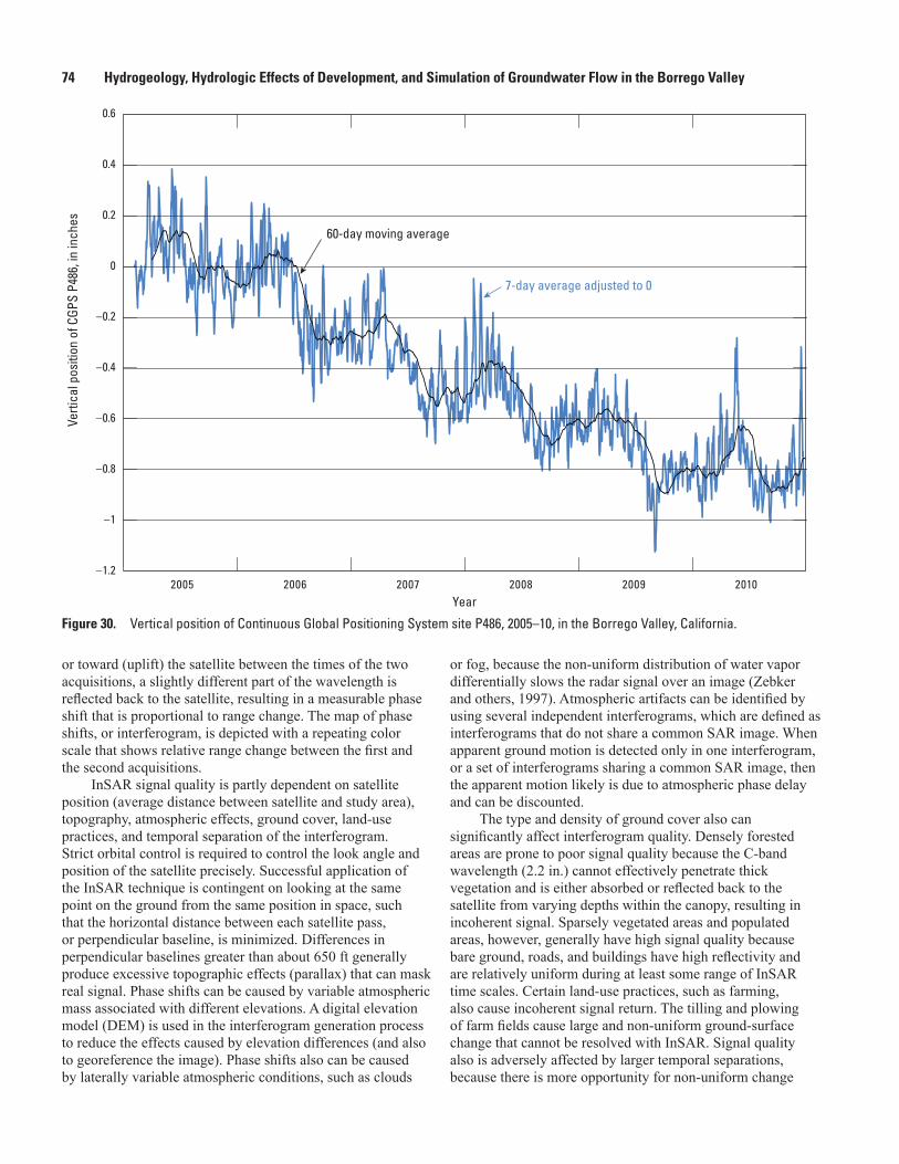
74 Hydrogeology, Hydrologic Effects of Development, and Simulation of Groundwater Flow in the Borrego Valley
sac13-0509_Figure 30 Vertical position of CGPS P486
–1.2
–1
–0.8
–0.6
–0.4
–0.2
0
0.2
0.4
0.6
7-day average adjusted to 0
Verti
cal p
ositi
on o
f CGP
S P4
86, i
n in
ches
201020092008200720062005Year
60-day moving average
Figure 30. Vertical position of Continuous Global Positioning System site P486, 2005–10, in the Borrego Valley, California.
or toward (uplift) the satellite between the times of the two acquisitions, a slightly different part of the wavelength is reflected back to the satellite, resulting in a measurable phase shift that is proportional to range change. The map of phase shifts, or interferogram, is depicted with a repeating color scale that shows relative range change between the first and the second acquisitions.
InSAR signal quality is partly dependent on satellite position (average distance between satellite and study area), topography, atmospheric effects, ground cover, land-use practices, and temporal separation of the interferogram. Strict orbital control is required to control the look angle and position of the satellite precisely. Successful application of the InSAR technique is contingent on looking at the same point on the ground from the same position in space, such that the horizontal distance between each satellite pass, or perpendicular baseline, is minimized. Differences in perpendicular baselines greater than about 650 ft generally produce excessive topographic effects (parallax) that can mask real signal. Phase shifts can be caused by variable atmospheric mass associated with different elevations. A digital elevation model (DEM) is used in the interferogram generation process to reduce the effects caused by elevation differences (and also to georeference the image). Phase shifts also can be caused by laterally variable atmospheric conditions, such as clouds
or fog, because the non-uniform distribution of water vapor differentially slows the radar signal over an image (Zebker and others, 1997). Atmospheric artifacts can be identified by using several independent interferograms, which are defined as interferograms that do not share a common SAR image. When apparent ground motion is detected only in one interferogram, or a set of interferograms sharing a common SAR image, then the apparent motion likely is due to atmospheric phase delay and can be discounted.
The type and density of ground cover also can significantly affect interferogram quality. Densely forested areas are prone to poor signal quality because the C-band wavelength (2.2 in.) cannot effectively penetrate thick vegetation and is either absorbed or reflected back to the satellite from varying depths within the canopy, resulting in incoherent signal. Sparsely vegetated areas and populated areas, however, generally have high signal quality because bare ground, roads, and buildings have high reflectivity and are relatively uniform during at least some range of InSAR time scales. Certain land-use practices, such as farming, also cause incoherent signal return. The tilling and plowing of farm fields cause large and non-uniform ground-surface change that cannot be resolved with InSAR. Signal quality also is adversely affected by larger temporal separations, because there is more opportunity for non-uniform change
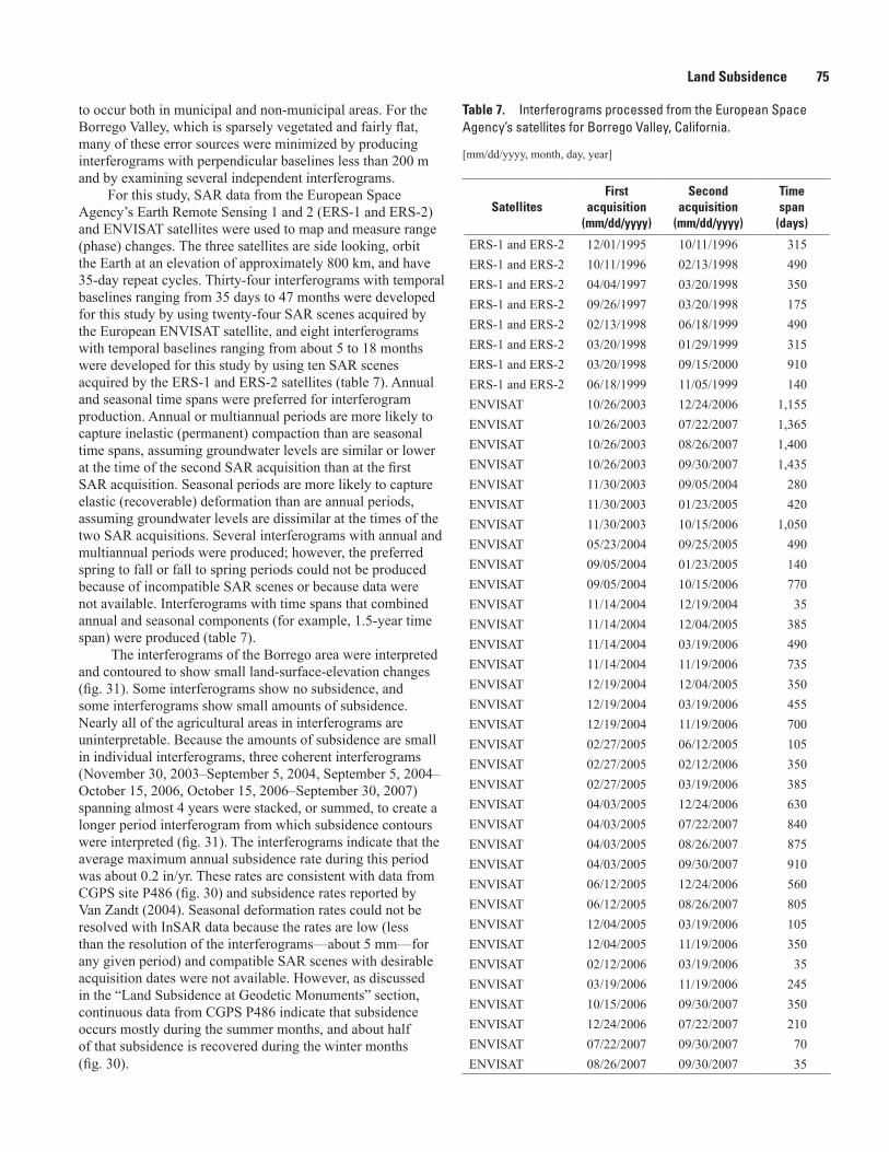
Land Subsidence 75
to occur both in municipal and non-municipal areas. For the Borrego Valley, which is sparsely vegetated and fairly flat, many of these error sources were minimized by producing interferograms with perpendicular baselines less than 200 m and by examining several independent interferograms.
For this study, SAR data from the European Space Agency’s Earth Remote Sensing 1 and 2 (ERS-1 and ERS-2) and ENVISAT satellites were used to map and measure range (phase) changes. The three satellites are side looking, orbit the Earth at an elevation of approximately 800 km, and have 35-day repeat cycles. Thirty-four interferograms with temporal baselines ranging from 35 days to 47 months were developed for this study by using twenty-four SAR scenes acquired by the European ENVISAT satellite, and eight interferograms with temporal baselines ranging from about 5 to 18 months were developed for this study by using ten SAR scenes acquired by the ERS-1 and ERS-2 satellites (table 7). Annual and seasonal time spans were preferred for interferogram production. Annual or multiannual periods are more likely to capture inelastic (permanent) compaction than are seasonal time spans, assuming groundwater levels are similar or lower at the time of the second SAR acquisition than at the first SAR acquisition. Seasonal periods are more likely to capture elastic (recoverable) deformation than are annual periods, assuming groundwater levels are dissimilar at the times of the two SAR acquisitions. Several interferograms with annual and multiannual periods were produced; however, the preferred spring to fall or fall to spring periods could not be produced because of incompatible SAR scenes or because data were not available. Interferograms with time spans that combined annual and seasonal components (for example, 1.5-year time span) were produced (table 7).
The interferograms of the Borrego area were interpreted and contoured to show small land-surface-elevation changes (fig. 31). Some interferograms show no subsidence, and some interferograms show small amounts of subsidence. Nearly all of the agricultural areas in interferograms are uninterpretable. Because the amounts of subsidence are small in individual interferograms, three coherent interferograms (November 30, 2003–September 5, 2004, September 5, 2004–October 15, 2006, October 15, 2006–September 30, 2007) spanning almost 4 years were stacked, or summed, to create a longer period interferogram from which subsidence contours were interpreted (fig. 31). The interferograms indicate that the average maximum annual subsidence rate during this period was about 0.2 in/yr. These rates are consistent with data from CGPS site P486 (fig. 30) and subsidence rates reported by Van Zandt (2004). Seasonal deformation rates could not be resolved with InSAR data because the rates are low (less than the resolution of the interferograms—about 5 mm—for any given period) and compatible SAR scenes with desirable acquisition dates were not available. However, as discussed in the “Land Subsidence at Geodetic Monuments” section, continuous data from CGPS P486 indicate that subsidence occurs mostly during the summer months, and about half of that subsidence is recovered during the winter months (fig. 30).
Table 7. Interferograms processed from the European Space Agency’s satellites for Borrego Valley, California.
[mm/dd/yyyy, month, day, year]
SatellitesFirst
acquisition(mm/dd/yyyy)
Second acquisition
(mm/dd/yyyy)
Time span
(days)
ERS-1 and ERS-2 12/01/1995 10/11/1996 315ERS-1 and ERS-2 10/11/1996 02/13/1998 490ERS-1 and ERS-2 04/04/1997 03/20/1998 350ERS-1 and ERS-2 09/26/1997 03/20/1998 175ERS-1 and ERS-2 02/13/1998 06/18/1999 490ERS-1 and ERS-2 03/20/1998 01/29/1999 315ERS-1 and ERS-2 03/20/1998 09/15/2000 910ERS-1 and ERS-2 06/18/1999 11/05/1999 140ENVISAT 10/26/2003 12/24/2006 1,155ENVISAT 10/26/2003 07/22/2007 1,365ENVISAT 10/26/2003 08/26/2007 1,400ENVISAT 10/26/2003 09/30/2007 1,435ENVISAT 11/30/2003 09/05/2004 280ENVISAT 11/30/2003 01/23/2005 420ENVISAT 11/30/2003 10/15/2006 1,050ENVISAT 05/23/2004 09/25/2005 490ENVISAT 09/05/2004 01/23/2005 140ENVISAT 09/05/2004 10/15/2006 770ENVISAT 11/14/2004 12/19/2004 35ENVISAT 11/14/2004 12/04/2005 385ENVISAT 11/14/2004 03/19/2006 490ENVISAT 11/14/2004 11/19/2006 735ENVISAT 12/19/2004 12/04/2005 350ENVISAT 12/19/2004 03/19/2006 455ENVISAT 12/19/2004 11/19/2006 700ENVISAT 02/27/2005 06/12/2005 105ENVISAT 02/27/2005 02/12/2006 350ENVISAT 02/27/2005 03/19/2006 385ENVISAT 04/03/2005 12/24/2006 630ENVISAT 04/03/2005 07/22/2007 840ENVISAT 04/03/2005 08/26/2007 875ENVISAT 04/03/2005 09/30/2007 910ENVISAT 06/12/2005 12/24/2006 560ENVISAT 06/12/2005 08/26/2007 805ENVISAT 12/04/2005 03/19/2006 105ENVISAT 12/04/2005 11/19/2006 350ENVISAT 02/12/2006 03/19/2006 35ENVISAT 03/19/2006 11/19/2006 245ENVISAT 10/15/2006 09/30/2007 350ENVISAT 12/24/2006 07/22/2007 210ENVISAT 07/22/2007 09/30/2007 70ENVISAT 08/26/2007 09/30/2007 35
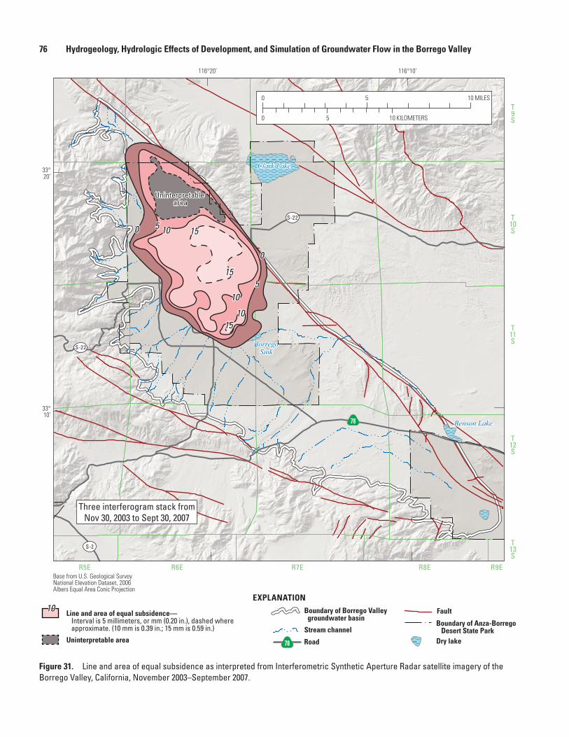
76 Hydrogeology, Hydrologic Effects of Development, and Simulation of Groundwater Flow in the Borrego Valley
Figure 31. Line and area of equal subsidence as interpreted from Interferometric Synthetic Aperture Radar satellite imagery of the Borrego Valley, California, November 2003–September 2007.
Clark Lake
BorregoSink
Benson Lake
T9S
T10S
T11S
T12S
T13S
R5E R6E R7E R8E R9EBase from U.S. Geological Survey National Elevation Dataset, 2006Albers Equal Area Conic Projection
S-22
S-22
S-2
78
Uninterpretable area
0 5 10 15
0
5
1015
10
15
116°10’116°20’
33°20’
33°10’
0
0 5 10
5 10 MILES
KILOMETERS
sac13-0509_Figure 31 InSAR subsidence
Three interferogram stack fromNov 30, 2003 to Sept 30, 2007
EXPLANATION
Line and area of equal subsidence— Interval is 5 millimeters, or mm (0.20 in.), dashed where approximate. (10 mm is 0.39 in.; 15 mm is 0.59 in.)
Uninterpretable areaStream channel
Boundary of Borrego Valley groundwater basin
Road78
10
Boundary of Anza-Borrego Desert State Park
Fault
Dry lake
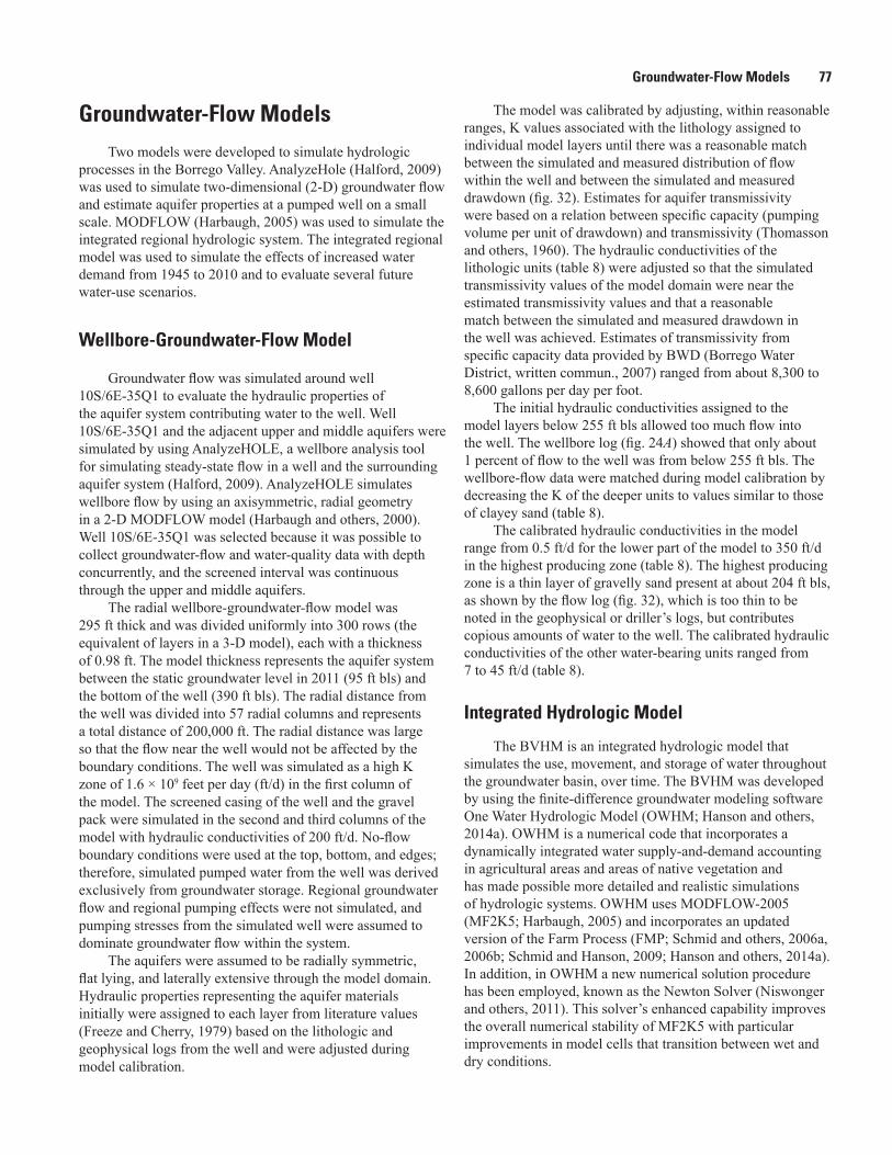
Groundwater-Flow Models 77
Groundwater-Flow ModelsTwo models were developed to simulate hydrologic
processes in the Borrego Valley. AnalyzeHole (Halford, 2009) was used to simulate two-dimensional (2-D) groundwater flow and estimate aquifer properties at a pumped well on a small scale. MODFLOW (Harbaugh, 2005) was used to simulate the integrated regional hydrologic system. The integrated regional model was used to simulate the effects of increased water demand from 1945 to 2010 and to evaluate several future water-use scenarios.
Wellbore-Groundwater-Flow Model
Groundwater flow was simulated around well 10S/6E-35Q1 to evaluate the hydraulic properties of the aquifer system contributing water to the well. Well 10S/6E-35Q1 and the adjacent upper and middle aquifers were simulated by using AnalyzeHOLE, a wellbore analysis tool for simulating steady-state flow in a well and the surrounding aquifer system (Halford, 2009). AnalyzeHOLE simulates wellbore flow by using an axisymmetric, radial geometry in a 2-D MODFLOW model (Harbaugh and others, 2000). Well 10S/6E-35Q1 was selected because it was possible to collect groundwater-flow and water-quality data with depth concurrently, and the screened interval was continuous through the upper and middle aquifers.
The radial wellbore-groundwater-flow model was 295 ft thick and was divided uniformly into 300 rows (the equivalent of layers in a 3-D model), each with a thickness of 0.98 ft. The model thickness represents the aquifer system between the static groundwater level in 2011 (95 ft bls) and the bottom of the well (390 ft bls). The radial distance from the well was divided into 57 radial columns and represents a total distance of 200,000 ft. The radial distance was large so that the flow near the well would not be affected by the boundary conditions. The well was simulated as a high K zone of 1.6 × 109 feet per day (ft/d) in the first column of the model. The screened casing of the well and the gravel pack were simulated in the second and third columns of the model with hydraulic conductivities of 200 ft/d. No-flow boundary conditions were used at the top, bottom, and edges; therefore, simulated pumped water from the well was derived exclusively from groundwater storage. Regional groundwater flow and regional pumping effects were not simulated, and pumping stresses from the simulated well were assumed to dominate groundwater flow within the system.
The aquifers were assumed to be radially symmetric, flat lying, and laterally extensive through the model domain. Hydraulic properties representing the aquifer materials initially were assigned to each layer from literature values (Freeze and Cherry, 1979) based on the lithologic and geophysical logs from the well and were adjusted during model calibration.
The model was calibrated by adjusting, within reasonable ranges, K values associated with the lithology assigned to individual model layers until there was a reasonable match between the simulated and measured distribution of flow within the well and between the simulated and measured drawdown (fig. 32). Estimates for aquifer transmissivity were based on a relation between specific capacity (pumping volume per unit of drawdown) and transmissivity (Thomasson and others, 1960). The hydraulic conductivities of the lithologic units (table 8) were adjusted so that the simulated transmissivity values of the model domain were near the estimated transmissivity values and that a reasonable match between the simulated and measured drawdown in the well was achieved. Estimates of transmissivity from specific capacity data provided by BWD (Borrego Water District, written commun., 2007) ranged from about 8,300 to 8,600 gallons per day per foot.
The initial hydraulic conductivities assigned to the model layers below 255 ft bls allowed too much flow into the well. The wellbore log (fig. 24A) showed that only about 1 percent of flow to the well was from below 255 ft bls. The wellbore-flow data were matched during model calibration by decreasing the K of the deeper units to values similar to those of clayey sand (table 8).
The calibrated hydraulic conductivities in the model range from 0.5 ft/d for the lower part of the model to 350 ft/d in the highest producing zone (table 8). The highest producing zone is a thin layer of gravelly sand present at about 204 ft bls, as shown by the flow log (fig. 32), which is too thin to be noted in the geophysical or driller’s logs, but contributes copious amounts of water to the well. The calibrated hydraulic conductivities of the other water-bearing units ranged from 7 to 45 ft/d (table 8).
Integrated Hydrologic Model
The BVHM is an integrated hydrologic model that simulates the use, movement, and storage of water throughout the groundwater basin, over time. The BVHM was developed by using the finite-difference groundwater modeling software One Water Hydrologic Model (OWHM; Hanson and others, 2014a). OWHM is a numerical code that incorporates a dynamically integrated water supply-and-demand accounting in agricultural areas and areas of native vegetation and has made possible more detailed and realistic simulations of hydrologic systems. OWHM uses MODFLOW-2005 (MF2K5; Harbaugh, 2005) and incorporates an updated version of the Farm Process (FMP; Schmid and others, 2006a, 2006b; Schmid and Hanson, 2009; Hanson and others, 2014a). In addition, in OWHM a new numerical solution procedure has been employed, known as the Newton Solver (Niswonger and others, 2011). This solver’s enhanced capability improves the overall numerical stability of MF2K5 with particular improvements in model cells that transition between wet and dry conditions.
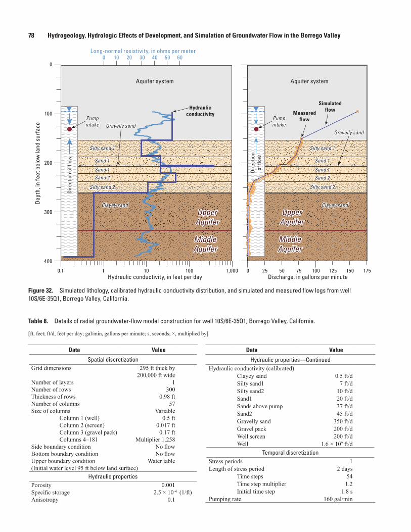
78 Hydrogeology, Hydrologic Effects of Development, and Simulation of Groundwater Flow in the Borrego ValleyD
epth
, in
feet
bel
ow la
nd s
urfa
ce
00.1 1 10 100 1,000
0
100
200
300
400
25 50 75 100Discharge, in gallons per minuteHydraulic conductivity, in feet per day
125 150 175
Pumpintake
Dire
ctio
n of
flow
Dire
ctio
nof
flow
Silty sand 1
Silty sand 2
Sand 1
Gravelly sand
Sand 1Sand 2
Clayey sand
Pumpintake
Silty sand 1
Silty sand 2
Sand 1
Gravelly sand
Sand 1Sand 2
Clayey sand
Hydraulicconductivity Measured
flow
Simulatedflow
Aquifer system Aquifer system
sac13-0509_Figure 32 MV-4 logs simulated
0 10 20 30 40 50 60Long-normal resistivity, in ohms per meter
UpperAquifer
MiddleAquifer
UpperAquifer
MiddleAquifer
Figure 32. Simulated lithology, calibrated hydraulic conductivity distribution, and simulated and measured flow logs from well 10S/6E-35Q1, Borrego Valley, California.
Table 8. Details of radial groundwater-flow model construction for well 10S/6E-35Q1, Borrego Valley, California.
[ft, feet; ft/d, feet per day; gal/min, gallons per minute; s, seconds; ×, multiplied by]
Data Value
Spatial discretizationGrid dimensions 295 ft thick by
200,000 ft wideNumber of layers 1Number of rows 300Thickness of rows 0.98 ftNumber of columns 57Size of columns Variable
Column 1 (well) 0.5 ftColumn 2 (screen) 0.017 ftColumn 3 (gravel pack) 0.17 ftColumns 4–181 Multiplier 1.258
Side boundary condition No flowBottom boundary condition No flowUpper boundary condition Water table(Initial water level 95 ft below land surface)
Hydraulic propertiesPorosity 0.001Specific storage 2.5 × 10⁻⁶ (1/ft)Anisotropy 0.1
Data Value
Hydraulic properties—ContinuedHydraulic conductivity (calibrated)
Clayey sand 0.5 ft/dSilty sand1 7 ft/dSilty sand2 10 ft/dSand1 20 ft/dSands above pump 37 ft/dSand2 45 ft/dGravelly sand 350 ft/dGravel pack 200 ft/dWell screen 200 ft/dWell 1.6 × 109 ft/d
Temporal discretizationStress periods 1Length of stress period 2 days
Time steps 54Time step multiplier 1.2Initial time step 1.8 s
Pumping rate 160 gal/min
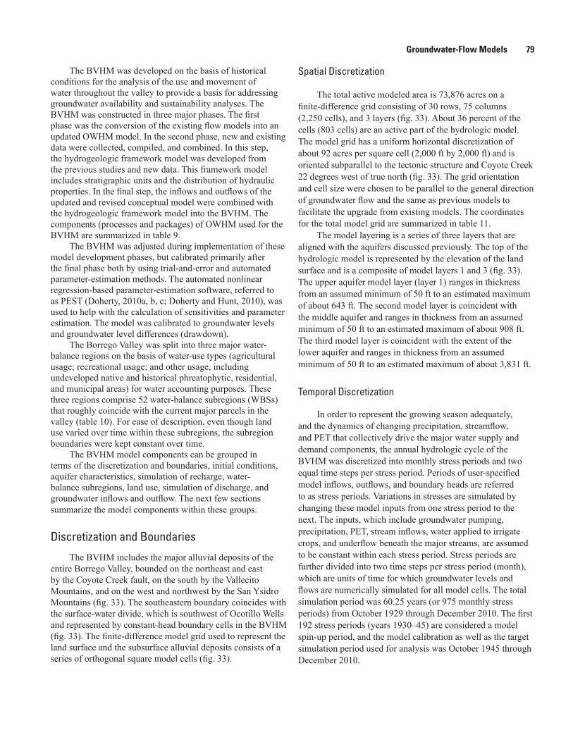
Groundwater-Flow Models 79
Spatial Discretization
The total active modeled area is 73,876 acres on a finite-difference grid consisting of 30 rows, 75 columns (2,250 cells), and 3 layers (fig. 33). About 36 percent of the cells (803 cells) are an active part of the hydrologic model. The model grid has a uniform horizontal discretization of about 92 acres per square cell (2,000 ft by 2,000 ft) and is oriented subparallel to the tectonic structure and Coyote Creek 22 degrees west of true north (fig. 33). The grid orientation and cell size were chosen to be parallel to the general direction of groundwater flow and the same as previous models to facilitate the upgrade from existing models. The coordinates for the total model grid are summarized in table 11.
The model layering is a series of three layers that are aligned with the aquifers discussed previously. The top of the hydrologic model is represented by the elevation of the land surface and is a composite of model layers 1 and 3 (fig. 33). The upper aquifer model layer (layer 1) ranges in thickness from an assumed minimum of 50 ft to an estimated maximum of about 643 ft. The second model layer is coincident with the middle aquifer and ranges in thickness from an assumed minimum of 50 ft to an estimated maximum of about 908 ft. The third model layer is coincident with the extent of the lower aquifer and ranges in thickness from an assumed minimum of 50 ft to an estimated maximum of about 3,831 ft.
Temporal Discretization
In order to represent the growing season adequately, and the dynamics of changing precipitation, streamflow, and PET that collectively drive the major water supply and demand components, the annual hydrologic cycle of the BVHM was discretized into monthly stress periods and two equal time steps per stress period. Periods of user-specified model inflows, outflows, and boundary heads are referred to as stress periods. Variations in stresses are simulated by changing these model inputs from one stress period to the next. The inputs, which include groundwater pumping, precipitation, PET, stream inflows, water applied to irrigate crops, and underflow beneath the major streams, are assumed to be constant within each stress period. Stress periods are further divided into two time steps per stress period (month), which are units of time for which groundwater levels and flows are numerically simulated for all model cells. The total simulation period was 60.25 years (or 975 monthly stress periods) from October 1929 through December 2010. The first 192 stress periods (years 1930–45) are considered a model spin-up period, and the model calibration as well as the target simulation period used for analysis was October 1945 through December 2010.
The BVHM was developed on the basis of historical conditions for the analysis of the use and movement of water throughout the valley to provide a basis for addressing groundwater availability and sustainability analyses. The BVHM was constructed in three major phases. The first phase was the conversion of the existing flow models into an updated OWHM model. In the second phase, new and existing data were collected, compiled, and combined. In this step, the hydrogeologic framework model was developed from the previous studies and new data. This framework model includes stratigraphic units and the distribution of hydraulic properties. In the final step, the inflows and outflows of the updated and revised conceptual model were combined with the hydrogeologic framework model into the BVHM. The components (processes and packages) of OWHM used for the BVHM are summarized in table 9.
The BVHM was adjusted during implementation of these model development phases, but calibrated primarily after the final phase both by using trial-and-error and automated parameter-estimation methods. The automated nonlinear regression-based parameter-estimation software, referred to as PEST (Doherty, 2010a, b, c; Doherty and Hunt, 2010), was used to help with the calculation of sensitivities and parameter estimation. The model was calibrated to groundwater levels and groundwater level differences (drawdown).
The Borrego Valley was split into three major water-balance regions on the basis of water-use types (agricultural usage; recreational usage; and other usage, including undeveloped native and historical phreatophytic, residential, and municipal areas) for water accounting purposes. These three regions comprise 52 water-balance subregions (WBSs) that roughly coincide with the current major parcels in the valley (table 10). For ease of description, even though land use varied over time within these subregions, the subregion boundaries were kept constant over time.
The BVHM model components can be grouped in terms of the discretization and boundaries, initial conditions, aquifer characteristics, simulation of recharge, water-balance subregions, land use, simulation of discharge, and groundwater inflows and outflow. The next few sections summarize the model components within these groups.
Discretization and Boundaries
The BVHM includes the major alluvial deposits of the entire Borrego Valley, bounded on the northeast and east by the Coyote Creek fault, on the south by the Vallecito Mountains, and on the west and northwest by the San Ysidro Mountains (fig. 33). The southeastern boundary coincides with the surface-water divide, which is southwest of Ocotillo Wells and represented by constant-head boundary cells in the BVHM (fig. 33). The finite-difference model grid used to represent the land surface and the subsurface alluvial deposits consists of a series of orthogonal square model cells (fig. 33).
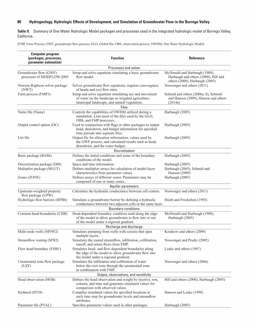
80 Hydrogeology, Hydrologic Effects of Development, and Simulation of Groundwater Flow in the Borrego Valley
Table 9. Summary of One Water Hydrologic Model packages and processes used in the integrated hydrologic model of Borrego Valley, California.
[FMP, Farm Process; GWF, groundwater flow process; GLO, Global file; OBS, observation process; OWHM, One Water Hydrologic Model]
Computer program (packages, processes, parameter estimation)
Function Reference
Processes and solverGroundwater flow (GWF)
processes of MODFLOW-2005Setup and solve equations simulating a basic groundwater
flow model.McDonald and Harbaugh (1988),
Harbaugh and others (2000), Hill and others (2000), Harbaugh (2005)
Newton-Raphson solver package (NWT)
Solves groundwater flow equations; requires convergence of heads and (or) flow rates.
Niswonger and others (2011)
Farm process (FMP3) Setup and solve equations simulating use and movement of water on the landscape as irrigated agriculture, municipal landscape, and natural vegetation.
Schmid and others (2006a, b), Schmid and Hanson (2009), Hanson and others (2014a)
FilesName file (Name) Controls the capabilities of OWHM utilized during a
simulation. Lists most of the files used by the GLO, OBS, and FMP processes.
Harbaugh (2005)
Output control option (OC) Used in conjunction with flags in other packages to output head, drawdown, and budget information for specified time periods into separate files.
Harbaugh (2005)
List file Output file for allocation information, values used by the GWF process, and calculated results such as head, drawdown, and the water budget.
Harbaugh (2005)
Discretization Basic package (BAS6) Defines the initial conditions and some of the boundary
conditions of the model.Harbaugh (2005)
Discretization package (DIS) Space and time information. Harbaugh (2005)Multiplier package (MULT) Defines multiplier arrays for calculation of model-layer
characteristics from parameter values.Harbaugh (2005), Schmid and
Hanson (2009)Zones (ZONE) Defines arrays of different zones. Parameters may be
composed of one or many zones.Harbaugh (2005)
Aquifer parametersUpstream-weighted property
flow package (UPW)Calculates the hydraulic conductance between cell centers. Niswonger and others (2011)
Hydrologic flow barriers (HFB6) Simulates a groundwater barrier by defining a hydraulic conductance between two adjacent cells in the same layer.
Hsieh and Freckelton (1993)
Boundary conditionsConstant head boundaries (CHB) Head-dependent boundary condition used along the edge
of the model to allow groundwater to flow into or out of the model under a regional gradient.
McDonald and Harbaugh (1988), Harbaugh (2005)
Recharge and dischargeMulti-node wells (MNW2) Simulates pumping from wells with screens that span
multiple layers.Konikow and others (2009)
Streamflow routing (SFR2) Simulates the routed streamflow, infiltration, exfiltration, runoff, and return flows from FMP.
Niswonger and Prudic (2005)
Flow head boundary (FHB1) Simulates head- and flow-dependent boundaries along the edge of the model to allow groundwater flow into the model under a regional gradient.
Leake and others (1997)
Unsaturated zone flow package (UZF)
Simulates the infiltration and exfiltration of water below the root zone through the unsaturated zone in combination with FMP.
Niswonger and others (2006)
Output, observations, and sensitivityHead observation (HOB) Defines the head observation and weight by layer(s), row,
column, and time and generates simulated values for comparison with observed values.
Hill and others (2000), Harbaugh (2005)
Hydmod (HYD) Compiles simulated values for specified locations at each time step for groundwater levels and streamflow attributes.
Hanson and Leake (1998)
Parameter file (PVAL) Specifies parameter values used in other packages. Harbaugh (2005)
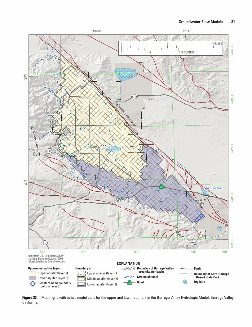
Groundwater-Flow Models 81
Vallecito Mountains
Clark Lake
BorregoSink
Benson Lake
T9S
T10S
T11S
T12S
T13S
R5E R6E R7E R8E R9EBase from U.S. Geological Survey National Elevation Dataset, 2006Albers Equal Area Conic Projection
S-22
S-22
S-2
78
116°10’116°20’
33°20’
33°10’
0
0 5 10
5 10 MILES
KILOMETERS
sac13-0509_Figure 33_Upper active layer
EXPLANATION
Ocotillowells
Upper-most active layer Boundary of
Constant-head boundary cells in layer 3
Upper aquifer (layer 1)Lower aquifer (layer 3)
Upper aquifer (layer 1)
Middle aquifer (layer 2)
Lower aquifer (layer 3)
Stream channel
Boundary of Borrego Valley groundwater basin
Road78
Boundary of Anza-Borrego Desert State Park
Fault
Dry lake
San Ysidro M
ountains
Coyote Creek fault
Figure 33. Model grid with active model cells for the upper and lower aquifers in the Borrego Valley Hydrologic Model, Borrego Valley, California.
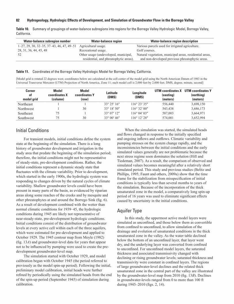
82 Hydrogeology, Hydrologic Effects of Development, and Simulation of Groundwater Flow in the Borrego Valley
Initial Conditions
For transient models, initial conditions define the system state at the beginning of the simulation. There is a long history of groundwater development and irrigation in the study area that predate the beginning of the simulation period; therefore, the initial conditions might not be representative of steady-state, pre-development conditions. Rather, the initial conditions represent a dynamic steady state that fluctuates with the climate variability. Prior to development, which started in the early 1900s, the hydrologic system was responding to changes driven by the natural cycles of climate variability. Shallow groundwater levels could have been present in many parts of the basin, as evidenced by riparian areas along some reaches of the creeks and by mesquite and other phreatophytes at and around the Borrego Sink (fig. 6). As a result of development combined with the wetter than normal climatic conditions for 1939–45, the hydrologic conditions during 1945 are likely not representative of near-steady-state, pre-development hydrologic conditions. Initial conditions consist of the distribution of groundwater levels at every active cell within each of the three aquifers, which were estimated for pre-development and applied to October 1929. The 1945 contour map from Moyle (1982) (fig. 13A) and groundwater-level data for years that appear not to be influenced by pumping were used to create the pre-development groundwater-level map.
The simulation started with October 1929, and model calibration began with October 1945 (the period referred to previously as the model spin-up period). Following the initial, preliminary model calibration, initial heads were further refined by periodically using the simulated heads from the end of the spin-up period (September 1945) of simulation during calibration.
When the simulation was started, the simulated heads and flows changed in response to the initially specified and ongoing inflows and outflows. Climatic variability and pumping stresses on the system change rapidly, and the inconsistencies between the initial conditions and the early simulated values generally are not problematic because the next stress regime soon dominates the solution (Hill and Tiedeman, 2007). As a result, the comparison of observed and simulated values becomes meaningful after a relatively short simulated period. This study and previous studies (Belitz and Phillips, 1995; Faunt and others, 2009a) show that the time frame for the stabilization from misspecification of initial conditions is typically less than several months to years of the simulation. Because of the incorporation of the thick unsaturated zone in the model, a comparatively long spin-up period of 16 years was used to eliminate significant effects caused by uncertainty in the initial conditions.
Aquifer TypeIn this study, the uppermost active model layers were
simulated as unconfined, and those below them as convertible from confined to unconfined, to allow simulation of the drainage and evolution of unsaturated conditions in the thick unsaturated zone in the valley. As the water table declined below the bottom of an unconfined layer, that layer went dry, and the underlying layer was converted from confined to unconfined. For unconfined model layers, the saturated thickness and associated transmissivity changed with declining or rising groundwater levels; saturated thickness and transmissivity were constant in confined layers. The regions of large groundwater-level declines and the related thick unsaturated zone in the central part of the valley are illustrated by the groundwater-level map from 2010 (fig. 13B). Declines in groundwater-levels ranged from 0 to more than 100 ft during 1945–2010 (figs. 2, 14).
Table 10. Summary of groupings of water-balance subregions into regions for the Borrego Valley Hydrologic Model, Borrego Valley, California.
Water-balance subregion number Water-balance region Water-balance region description1–27, 29, 30, 32–35, 37–43, 46, 47, 49–51 Agricultural usage. Various parcels used for irrigated agriculture.28, 31, 36, 44, 45, 48 Recreational usage. Golf courses.52 Other usage (undeveloped, municipal,
residential, and phreatophytic areas).Natural vegetation, municipal areas, residential areas,
and non-developed previous phreatophytic areas.
Table 11. Coordinates of the Borrego Valley Hydrologic Model for Borrego Valley, California.
[Model grid is rotated 22 degrees west; coordinates below are calculated at the cell center of the model grid using the North American Datum of 1983 in the Universal Transverse Mercator (UTM) Projection of North America, Zone 11; each model cell is 2,000 feet by 2,000 feet. DMS, degree, minute, second]
Corner of
model grid
Model coordinates X
(column)
Model coordinates Y
(row)
Latitude (DMS)
Longitude (DMS)
UTM coordinates X (easting) (meters)
UTM coordinates Y (northing) (meters)
Northeast 1 1 33° 25ʹ 16ʺ 116° 23ʹ 35ʺ 556,440 3,698,150Northwest 1 30 33° 18ʹ 50ʺ 116° 32ʹ 00ʺ 543,438 3,686,173Southeast 75 1 33° 07ʹ 12ʺ 116° 04ʹ 03ʺ 587,003 3,664,971Southwest 75 30 33° 00ʹ 46ʺ 116° 12ʹ 28ʺ 574,001 3,652,994
Groundwater-Flow Models 83
Aquifer CharacteristicsThe Borrego Valley has three aquifers that can be
characterized by variations in hydraulic properties based on the textural distribution of coarse- and fine-grained sediments and zones that represent sediments derived from particular depositional environments (figs. 12, 34). The hydraulic properties represent the ability of the aquifer to transmit water and to store or release water; hydraulic properties differ according to grain size and the degree of sorting of the sediments, which are functions of lithology and depositional environment. Thus, considerable spatial variation exists in the hydraulic properties of the heterogeneous aquifer system. The hydraulic water-transmitting properties of the aquifer sediments are represented by their horizontal (Kh) and vertical (Kv) hydraulic conductivities. The hydraulic storage properties both include the properties of the aquifers and any fine-grained interbeds or confining units. Storage properties of the unconfined model layers are represented by the specific yield and specific storage in the confined model layers (see “Storage Properties” section). The relation between hydrogeologic units, lithology, sediment texture, and hydraulic properties has been described in many previous studies (Laudon and Belitz, 1991; Phillips and Belitz, 1991; Leighton and others, 1994; Fio and Leighton, 1995; Belitz and Phillips, 1995; Burow and others, 2004, and Phillips and others, 2007; Faunt and others, 2009a, 2009b; Sweetkind and others, 2013).
Textural AnalysisHeterogeneity, lateral and vertical variation in sediment
texture and related hydrogeologic properties, affects the direction and rate of groundwater flow, as well as the magnitude and distribution of aquifer-system storativity. The textural distribution was used to define the Kh and Kv and storage property distributions for the hydrologic model. As in many of the previous studies identified, this textural distribution was based on drillers’ and geophysical logs. The primary variable selected for the textural analysis was the percentage of coarse-grained sediments, with the complement being the percentage of fine-grained sediments.
As described earlier, the distribution of sediment texture in the three aquifers of the Borrego Valley aquifer system was based on a reanalysis of the hydrogeology. In the model, within each aquifer, the fraction of coarse- and fine-grained sediments within the thickness of each aquifer model layer was estimated on a cell-by-cell basis (fig. 12). Texture was estimated at the cell centers of the model grid for each of the aquifers.
Calculation of Hydraulic PropertiesTextural-based estimates of hydraulic properties were
made separately for each of the three aquifers. The hydraulic properties of an aquifer are its transmission and storage properties. The transmission properties of the Borrego Valley aquifer are represented by the K in this study. Equivalent Kh
and Kvs are assumed to be correlated to sediment texture (the fraction of coarse-grained and fine-grained sediment). The K was calculated by using the estimated binary sediment texture for each model cell and Kh and Kv estimates for each textural end member (coarse and fine).
Separate methods were used to calculate estimates for horizontal and vertical hydraulic conductivities. The Kh (Kh,i) was calculated as the weighted arithmetic mean of the hydraulic conductivities of the coarse-grained (Kc ) and fine-grained (Kf ) lithologic end members and the distribution of sediment texture for each model cell i:
Kh,i = + K F K Fc c i f f i, , (2)
where Fc,i is the fraction of coarse-grained sediment in a
cell, estimated from sediment texture data as described in the previous section, and
Ff,i is the fraction of fine-grained sediment in a cell (1 – Fc,i).
Because Kf is much smaller than Kc, the arithmetic mean heavily weights the coarse-grained end member for Kh.
Faunt and others (2009a) identify the power mean as useful for defining Kv values. In addition, their work also includes a review of the literature that describes the use of the power mean for estimating K. A power mean is given by the following equation:
M x
nxpkp
k
n p
( ) =
=
∑11
1
(3)
where p is the averaging power-mean exponent, n is the number of elements being averaged, and Xk is the kth element in the list.
The Kv between model layers ( Kv k, + 12) was calculated as
the pth weighted power mean of the hydraulic conductivities of the coarse- and fine-grained lithologic end members (Faunt and others, 2009a):
K F K F Kv k c k c
pf k f
p p
, , ,+ + += +
1
21
21
2
1
(4)
where
Fc k, + 1
2 is the fraction of coarse-grained sediment between layer midpoints, and
Ff k, + 1
2 is the fraction of fine-grained sediment between layer midpoints.
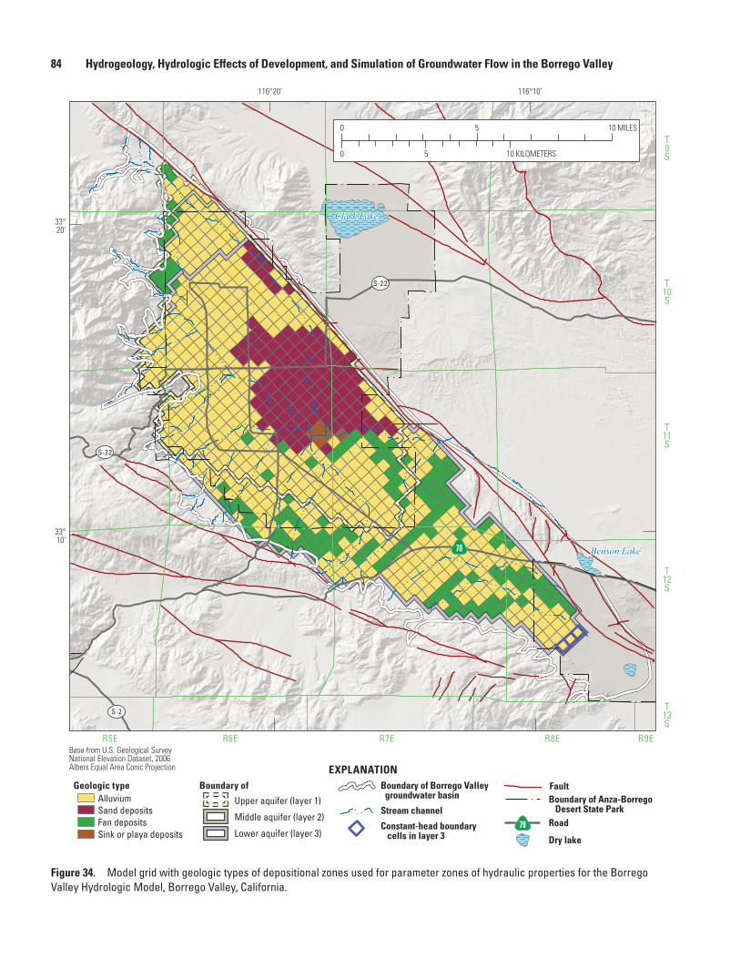
84 Hydrogeology, Hydrologic Effects of Development, and Simulation of Groundwater Flow in the Borrego Valley
Clark Lake
Benson Lake
T9S
T10S
T11S
T12S
T13S
R5E R6E R7E R8E R9EBase from U.S. Geological Survey National Elevation Dataset, 2006Albers Equal Area Conic Projection
S-22
S-22
S-2
78
116°10’116°20’
33°20’
33°10’
0
0 5 10
5 10 MILES
KILOMETERS
sac13-0509_Figure 34_Hk zones
EXPLANATION
AlluviumSand depositsFan depositsSink or playa deposits
Constant-head boundary cells in layer 3
Geologic type Boundary of
Stream channel
Boundary of Borrego Valley groundwater basinUpper aquifer (layer 1)
Middle aquifer (layer 2)
Lower aquifer (layer 3)
Boundary of Anza-Borrego Desert State Park
Fault
Road78
Dry lake
Figure 34. Model grid with geologic types of depositional zones used for parameter zones of hydraulic properties for the Borrego Valley Hydrologic Model, Borrego Valley, California.
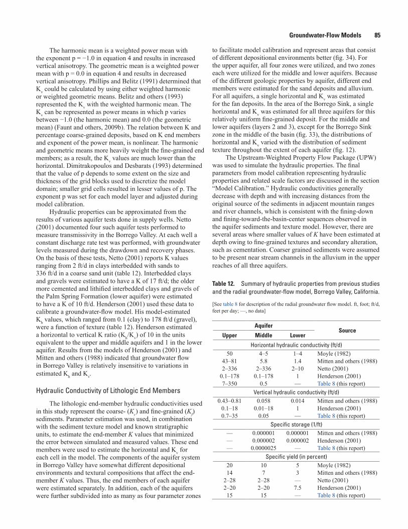
Groundwater-Flow Models 85
The harmonic mean is a weighted power mean with the exponent p = −1.0 in equation 4 and results in increased vertical anisotropy. The geometric mean is a weighted power mean with p = 0.0 in equation 4 and results in decreased vertical anisotropy. Phillips and Belitz (1991) determined that Kv could be calculated by using either weighted harmonic or weighted geometric means. Belitz and others (1993) represented the Kv with the weighted harmonic mean. The Kv can be represented as power means in which p varies between −1.0 (the harmonic mean) and 0.0 (the geometric mean) (Faunt and others, 2009b). The relation between K and percentage coarse-grained deposits, based on K end members and exponent of the power mean, is nonlinear. The harmonic and geometric means more heavily weight the fine-grained end members; as a result, the Kv values are much lower than the horizontal. Dimitrakopoulos and Desbarats (1993) determined that the value of p depends to some extent on the size and thickness of the grid blocks used to discretize the model domain; smaller grid cells resulted in lesser values of p. The exponent p was set for each model layer and adjusted during model calibration.
Hydraulic properties can be approximated from the results of various aquifer tests done in supply wells. Netto (2001) documented four such aquifer tests performed to measure transmissivity in the Borrego Valley. At each well a constant discharge rate test was performed, with groundwater levels measured during the drawdown and recovery phases. On the basis of these tests, Netto (2001) reports K values ranging from 2 ft/d in clays interbedded with sands to 336 ft/d in a coarse sand unit (table 12). Interbedded clays and gravels were estimated to have a K of 17 ft/d; the older more cemented and lithified interbedded clays and gravels of the Palm Spring Formation (lower aquifer) were estimated to have a K of 10 ft/d. Henderson (2001) used these data to calibrate a groundwater-flow model. His model-estimated Kh values, which ranged from 0.1 (clay) to 178 ft/d (gravel), were a function of texture (table 12). Henderson estimated a horizontal to vertical K ratio (Kh/Kv) of 10 in the units equivalent to the upper and middle aquifers and 1 in the lower aquifer. Results from the models of Henderson (2001) and Mitten and others (1988) indicated that groundwater flow in Borrego Valley is relatively insensitive to variations in estimated Kh and Kv.
Hydraulic Conductivity of Lithologic End Members
The lithologic end-member hydraulic conductivities used in this study represent the coarse- (Kc) and fine-grained (Kf) sediments. Parameter estimation was used, in combination with the sediment texture model and known stratigraphic units, to estimate the end-member K values that minimized the error between simulated and measured values. These end members were used to estimate the horizontal and Kv for each cell in the model. The components of the aquifer system in Borrego Valley have somewhat different depositional environments and textural compositions that affect the end-member K values. Thus, the end members of each aquifer were estimated separately. In addition, each of the aquifers were further subdivided into as many as four parameter zones
to facilitate model calibration and represent areas that consist of different depositional environments better (fig. 34). For the upper aquifer, all four zones were utilized, and two zones each were utilized for the middle and lower aquifers. Because of the different geologic properties by aquifer, different end members were estimated for the sand deposits and alluvium. For all aquifers, a single horizontal and Kv was estimated for the fan deposits. In the area of the Borrego Sink, a single horizontal and Kv was estimated for all three aquifers for this relatively uniform fine-grained deposit. For the middle and lower aquifers (layers 2 and 3), except for the Borrego Sink zone in the middle of the basin (fig. 33), the distributions of horizontal and Kv varied with the distribution of sediment texture throughout the extent of each aquifer (fig. 12).
The Upstream-Weighted Property Flow Package (UPW) was used to simulate the hydraulic properties. The final parameters from model calibration representing hydraulic properties and related scale factors are discussed in the section “Model Calibration.” Hydraulic conductivities generally decrease with depth and with increasing distances from the original source of the sediments in adjacent mountain ranges and river channels, which is consistent with the fining-down and fining-toward-the-basin-center sequences observed in the aquifer sediments and texture model. However, there are several areas where smaller values of K have been estimated at depth owing to fine-grained textures and secondary alteration, such as cementation. Coarser grained sediments were assumed to be present near stream channels in the alluvium in the upper reaches of all three aquifers.
Table 12. Summary of hydraulic properties from previous studies and the radial groundwater-flow model, Borrego Valley, California.
[See table 8 for description of the radial groundwater flow model. ft, foot; ft/d, feet per day; —, no data]
AquiferSource
Upper Middle Lower
Horizontal hydraulic conductivity (ft/d)50 4–5 1–4 Moyle (1982)
43–81 5.8 1.4 Mitten and others (1988) 2–336 2–336 2–10 Netto (2001)
0.1–178 0.1–178 1 Henderson (2001)7–350 0.5 — Table 8 (this report)
Vertical hydraulic conductivity (ft/d)0.43–0.81 0.058 0.014 Mitten and others (1988)
0.1–18 0.01–18 1 Henderson (2001)0.7–35 0.05 — Table 8 (this report)
Specific storage (1/ft)— 0.000001 0.000001 Mitten and others (1988) — 0.000002 0.000002 Henderson (2001)— 0.0000025 — Table 8 (this report)
Specific yield (in percent)20 10 5 Moyle (1982)14 7 3 Mitten and others (1988)
2–28 2–28 — Netto (2001)2–20 2–20 7.5 Henderson (2001)15 15 — Table 8 (this report)
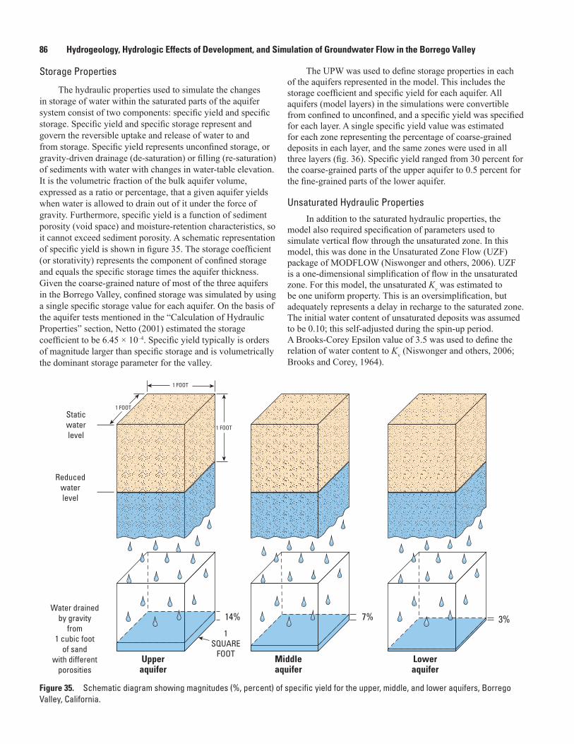
86 Hydrogeology, Hydrologic Effects of Development, and Simulation of Groundwater Flow in the Borrego Valley
Storage Properties
The hydraulic properties used to simulate the changes in storage of water within the saturated parts of the aquifer system consist of two components: specific yield and specific storage. Specific yield and specific storage represent and govern the reversible uptake and release of water to and from storage. Specific yield represents unconfined storage, or gravity-driven drainage (de-saturation) or filling (re-saturation) of sediments with water with changes in water-table elevation. It is the volumetric fraction of the bulk aquifer volume, expressed as a ratio or percentage, that a given aquifer yields when water is allowed to drain out of it under the force of gravity. Furthermore, specific yield is a function of sediment porosity (void space) and moisture-retention characteristics, so it cannot exceed sediment porosity. A schematic representation of specific yield is shown in figure 35. The storage coefficient (or storativity) represents the component of confined storage and equals the specific storage times the aquifer thickness. Given the coarse-grained nature of most of the three aquifers in the Borrego Valley, confined storage was simulated by using a single specific storage value for each aquifer. On the basis of the aquifer tests mentioned in the “Calculation of Hydraulic Properties” section, Netto (2001) estimated the storage coefficient to be 6.45 × 10⁻⁴. Specific yield typically is orders of magnitude larger than specific storage and is volumetrically the dominant storage parameter for the valley.
The UPW was used to define storage properties in each of the aquifers represented in the model. This includes the storage coefficient and specific yield for each aquifer. All aquifers (model layers) in the simulations were convertible from confined to unconfined, and a specific yield was specified for each layer. A single specific yield value was estimated for each zone representing the percentage of coarse-grained deposits in each layer, and the same zones were used in all three layers (fig. 36). Specific yield ranged from 30 percent for the coarse-grained parts of the upper aquifer to 0.5 percent for the fine-grained parts of the lower aquifer.
Unsaturated Hydraulic PropertiesIn addition to the saturated hydraulic properties, the
model also required specification of parameters used to simulate vertical flow through the unsaturated zone. In this model, this was done in the Unsaturated Zone Flow (UZF) package of MODFLOW (Niswonger and others, 2006). UZF is a one-dimensional simplification of flow in the unsaturated zone. For this model, the unsaturated Kv was estimated to be one uniform property. This is an oversimplification, but adequately represents a delay in recharge to the saturated zone. The initial water content of unsaturated deposits was assumed to be 0.10; this self-adjusted during the spin-up period. A Brooks-Corey Epsilon value of 3.5 was used to define the relation of water content to Kv (Niswonger and others, 2006; Brooks and Corey, 1964).
Figure 35. Schematic diagram showing magnitudes (%, percent) of specific yield for the upper, middle, and lower aquifers, Borrego Valley, California.
sac13-0509_Figure 35 Spec_capacity
1 FOOT
1 FOOT
1 FOOT
Staticwaterlevel
Reducedwaterlevel
Water drainedby gravity
from1 cubic foot
of sandwith different
porosities
1SQUARE
FOOT
14% 7% 3%
Upperaquifer
Middleaquifer
Loweraquifer
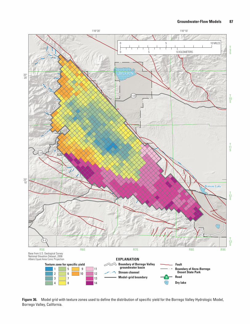
Groundwater-Flow Models 87
Figure 36. Model grid with texture zones used to define the distribution of specific yield for the Borrego Valley Hydrologic Model, Borrego Valley, California.
Clark Lake
BorregoSink
Benson Lake
T9S
T10S
T11S
T12S
T13S
R5E R6E R7E R8E R9EBase from U.S. Geological Survey National Elevation Dataset, 2006Albers Equal Area Conic Projection
S-22
S-22
S-2
78
116°10’116°20’
33°20’
33°10’
0
0 5 10
5 10 MILES
KILOMETERS
sac13-0509_Figure 36 Sy zones
EXPLANATIONTexture zone for specific yield
910
1234
5678
11121314
Model-grid boundaryStream channel
Boundary of Borrego Valley groundwater basin Boundary of Anza-Borrego
Desert State Park
Fault
Road78
Dry lake
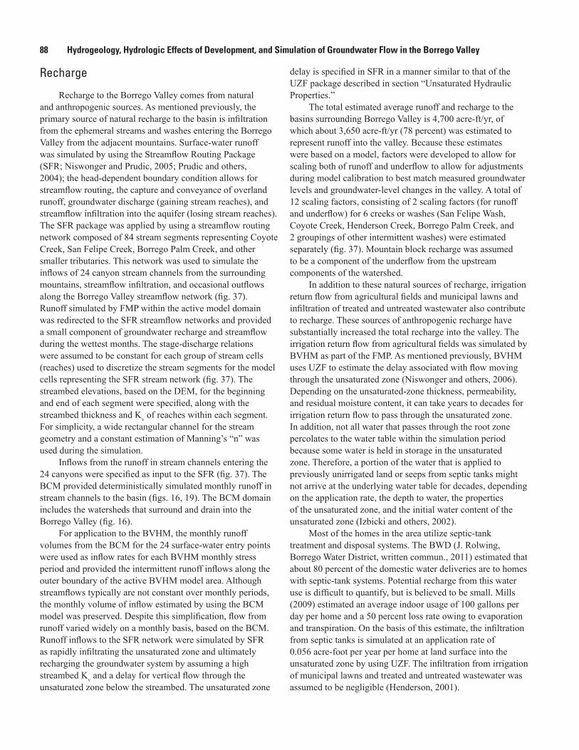
88 Hydrogeology, Hydrologic Effects of Development, and Simulation of Groundwater Flow in the Borrego Valley
Recharge
Recharge to the Borrego Valley comes from natural and anthropogenic sources. As mentioned previously, the primary source of natural recharge to the basin is infiltration from the ephemeral streams and washes entering the Borrego Valley from the adjacent mountains. Surface-water runoff was simulated by using the Streamflow Routing Package (SFR; Niswonger and Prudic, 2005; Prudic and others, 2004); the head-dependent boundary condition allows for streamflow routing, the capture and conveyance of overland runoff, groundwater discharge (gaining stream reaches), and streamflow infiltration into the aquifer (losing stream reaches). The SFR package was applied by using a streamflow routing network composed of 84 stream segments representing Coyote Creek, San Felipe Creek, Borrego Palm Creek, and other smaller tributaries. This network was used to simulate the inflows of 24 canyon stream channels from the surrounding mountains, streamflow infiltration, and occasional outflows along the Borrego Valley streamflow network (fig. 37). Runoff simulated by FMP within the active model domain was redirected to the SFR streamflow networks and provided a small component of groundwater recharge and streamflow during the wettest months. The stage-discharge relations were assumed to be constant for each group of stream cells (reaches) used to discretize the stream segments for the model cells representing the SFR stream network (fig. 37). The streambed elevations, based on the DEM, for the beginning and end of each segment were specified, along with the streambed thickness and Kv of reaches within each segment. For simplicity, a wide rectangular channel for the stream geometry and a constant estimation of Manning’s “n” was used during the simulation.
Inflows from the runoff in stream channels entering the 24 canyons were specified as input to the SFR (fig. 37). The BCM provided deterministically simulated monthly runoff in stream channels to the basin (figs. 16, 19). The BCM domain includes the watersheds that surround and drain into the Borrego Valley (fig. 16).
For application to the BVHM, the monthly runoff volumes from the BCM for the 24 surface-water entry points were used as inflow rates for each BVHM monthly stress period and provided the intermittent runoff inflows along the outer boundary of the active BVHM model area. Although streamflows typically are not constant over monthly periods, the monthly volume of inflow estimated by using the BCM model was preserved. Despite this simplification, flow from runoff varied widely on a monthly basis, based on the BCM. Runoff inflows to the SFR network were simulated by SFR as rapidly infiltrating the unsaturated zone and ultimately recharging the groundwater system by assuming a high streambed Kv and a delay for vertical flow through the unsaturated zone below the streambed. The unsaturated zone
delay is specified in SFR in a manner similar to that of the UZF package described in section “Unsaturated Hydraulic Properties.”
The total estimated average runoff and recharge to the basins surrounding Borrego Valley is 4,700 acre-ft/yr, of which about 3,650 acre-ft/yr (78 percent) was estimated to represent runoff into the valley. Because these estimates were based on a model, factors were developed to allow for scaling both of runoff and underflow to allow for adjustments during model calibration to best match measured groundwater levels and groundwater-level changes in the valley. A total of 12 scaling factors, consisting of 2 scaling factors (for runoff and underflow) for 6 creeks or washes (San Felipe Wash, Coyote Creek, Henderson Creek, Borrego Palm Creek, and 2 groupings of other intermittent washes) were estimated separately (fig. 37). Mountain block recharge was assumed to be a component of the underflow from the upstream components of the watershed.
In addition to these natural sources of recharge, irrigation return flow from agricultural fields and municipal lawns and infiltration of treated and untreated wastewater also contribute to recharge. These sources of anthropogenic recharge have substantially increased the total recharge into the valley. The irrigation return flow from agricultural fields was simulated by BVHM as part of the FMP. As mentioned previously, BVHM uses UZF to estimate the delay associated with flow moving through the unsaturated zone (Niswonger and others, 2006). Depending on the unsaturated-zone thickness, permeability, and residual moisture content, it can take years to decades for irrigation return flow to pass through the unsaturated zone. In addition, not all water that passes through the root zone percolates to the water table within the simulation period because some water is held in storage in the unsaturated zone. Therefore, a portion of the water that is applied to previously unirrigated land or seeps from septic tanks might not arrive at the underlying water table for decades, depending on the application rate, the depth to water, the properties of the unsaturated zone, and the initial water content of the unsaturated zone (Izbicki and others, 2002).
Most of the homes in the area utilize septic-tank treatment and disposal systems. The BWD (J. Rolwing, Borrego Water District, written commun., 2011) estimated that about 80 percent of the domestic water deliveries are to homes with septic-tank systems. Potential recharge from this water use is difficult to quantify, but is believed to be small. Mills (2009) estimated an average indoor usage of 100 gallons per day per home and a 50 percent loss rate owing to evaporation and transpiration. On the basis of this estimate, the infiltration from septic tanks is simulated at an application rate of 0.056 acre-foot per year per home at land surface into the unsaturated zone by using UZF. The infiltration from irrigation of municipal lawns and treated and untreated wastewater was assumed to be negligible (Henderson, 2001).
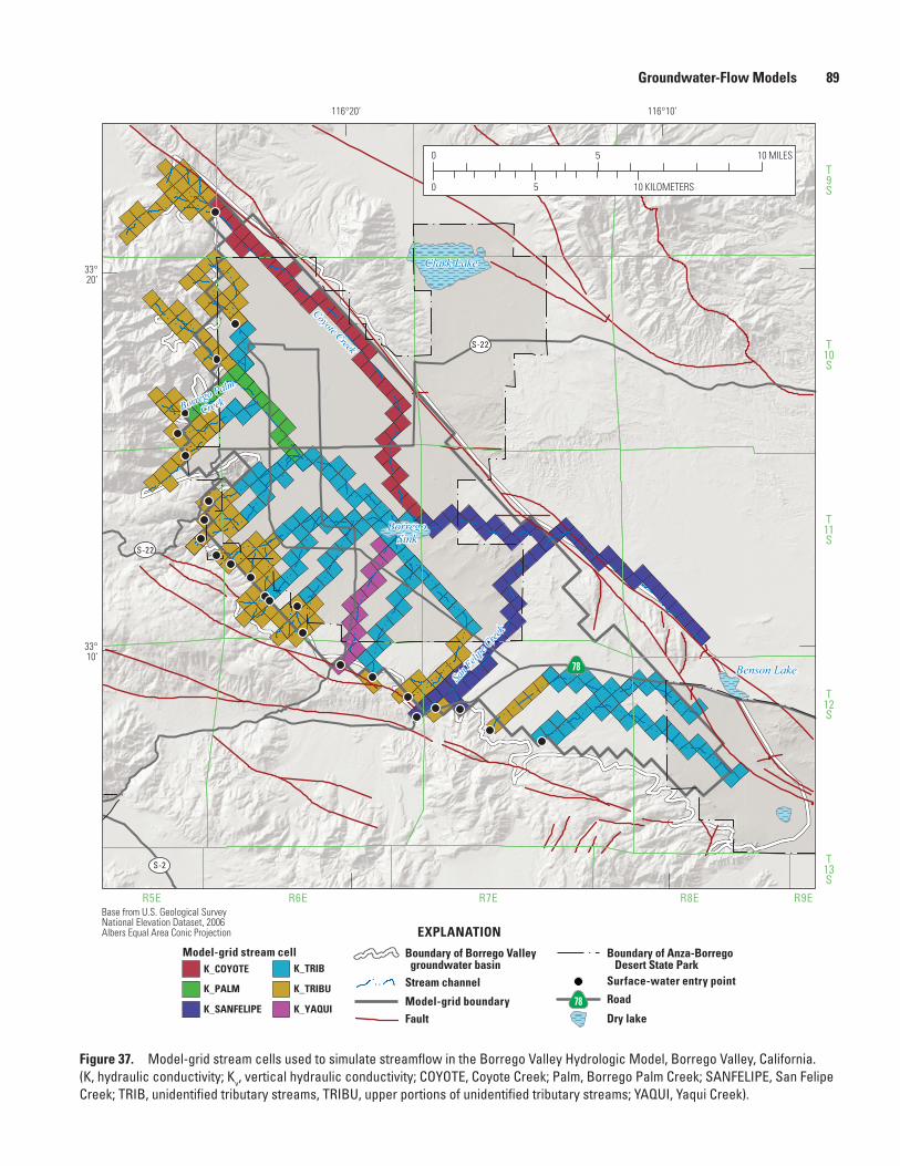
Groundwater-Flow Models 89
Figure 37. Model-grid stream cells used to simulate streamflow in the Borrego Valley Hydrologic Model, Borrego Valley, California. (K, hydraulic conductivity; Kv, vertical hydraulic conductivity; COYOTE, Coyote Creek; Palm, Borrego Palm Creek; SANFELIPE, San Felipe Creek; TRIB, unidentified tributary streams, TRIBU, upper portions of unidentified tributary streams; YAQUI, Yaqui Creek).
Clark Lake
BorregoSink
Benson Lake
T9S
T10S
T11S
T12S
T13S
R5E R6E R7E R8E R9EBase from U.S. Geological Survey National Elevation Dataset, 2006Albers Equal Area Conic Projection
S-22
S-22
S-2
78
116°10’116°20’
33°20’
33°10’
0
0 5 10
5 10 MILES
KILOMETERS
sac13-0509_Figure 37 Stream Grid
EXPLANATION
Coyote Creek
Borrego Palm
Creek
San F
elipe
Cree
k
Road78
Model-grid stream cellK_COYOTE
K_PALM
K_SANFELIPE
K_TRIB
K_TRIBU
K_YAQUI
Surface-water entry point
Model-grid boundary
Stream channel
Boundary of Borrego Valley groundwater basin
Boundary of Anza-Borrego Desert State Park
Fault Dry lake
90 Hydrogeology, Hydrologic Effects of Development, and Simulation of Groundwater Flow in the Borrego Valley
Water-Balance Subregions The evolution of the landscape is a combination of
changes in land use and related land ownership in Borrego Valley over the 66 years of the historical simulation, 1945–2010. Parcels defined for 2010 were used to define land ownership and divide the valley into WBSs (fig. 38). The footprint of these WBSs was held constant throughout the simulation; however, the land-use types change over time in each WBS and reflect the evolution of land use. The land-use type determines the water demand for native vegetation or irrigated crops, which is used to calculate the required groundwater pumping for irrigation.
Landscape Water UseThe FMP provides a coupled simulation of the
groundwater and surface-water components of the hydrologic cycle for irrigated and non-irrigated areas. A dynamic allocation of groundwater recharge and groundwater pumping was simulated on the basis of residual crop-water demand after surface-water deliveries (in Borrego Valley surface water is not used for irrigation) and root uptake from shallow groundwater. For a given stress period, the estimation of irrigation groundwater pumping in FMP was dependent on satisfying demands for ET from precipitation and variable irrigation efficiencies that govern the availability of excess water available for deep percolation. For a complete description of these components, please see the FMP manual (Schmid and others, 2006a). The FMP not only estimates supply, demand, movement, and consumption of irrigation water, but also estimates these components for natural vegetation. To summarize, the use and movement of water on the landscape is fully coupled with streamflow and groundwater flow and is dependent on atmospheric (and soil) conditions through precipitation and reference ET.
The FMP simulates the demand components representing the crop irrigation requirement (CIR) that are subject to crop and farm-specific irrigation efficiencies and the supply components representing precipitation, direct uptake from groundwater, uptake of soil moisture, and irrigation from groundwater pumping. The FMP also simulates additional head-dependent inflows and outflows from the landscape, such as surface runoff from precipitation and irrigation to the streamflow network and groundwater recharge as deep percolation of water in excess of actual evapotranspiration (ETact) and runoff (Schmid and others, 2006a, b; Schmid and Hanson, 2009). Changes in soil moisture were not simulated by the FMP and were assumed to be negligible at the monthly time scale.
Inflows and outflows throughout the WBSs on the landscape were simulated by FMP. Water mass within each WBS was calculated and balanced for each simulation time step (Schmid and others, 2006a, b; Schmid and Hanson, 2009). The FMP dynamically integrates irrigation water demand from ET with water supply and irrigation efficiencies. In order to do this, the FMP first calculates crop water demand as the transpiration or consumption of water by plants and the
related evaporation on the basis of cell-by-cell estimations for each WBS. The FMP then determines a residual plant water demand that cannot be satisfied by precipitation and by root uptake from groundwater, if available from shallow groundwater near the root zone. This residual water demand is the vegetation’s irrigation requirement for the cells with irrigated crops (that is, exclusive of any natural vegetation), which is called CIR and is calculated on a cell-by-cell basis.
The CIR is then adjusted (increased) by accounting for evaporative losses from irrigation and other inefficiency losses to yield a final total farm delivery requirement (TFDR). For Borrego Valley, where groundwater is the sole source of irrigation water, FMP attempts to satisfy the TFDR by using groundwater pumpage. This demand is not met when the demand exceeds the capacity of the wells for a specific WBS, either because groundwater levels dropped below the maximum screen-interval depth or the pumping rate of a given well is exceeded. The amount of excess water from irrigation (irrigation efficiencies) and precipitation that is not effectively used for crop growth then becomes either overland runoff to nearby streams or groundwater recharge as deep percolation below the root zone, on the basis of parameters specified in the FMP. In the BVHM, all the excess water ultimately becomes groundwater recharge. Thus, the FMP dynamically links the demand, supply, and related change in head. All of the supply and demand components are then tabulated into WBS budgets, which complement the groundwater flow, and streamflow budgets, which collectively represent the hydrologic cycle within Borrego Valley.
In order to estimate the inflows and outflows, the FMP dynamically simulates the supply and demand components for a WBS by integrating the following computational components specific to Borrego Valley’s hydrologic setting:1. TFDR, which is largely dependent on the CIR, but also
depends on efficiency, climate variability (PET and precipitation), and variable aquifer head.
2. Groundwater pumping, which is equivalent to the TFDR in the BVHM.
3. Net recharge (deep percolation) to groundwater, which is taken to be the sum of excess irrigation and precipitation minus ET from groundwater.
OWHM maintains a mass balance for each WBS budget, for the streamflow network, and for the groundwater-flow system. Flows between these budgets are accommodated by head-dependent inflows and outflows, such as ETact, runoff and infiltration, or ET from groundwater. For the BVHM, the processes of evaporation, transpiration, runoff, deep percolation to groundwater, and groundwater pumping were simulated. The simulated groundwater pumpage reflects climatic differences and differences in agricultural practices (including irrigation method) among defined WBSs. The BVHM model provides a detailed transient analysis of changes in groundwater storage in relation to climatic variability, urbanization, land use, and changes in irrigated agriculture.
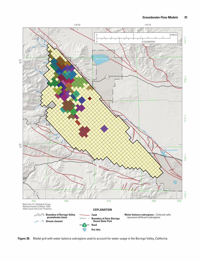
Groundwater-Flow Models 91
Figure 38. Model grid with water balance subregions used to account for water usage in the Borrego Valley, California.
Clark Lake
BorregoSink
Benson Lake
T9S
T10S
T11S
T12S
T13S
R5E R6E R7E R8E R9EBase from U.S. Geological Survey National Elevation Dataset, 2006Albers Equal Area Conic Projection
S-22
S-22
S-2
78
116°10’116°20’
33°20’
33°10’
0
0 5 10
5 10 MILES
KILOMETERS
sac13-0509_Figure 38 water balance regions
EXPLANATION
Water balance subregions—Colored cells represent different subregions
Stream channel
Boundary of Borrego Valley groundwater basin Boundary of Anza-Borrego
Desert State Park
Fault
Road78
Dry lake
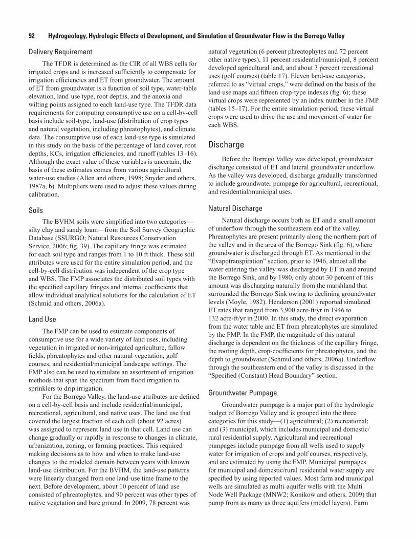
92 Hydrogeology, Hydrologic Effects of Development, and Simulation of Groundwater Flow in the Borrego Valley
Delivery RequirementThe TFDR is determined as the CIR of all WBS cells for
irrigated crops and is increased sufficiently to compensate for irrigation efficiencies and ET from groundwater. The amount of ET from groundwater is a function of soil type, water-table elevation, land-use type, root depths, and the anoxia and wilting points assigned to each land-use type. The TFDR data requirements for computing consumptive use on a cell-by-cell basis include soil-type, land-use (distribution of crop types and natural vegetation, including phreatophytes), and climate data. The consumptive use of each land-use type is simulated in this study on the basis of the percentage of land cover, root depths, KCs, irrigation efficiencies, and runoff (tables 13–16). Although the exact value of these variables is uncertain, the basis of these estimates comes from various agricultural water-use studies (Allen and others, 1998; Snyder and others, 1987a, b). Multipliers were used to adjust these values during calibration.
SoilsThe BVHM soils were simplified into two categories—
silty clay and sandy loam—from the Soil Survey Geographic Database (SSURGO; Natural Resources Conservation Service, 2006; fig. 39). The capillary fringe was estimated for each soil type and ranges from 1 to 10 ft thick. These soil attributes were used for the entire simulation period, and the cell-by-cell distribution was independent of the crop type and WBS. The FMP associates the distributed soil types with the specified capillary fringes and internal coefficients that allow individual analytical solutions for the calculation of ET (Schmid and others, 2006a).
Land UseThe FMP can be used to estimate components of
consumptive use for a wide variety of land uses, including vegetation in irrigated or non-irrigated agriculture, fallow fields, phreatophytes and other natural vegetation, golf courses, and residential/municipal landscape settings. The FMP also can be used to simulate an assortment of irrigation methods that span the spectrum from flood irrigation to sprinklers to drip irrigation.
For the Borrego Valley, the land-use attributes are defined on a cell-by-cell basis and include residential/municipal, recreational, agricultural, and native uses. The land use that covered the largest fraction of each cell (about 92 acres) was assigned to represent land use in that cell. Land use can change gradually or rapidly in response to changes in climate, urbanization, zoning, or farming practices. This required making decisions as to how and when to make land-use changes to the modeled domain between years with known land-use distribution. For the BVHM, the land-use patterns were linearly changed from one land-use time frame to the next. Before development, about 10 percent of land use consisted of phreatophytes, and 90 percent was other types of native vegetation and bare ground. In 2009, 78 percent was
natural vegetation (6 percent phreatophytes and 72 percent other native types), 11 percent residential/municipal, 8 percent developed agricultural land, and about 3 percent recreational uses (golf courses) (table 17). Eleven land-use categories, referred to as “virtual crops,” were defined on the basis of the land-use maps and fifteen crop-type indexes (fig. 6); these virtual crops were represented by an index number in the FMP (tables 15–17). For the entire simulation period, these virtual crops were used to drive the use and movement of water for each WBS.
DischargeBefore the Borrego Valley was developed, groundwater
discharge consisted of ET and lateral groundwater underflow. As the valley was developed, discharge gradually transformed to include groundwater pumpage for agricultural, recreational, and residential/municipal uses.
Natural DischargeNatural discharge occurs both as ET and a small amount
of underflow through the southeastern end of the valley. Phreatophytes are present primarily along the northern part of the valley and in the area of the Borrego Sink (fig. 6), where groundwater is discharged through ET. As mentioned in the “Evapotranspiration” section, prior to 1946, almost all the water entering the valley was discharged by ET in and around the Borrego Sink, and by 1980, only about 30 percent of this amount was discharging naturally from the marshland that surrounded the Borrego Sink owing to declining groundwater levels (Moyle, 1982). Henderson (2001) reported simulated ET rates that ranged from 3,900 acre-ft/yr in 1946 to 132 acre-ft/yr in 2000. In this study, the direct evaporation from the water table and ET from phreatophytes are simulated by the FMP. In the FMP, the magnitude of this natural discharge is dependent on the thickness of the capillary fringe, the rooting depth, crop-coefficients for phreatophytes, and the depth to groundwater (Schmid and others, 2006a). Underflow through the southeastern end of the valley is discussed in the “Specified (Constant) Head Boundary” section.
Groundwater PumpageGroundwater pumpage is a major part of the hydrologic
budget of Borrego Valley and is grouped into the three categories for this study—(1) agricultural; (2) recreational; and (3) municipal, which includes municipal and domestic/rural residential supply. Agricultural and recreational pumpages include pumpage from all wells used to supply water for irrigation of crops and golf courses, respectively, and are estimated by using the FMP. Municipal pumpages for municipal and domestic/rural residential water supply are specified by using reported values. Most farm and municipal wells are simulated as multi-aquifer wells with the Multi-Node Well Package (MNW2; Konikow and others, 2009) that pump from as many as three aquifers (model layers). Farm
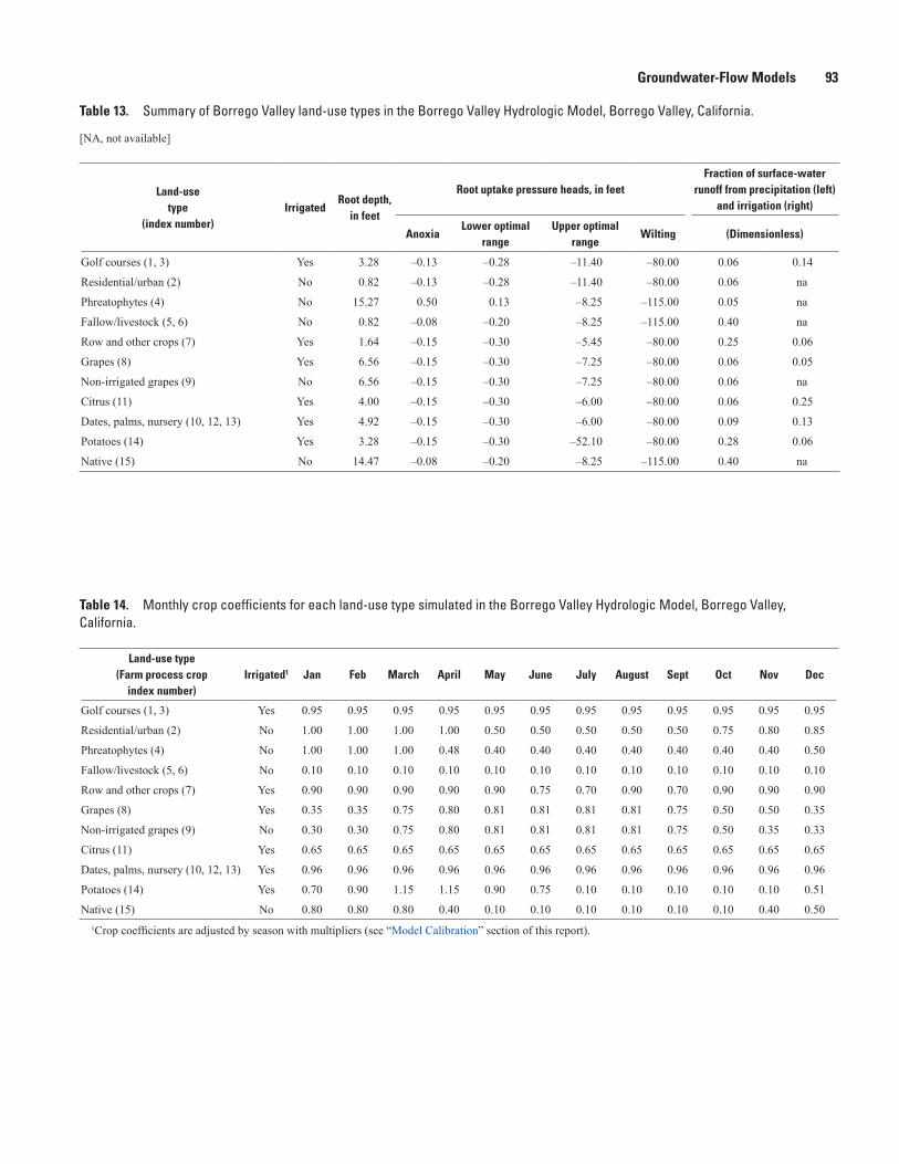
Groundwater-Flow Models 93
Table 13. Summary of Borrego Valley land-use types in the Borrego Valley Hydrologic Model, Borrego Valley, California.
[NA, not available]
Land-use type
(index number)Irrigated
Root depth, in feet
Root uptake pressure heads, in feetFraction of surface-water
runoff from precipitation (left) and irrigation (right)
AnoxiaLower optimal
rangeUpper optimal
rangeWilting (Dimensionless)
Golf courses (1, 3) Yes 3.28 –0.13 –0.28 –11.40 –80.00 0.06 0.14
Residential/urban (2) No 0.82 –0.13 –0.28 –11.40 –80.00 0.06 na
Phreatophytes (4) No 15.27 0.50 0.13 –8.25 –115.00 0.05 na
Fallow/livestock (5, 6) No 0.82 –0.08 –0.20 –8.25 –115.00 0.40 na
Row and other crops (7) Yes 1.64 –0.15 –0.30 –5.45 –80.00 0.25 0.06
Grapes (8) Yes 6.56 –0.15 –0.30 –7.25 –80.00 0.06 0.05
Non-irrigated grapes (9) No 6.56 –0.15 –0.30 –7.25 –80.00 0.06 na
Citrus (11) Yes 4.00 –0.15 –0.30 –6.00 –80.00 0.06 0.25
Dates, palms, nursery (10, 12, 13) Yes 4.92 –0.15 –0.30 –6.00 –80.00 0.09 0.13
Potatoes (14) Yes 3.28 –0.15 –0.30 –52.10 –80.00 0.28 0.06
Native (15) No 14.47 –0.08 –0.20 –8.25 –115.00 0.40 na
Table 14. Monthly crop coefficients for each land-use type simulated in the Borrego Valley Hydrologic Model, Borrego Valley, California.
Land-use type (Farm process crop
index number)Irrigated1 Jan Feb March April May June July August Sept Oct Nov Dec
Golf courses (1, 3) Yes 0.95 0.95 0.95 0.95 0.95 0.95 0.95 0.95 0.95 0.95 0.95 0.95
Residential/urban (2) No 1.00 1.00 1.00 1.00 0.50 0.50 0.50 0.50 0.50 0.75 0.80 0.85
Phreatophytes (4) No 1.00 1.00 1.00 0.48 0.40 0.40 0.40 0.40 0.40 0.40 0.40 0.50
Fallow/livestock (5, 6) No 0.10 0.10 0.10 0.10 0.10 0.10 0.10 0.10 0.10 0.10 0.10 0.10
Row and other crops (7) Yes 0.90 0.90 0.90 0.90 0.90 0.75 0.70 0.90 0.70 0.90 0.90 0.90
Grapes (8) Yes 0.35 0.35 0.75 0.80 0.81 0.81 0.81 0.81 0.75 0.50 0.50 0.35
Non-irrigated grapes (9) No 0.30 0.30 0.75 0.80 0.81 0.81 0.81 0.81 0.75 0.50 0.35 0.33
Citrus (11) Yes 0.65 0.65 0.65 0.65 0.65 0.65 0.65 0.65 0.65 0.65 0.65 0.65
Dates, palms, nursery (10, 12, 13) Yes 0.96 0.96 0.96 0.96 0.96 0.96 0.96 0.96 0.96 0.96 0.96 0.96
Potatoes (14) Yes 0.70 0.90 1.15 1.15 0.90 0.75 0.10 0.10 0.10 0.10 0.10 0.51
Native (15) No 0.80 0.80 0.80 0.40 0.10 0.10 0.10 0.10 0.10 0.10 0.40 0.501Crop coefficients are adjusted by season with multipliers (see “Model Calibration” section of this report).
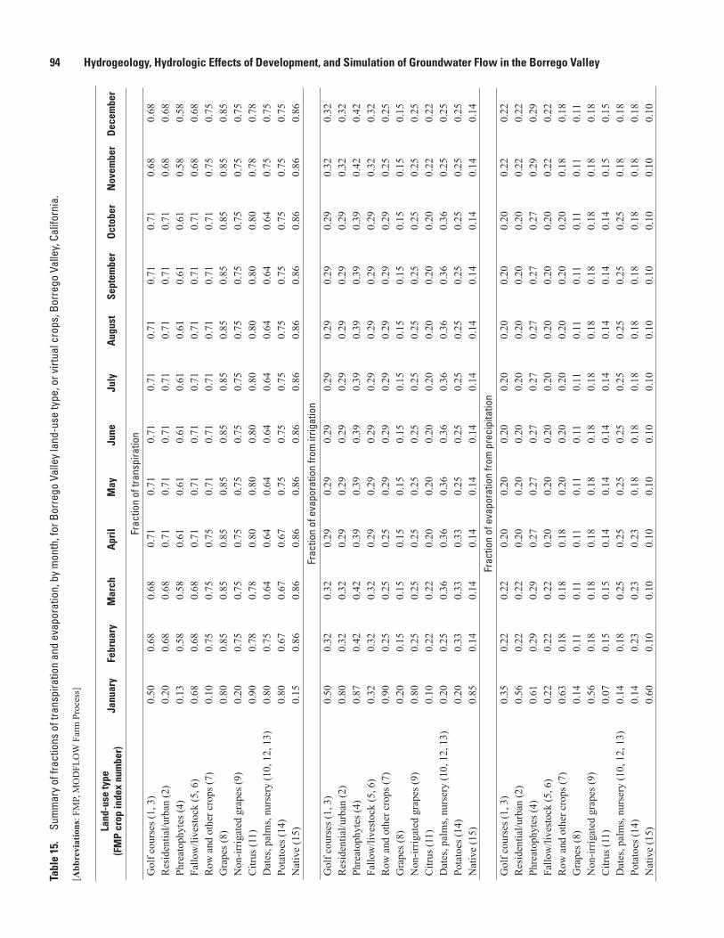
94 Hydrogeology, Hydrologic Effects of Development, and Simulation of Groundwater Flow in the Borrego ValleyTa
ble
15.
Sum
mar
y of
frac
tions
of t
rans
pira
tion
and
evap
orat
ion,
by
mon
th, f
or B
orre
go V
alle
y la
nd-u
se ty
pe, o
r virt
ual c
rops
, Bor
rego
Val
ley,
Cal
iforn
ia.
[Abb
revi
atio
ns: F
MP,
MO
DFL
OW
Far
m P
roce
ss]
Land
-use
type
(FM
P cr
op in
dex
num
ber)
Janu
ary
Febr
uary
Mar
chA
pril
May
June
July
Aug
ust
Sept
embe
rO
ctob
erN
ovem
ber
Dec
embe
r
Frac
tion
of tr
ansp
iratio
nG
olf c
ours
es (1
, 3)
0.50
0.68
0.68
0.71
0.71
0.71
0.71
0.71
0.71
0.71
0.68
0.68
Res
iden
tial/u
rban
(2)
0.20
0.68
0.68
0.71
0.71
0.71
0.71
0.71
0.71
0.71
0.68
0.68
Phre
atop
hyte
s (4)
0.13
0.58
0.58
0.61
0.61
0.61
0.61
0.61
0.61
0.61
0.58
0.58
Fallo
w/li
vest
ock
(5, 6
)0.
680.
680.
680.
710.
710.
710.
710.
710.
710.
710.
680.
68R
ow a
nd o
ther
cro
ps (7
)0.
100.
750.
750.
750.
710.
710.
710.
710.
710.
710.
750.
75G
rape
s (8)
0.80
0.85
0.85
0.85
0.85
0.85
0.85
0.85
0.85
0.85
0.85
0.85
Non
-irrig
ated
gra
pes (
9)0.
200.
750.
750.
750.
750.
750.
750.
750.
750.
750.
750.
75C
itrus
(11)
0.90
0.78
0.78
0.80
0.80
0.80
0.80
0.80
0.80
0.80
0.78
0.78
Dat
es, p
alm
s, nu
rser
y (1
0, 1
2, 1
3)0.
800.
750.
640.
640.
640.
640.
640.
640.
640.
640.
750.
75Po
tato
es (1
4)0.
800.
670.
670.
670.
750.
750.
750.
750.
750.
750.
750.
75N
ativ
e (1
5)0.
150.
860.
860.
860.
860.
860.
860.
860.
860.
860.
860.
86Fr
actio
n of
eva
pora
tion
from
irrig
atio
nG
olf c
ours
es (1
, 3)
0.50
0.32
0.32
0.29
0.29
0.29
0.29
0.29
0.29
0.29
0.32
0.32
Res
iden
tial/u
rban
(2)
0.80
0.32
0.32
0.29
0.29
0.29
0.29
0.29
0.29
0.29
0.32
0.32
Phre
atop
hyte
s (4)
0.87
0.42
0.42
0.39
0.39
0.39
0.39
0.39
0.39
0.39
0.42
0.42
Fallo
w/li
vest
ock
(5, 6
)0.
320.
320.
320.
290.
290.
290.
290.
290.
290.
290.
320.
32R
ow a
nd o
ther
cro
ps (7
)0.
900.
250.
250.
250.
290.
290.
290.
290.
290.
290.
250.
25G
rape
s (8)
0.20
0.15
0.15
0.15
0.15
0.15
0.15
0.15
0.15
0.15
0.15
0.15
Non
-irrig
ated
gra
pes (
9)0.
800.
250.
250.
250.
250.
250.
250.
250.
250.
250.
250.
25C
itrus
(11)
0.10
0.22
0.22
0.20
0.20
0.20
0.20
0.20
0.20
0.20
0.22
0.22
Dat
es, p
alm
s, nu
rser
y (1
0, 1
2, 1
3)0.
200.
250.
360.
360.
360.
360.
360.
360.
360.
360.
250.
25Po
tato
es (1
4)0.
200.
330.
330.
330.
250.
250.
250.
250.
250.
250.
250.
25N
ativ
e (1
5)0.
850.
140.
140.
140.
140.
140.
140.
140.
140.
140.
140.
14Fr
actio
n of
eva
pora
tion
from
pre
cipi
tatio
nG
olf c
ours
es (1
, 3)
0.35
0.22
0.22
0.20
0.20
0.20
0.20
0.20
0.20
0.20
0.22
0.22
Res
iden
tial/u
rban
(2)
0.56
0.22
0.22
0.20
0.20
0.20
0.20
0.20
0.20
0.20
0.22
0.22
Phre
atop
hyte
s (4)
0.61
0.29
0.29
0.27
0.27
0.27
0.27
0.27
0.27
0.27
0.29
0.29
Fallo
w/li
vest
ock
(5, 6
)0.
220.
220.
220.
200.
200.
200.
200.
200.
200.
200.
220.
22R
ow a
nd o
ther
cro
ps (7
)0.
630.
180.
180.
180.
200.
200.
200.
200.
200.
200.
180.
18G
rape
s (8)
0.14
0.11
0.11
0.11
0.11
0.11
0.11
0.11
0.11
0.11
0.11
0.11
Non
-irrig
ated
gra
pes (
9)0.
560.
180.
180.
180.
180.
180.
180.
180.
180.
180.
180.
18C
itrus
(11)
0.07
0.15
0.15
0.14
0.14
0.14
0.14
0.14
0.14
0.14
0.15
0.15
Dat
es, p
alm
s, nu
rser
y (1
0, 1
2, 1
3)0.
140.
180.
250.
250.
250.
250.
250.
250.
250.
250.
180.
18Po
tato
es (1
4)0.
140.
230.
230.
230.
180.
180.
180.
180.
180.
180.
180.
18N
ativ
e (1
5)0.
600.
100.
100.
100.
100.
100.
100.
100.
100.
100.
100.
10
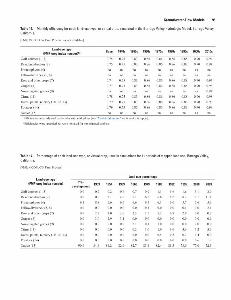
Groundwater-Flow Models 95
Table 16. Monthly efficiency for each land-use type, or virtual crop, simulated in the Borrego Valley Hydrologic Model, Borrego Valley, California.
[FMP, MODFLOW Farm Process; na, not available]
Land-use type(FMP crop index number)1,2 Base 1940s 1950s 1960s 1970s 1980s 1990s 2000s 2010s
Golf courses (1, 3) 0.75 0.75 0.83 0.86 0.86 0.86 0.88 0.90 0.94Residential/urban (2) 0.75 0.75 0.83 0.86 0.86 0.86 0.88 0.90 0.94Phreatophytes (4) na na na na na na na na naFallow/livestock (5, 6) na na na na na na na na naRow and other crops (7) 0.74 0.75 0.83 0.86 0.86 0.86 0.88 0.90 0.93Grapes (8) 0.77 0.75 0.83 0.86 0.86 0.86 0.88 0.90 0.96Non-irrigated grapes (9) na na na na na na na na 0.94Citrus (11) 0.78 0.75 0.83 0.86 0.86 0.86 0.88 0.90 0.98Dates, palms, nursery (10, 12, 13) 0.79 0.75 0.83 0.86 0.86 0.86 0.88 0.90 0.99Potatoes (14) 0.79 0.75 0.83 0.86 0.86 0.86 0.88 0.90 0.99Native (15) na na na na na na na na na
1Efficiencies were adjusted by decades with multipliers (see “Model Calibration” section of this report). 2Efficiencies were specified but were not used for nonirrigated land use.
Table 17. Percentage of each land-use type, or virtual crop, used in simulations for 11 periods of mapped land use, Borrego Valley, California.
[FMP, MODFLOW Farm Process]
Land-use type (FMP crop index number)
Land use percentage
Pre- development
1953 1954 1959 1968 1979 1980 1992 1995 2000 2009
Golf courses (1, 3) 0.0 0.2 0.2 0.4 0.7 0.9 1.1 1.6 1.6 3.1 3.0Residential/urban (2) 0.0 0.6 3.1 4.0 5.1 6.5 6.6 8.2 8.2 10.1 11.1Phreatophytes (4) 9.1 8.8 6.6 6.6 6.6 6.5 6.1 6.0 5.7 5.6 5.6Fallow/livestock (5, 6) 0.0 0.0 0.0 0.0 0.0 0.1 0.0 0.0 0.1 0.0 2.1Row and other crops (7) 0.0 2.7 3.0 3.0 2.5 1.5 1.2 0.7 2.0 0.0 0.0Grapes (8) 0.0 3.0 2.9 3.1 0.0 0.0 0.0 0.0 0.0 0.0 0.0Non-irrigated grapes (9) 0.0 0.0 0.0 0.0 2.1 0.1 1.0 0.0 0.0 0.0 0.0Citrus (11) 0.0 0.0 0.0 0.0 0.2 1.0 1.0 1.6 3.6 3.2 3.6Dates, palms, nursery (10, 12, 13) 0.0 0.0 0.0 0.0 0.0 0.0 0.5 0.5 0.7 0.4 0.9Potatoes (14) 0.0 0.0 0.0 0.0 0.0 0.0 0.0 0.0 0.0 0.6 1.2Native (15) 90.9 84.6 84.2 82.9 82.7 83.4 82.4 81.3 78.0 77.0 72.5
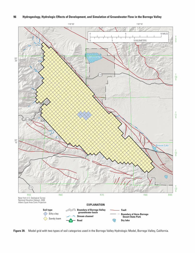
96 Hydrogeology, Hydrologic Effects of Development, and Simulation of Groundwater Flow in the Borrego Valley
Clark Lake
BorregoSink
Benson Lake
T9S
T10S
T11S
T12S
T13S
R5E R6E R7E R8E R9EBase from U.S. Geological Survey National Elevation Dataset, 2006Albers Equal Area Conic Projection
S-22
S-22
S-2
78
116°10’116°20’
33°20’
33°10’
0
0 5 10
5 10 MILES
KILOMETERS
sac13-0509_Figure 39 soils
EXPLANATION
Silty claySoil type
Sandy loamStream channel
Boundary of Borrego Valley groundwater basin
Road78
Boundary of Anza-Borrego Desert State Park
Fault
Dry lake
Figure 39. Model grid with two types of soil categories used in the Borrego Valley Hydrologic Model, Borrego Valley, California.
Groundwater-Flow Models 97
wells were simulated as a combination of single-aquifer farm wells (Schmid and others, 2006a) and multi-aquifer wells that collectively supply groundwater to each WBS (fig. 38), as needed, for irrigation during each monthly stress period. Pumpage from single-aquifer farm wells was simulated in the manner of the WEL package (Harbaugh and others, 2000), while the multi-aquifer wells were simulated with MNW2. Total pumpage for each WBS (virtual farm) was distributed among each of the farm wells within the WBS on the basis of the average pumping rate up to the pumping capacity of each well (which did not come into effect in this simulation) (Schmid and others, 2006a).
Agricultural Pumpage
Discharge from agricultural wells generally is not metered in the Borrego Valley. Therefore, agricultural water use is simulated by an indirect estimation of pumpage. The two most common methods of indirectly estimating agricultural pumpage utilize power consumption and consumptive use of water. The use of electric power records is considered unreliable for estimating pumpage because many wells are powered by either electric or diesel power sources, and there is the inherent complexity of additional uses for electricity on a farm-by-farm basis. Consumptive-use estimates, such as satellite remote-sensing derived estimates, are also considered unreliable because they do not account for the combined consumption of precipitation and water applied for irrigation and do not capture the variability in consumption with changing climate (Hanson and others, 2014; Schmid and others, 2006a). The estimation of agricultural pumpage by using the FMP provides physically based, dynamic, and linked pumpage estimates as an alternative to indirect methods (Schmid and others, 2006a).
Pumpage for agricultural supply is estimated as a combination of CIR and efficiencies required to satisfy the TFDR for all wells that deliver water to a particular WBS. Efficiencies include those from irrigation-water conveyance (canals or irrigation pipes) and potential losses from runoff and deep percolation below the root zone during irrigation. The groundwater pumpage required to satisfy TFDR can be estimated by taking into account any potential surface-water supply, the efficiency of irrigation (fractions of losses to runoff and deep percolation), effective precipitation, ET from groundwater, and fractions of transpiration and evaporation within each model cell. Because all irrigation is supplied by groundwater pumpage in Borrego Valley, no surface-water supplies were simulated. Unmetered pumpage is estimated by the FMP on the basis the TFDR. As many as 71 farm wells were used to simulate pumpage for irrigation; the number of wells, and the pumpage, vary over time. There is no known reported pumpage for Borrego Valley that can be used as additional calibration data for agricultural pumpage.
For each well, the aquifer for which pumpage was simulated was based on the available construction information. Specifically, the drillers’ logs were analyzed, and the top
and bottom intervals for each well were assigned. The FMP allocated pumpage to wells within a WBS by the average fraction of total required pumpage, up to the capacity specified on the drillers’ logs for each well. Figure 40 shows the distribution of simulated annual pumpage by aquifer.
Recreational Pumpage
Recreational water use, which is predominantly irrigation of golf courses, is also simulated by the FMP. As mentioned previously, the BWD supplies groundwater to the Rams Hill golf course and development. Therefore, this pumpage was subtracted from the total reported municipal pumpage values used in the model. The reported amount of water used by Rams Hill was used as a calibration target to constrain the FMP-derived pumpage estimate for this water use.
Municipal Pumpage
Pumpage for municipal and domestic/rural residential water supply was based on selected reported monthly and annual pumpage on a well-by-well basis for the ID and BSPCSD wells (see “Municipal Water Use” section). The actual locations of municipal-supply wells were used in the model, and the locations of domestic wells were either actual or virtual in selected land parcels that were represented by WBSs (figs. 9, 38). MNW2 was used to simulate municipal groundwater pumpage. The open-screened interval or total depth was used to identify the model layers from which pumping occurred.
Groundwater Inflows and OutflowsBoundary conditions were applied at some model cells
to simulate the inflows and outflows from the active model region as groundwater underflow and intermittent stream inflows (fig. 37). Three general types of boundary conditions were used in the model: specified flow, specified head, and head-dependent flow boundaries. The head-dependent flow boundaries were only used for stream infiltration and underflow in stream channels and are not discussed in this section. Inflows and outflows simulated as flows across the hydrologic boundaries include recharge and discharge for the groundwater system, as well as interdependent flows, such as ET and irrigation, between groundwater, streams, and the landscape.
Specified (No Flow) Flow BoundariesNo-flow boundaries were used for the bottom of the
model and most lateral boundaries. The lower boundary was defined by the estimate of the depth of the basement rock. Lateral no-flow boundaries represented the contact between the low-permeability crystalline rocks that bound the foothills and the unconsolidated alluvial sediments of Borrego Valley (figs. 7, 34). Lateral boundaries on the east were coincident with the northwest-southeast trending Coyote Creek fault.
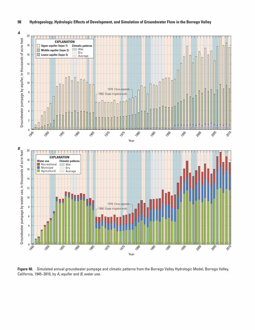
98 Hydrogeology, Hydrologic Effects of Development, and Simulation of Groundwater Flow in the Borrego Valley
sac13-0509_fig40_updated
Figure 40 pumpage by layer
A
B
0
2
4
6
8
10
12
18
16
14
20
1945
1950
1955
1960
1965
1970
1975
1980
1985
1990
1995
2000
2005
2010
Grou
ndw
ater
pum
page
by
aqui
fer,
in th
ousa
nds
of a
cre-
feet
Year
1945
1950
1955
1960
1965
1970
1975
1980
1985
1990
1995
2000
2005
2010
Year
0
2
4
6
8
10
12
18
16
14
20
Grou
ndw
ater
pum
page
by
wat
er u
se, i
n th
ousa
nds
of a
cre-
feet
EXPLANATIONUpper aquifer (layer 1)
Middle aquifer (layer 2)
Lower aquifer (layer 3)
EXPLANATION
Recreational
Agricultural
Climatic patternsWater useWetDryAverage
Climatic patternsWetDryAverage
Municipal
1966: Grape irrigation ends
1978: Citrus expands
1966: Grape irrigation ends
1978: Citrus expands
Figure 40. Simulated annual groundwater pumpage and climatic patterns from the Borrego Valley Hydrologic Model, Borrego Valley, California, 1945–2010, by A, aquifer and B, water use.
Groundwater-Flow Models 99
Specified Flow BoundariesGroundwater underflow was simulated by using the
Flow Head Boundary (FHB1) Package (Leake and Lilly, 1997); this head-dependent boundary condition allowed for underflow from the upstream portions of the watershed. The FHB1 package was applied by using 24 areas of alluvium along stream segments representing Coyote Creek, San Felipe Creek, Borrego Palm Creek, and other smaller tributaries. The underflow for each of the 24 canyons was spread among the cells at the edge of the model domain in these canyons. As in the SFR, the BCM provides deterministically simulated monthly estimates of the underflow from the adjacent mountains and basins (figs. 16, 19). The rate of underflow was simplified as an average for the simulation period to allow for the time integration of variable travel times of saturated and unsaturated groundwater-flow processes in the upstream portions of the watershed. As mentioned previously, scaling factors for six creeks or washes (San Felipe Wash, Coyote Creek, Henderson Creek, Borrego Palm Creek, and two groupings of other intermittent washes) were estimated separately (fig. 37). Mountain block recharge was assumed to be a component of the underflow from the upstream components of the watershed.
Specified (Constant) Head BoundaryThe farthest downstream region of the Borrego Valley
is a lateral hydrologic boundary of the groundwater-flow system that was simulated as a head-dependent flow boundary (fig. 34). This region represents a hydraulic connection with the valley to the southeast. It was simulated by using the Constant Head Boundary Package (CHD; Harbaugh, 2005). Constant-head cells were placed near lower Borrego Valley in the vicinity of Ocotillo Wells (fig. 33) because groundwater levels in that area (approximately mean sea level) indicate a steady-state condition (Mitten and others, 1988). Constant-head boundaries were specified in three cells in layer 3 with time-constant boundary heads. On the basis of data from Ocotillo Wells and previous simulations, this area of Borrego Valley does not appear to be affected by groundwater-level fluctuations or variations in groundwater discharge and recharge in the upper part of the aquifer system and can be treated as a constant-head boundary (Mitten and others, 1988).
Model Calibration
Calibration of the BVHM was accomplished by using a combination of trial-and-error and automated processes to determine the set of parameter values that minimized misfits (residuals) between observed (calibration-targets: heads and flows) and simulated values. The hydrologic framework and consumptive-use properties were modified as part of this process. The BVHM requires specification of about 100 parameters that vary spatially and temporally, making it a challenge to optimize parameter estimation. As a result, parameterization was introduced to allow a limited number of parameter values to define the model inputs that still vary in space and time.
Parameter DataHydraulic properties were estimated by using the Gauss-
Marquardt-Levenberg method, a widely used algorithm employed in PEST (Doherty, 2010a). This method modifies the initial values of parameters supplied by the modeler and subsequently adjusts these values such that the weighted sum of the squared differences between the observations and their corresponding model-simulated values is minimized. Each model cell is populated with values for each physical property (for example, K or specific yield). For most hydrologic models, this can result in an extremely large number of parameters, which can be reduced by using parameterization techniques such as zonation (for example, Doherty, 2003; Doherty and others, 2010a). In the BVHM presented in this report, there are many sources of nonlinearity, and the parameter-estimation problem has a relatively large number of parameters (highly parameterized) because many physical processes are being simulated.
Following Hill and Tiedeman (2007), the term “parameter” is used to define model inputs. Because the BVHM includes many complex hydrologic processes requiring that parameters be distributed in space and time, the potential number of model parameters that could be estimated is large. Therefore, model parameterization and the approach to parameter estimation were designed to estimate a limited number of parameter values that sufficiently define the simulated processes. The parameter values were adjusted by a combination of informed estimates (for example, professional judgement, expected values gleaned from the literature) and a systematic application of the parameter estimation method in order to narrow the range of possible solutions to produce simulated values that best matched the measured observations. Many of the parameters were specified apriori, and 137 parameters (table 18) were estimated during the automated calibration process. Fewer parameters often were estimated simultaneously for single, preliminary calibration runs. Extensive parameterization was used to characterize the following properties:
• Hydraulic conductivities, such as aquifer Kh and Kv in model layers 1–3, including an estimation of the power mean (described later), Kv of the streambed, the height of the capillary fringe, and the saturated Kv used in the computation of unsaturated Kvs of the unsaturated zone.
• Storage properties, such as specific yield of model layers 1–3 (where appropriate), specific storage of model layers 1–3, and saturated water content and initial water content of the unsaturated zone for the streambeds and, generally, for the rest of the valley.
• Scalar multipliers for runoff and underflow from the upstream portions of the watershed.
• Parameters within the landscape, such as scalar multipliers over time for irrigation efficiencies, stress factors for crop coefficients, and fractions of runoff both from precipitation and irrigation.
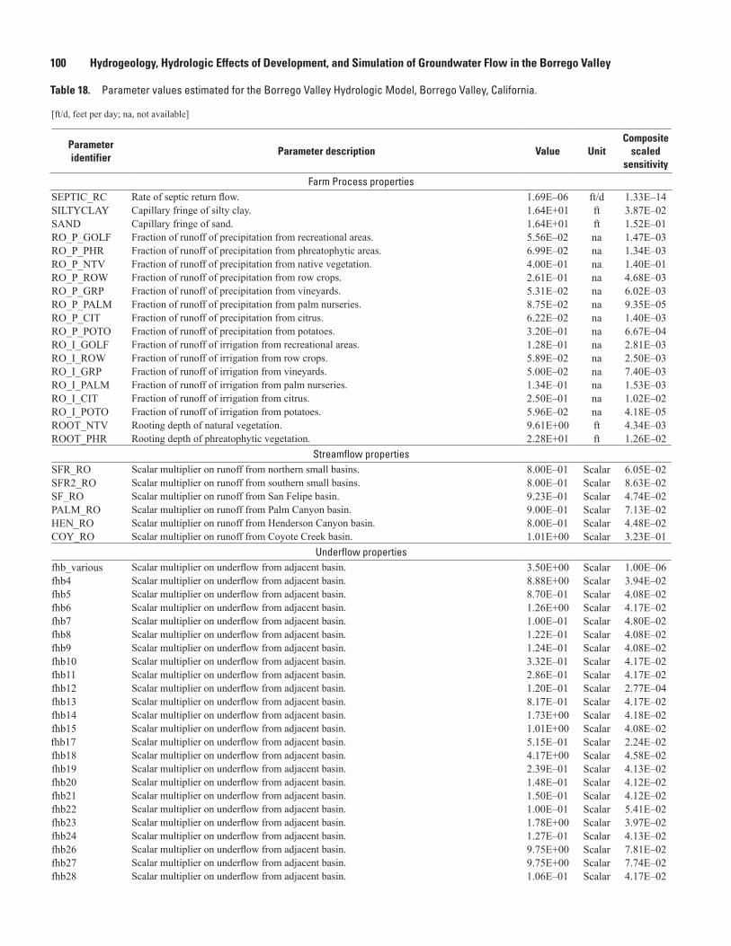
100 Hydrogeology, Hydrologic Effects of Development, and Simulation of Groundwater Flow in the Borrego Valley
Table 18. Parameter values estimated for the Borrego Valley Hydrologic Model, Borrego Valley, California.—Continued
[ft/d, feet per day; na, not available]
Parameter identifier
Parameter description Value UnitComposite
scaled sensitivity
Farm Process propertiesSEPTIC_RC Rate of septic return flow. 1.69E–06 ft/d 1.33E–14SILTYCLAY Capillary fringe of silty clay. 1.64E+01 ft 3.87E–02SAND Capillary fringe of sand. 1.64E+01 ft 1.52E–01RO_P_GOLF Fraction of runoff of precipitation from recreational areas. 5.56E–02 na 1.47E–03RO_P_PHR Fraction of runoff of precipitation from phreatophytic areas. 6.99E–02 na 1.34E–03RO_P_NTV Fraction of runoff of precipitation from native vegetation. 4.00E–01 na 1.40E–01RO_P_ROW Fraction of runoff of precipitation from row crops. 2.61E–01 na 4.68E–03RO_P_GRP Fraction of runoff of precipitation from vineyards. 5.31E–02 na 6.02E–03RO_P_PALM Fraction of runoff of precipitation from palm nurseries. 8.75E–02 na 9.35E–05RO_P_CIT Fraction of runoff of precipitation from citrus. 6.22E–02 na 1.40E–03RO_P_POTO Fraction of runoff of precipitation from potatoes. 3.20E–01 na 6.67E–04RO_I_GOLF Fraction of runoff of irrigation from recreational areas. 1.28E–01 na 2.81E–03RO_I_ROW Fraction of runoff of irrigation from row crops. 5.89E–02 na 2.50E–03RO_I_GRP Fraction of runoff of irrigation from vineyards. 5.00E–02 na 7.40E–03RO_I_PALM Fraction of runoff of irrigation from palm nurseries. 1.34E–01 na 1.53E–03RO_I_CIT Fraction of runoff of irrigation from citrus. 2.50E–01 na 1.02E–02RO_I_POTO Fraction of runoff of irrigation from potatoes. 5.96E–02 na 4.18E–05ROOT_NTV Rooting depth of natural vegetation. 9.61E+00 ft 4.34E–03ROOT_PHR Rooting depth of phreatophytic vegetation. 2.28E+01 ft 1.26E–02
Streamflow propertiesSFR_RO Scalar multiplier on runoff from northern small basins. 8.00E–01 Scalar 6.05E–02SFR2_RO Scalar multiplier on runoff from southern small basins. 8.00E–01 Scalar 8.63E–02SF_RO Scalar multiplier on runoff from San Felipe basin. 9.23E–01 Scalar 4.74E–02PALM_RO Scalar multiplier on runoff from Palm Canyon basin. 9.00E–01 Scalar 7.13E–02HEN_RO Scalar multiplier on runoff from Henderson Canyon basin. 8.00E–01 Scalar 4.48E–02COY_RO Scalar multiplier on runoff from Coyote Creek basin. 1.01E+00 Scalar 3.23E–01
Underflow propertiesfhb_various Scalar multiplier on underflow from adjacent basin. 3.50E+00 Scalar 1.00E–06fhb4 Scalar multiplier on underflow from adjacent basin. 8.88E+00 Scalar 3.94E–02fhb5 Scalar multiplier on underflow from adjacent basin. 8.70E–01 Scalar 4.08E–02fhb6 Scalar multiplier on underflow from adjacent basin. 1.26E+00 Scalar 4.17E–02fhb7 Scalar multiplier on underflow from adjacent basin. 1.00E–01 Scalar 4.80E–02fhb8 Scalar multiplier on underflow from adjacent basin. 1.22E–01 Scalar 4.08E–02fhb9 Scalar multiplier on underflow from adjacent basin. 1.24E–01 Scalar 4.08E–02fhb10 Scalar multiplier on underflow from adjacent basin. 3.32E–01 Scalar 4.17E–02fhb11 Scalar multiplier on underflow from adjacent basin. 2.86E–01 Scalar 4.17E–02fhb12 Scalar multiplier on underflow from adjacent basin. 1.20E–01 Scalar 2.77E–04fhb13 Scalar multiplier on underflow from adjacent basin. 8.17E–01 Scalar 4.17E–02fhb14 Scalar multiplier on underflow from adjacent basin. 1.73E+00 Scalar 4.18E–02fhb15 Scalar multiplier on underflow from adjacent basin. 1.01E+00 Scalar 4.08E–02fhb17 Scalar multiplier on underflow from adjacent basin. 5.15E–01 Scalar 2.24E–02fhb18 Scalar multiplier on underflow from adjacent basin. 4.17E+00 Scalar 4.58E–02fhb19 Scalar multiplier on underflow from adjacent basin. 2.39E–01 Scalar 4.13E–02fhb20 Scalar multiplier on underflow from adjacent basin. 1.48E–01 Scalar 4.12E–02fhb21 Scalar multiplier on underflow from adjacent basin. 1.50E–01 Scalar 4.12E–02fhb22 Scalar multiplier on underflow from adjacent basin. 1.00E–01 Scalar 5.41E–02fhb23 Scalar multiplier on underflow from adjacent basin. 1.78E+00 Scalar 3.97E–02fhb24 Scalar multiplier on underflow from adjacent basin. 1.27E–01 Scalar 4.13E–02fhb26 Scalar multiplier on underflow from adjacent basin. 9.75E+00 Scalar 7.81E–02fhb27 Scalar multiplier on underflow from adjacent basin. 9.75E+00 Scalar 7.74E–02fhb28 Scalar multiplier on underflow from adjacent basin. 1.06E–01 Scalar 4.17E–02
Table 18. Parameter values estimated for the Borrego Valley Hydrologic Model, Borrego Valley, California.
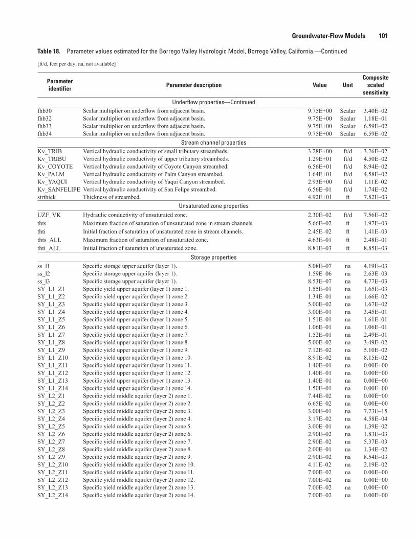
Groundwater-Flow Models 101
Table 18. Parameter values estimated for the Borrego Valley Hydrologic Model, Borrego Valley, California.—Continued
[ft/d, feet per day; na, not available]
Parameter identifier
Parameter description Value UnitComposite
scaled sensitivity
Underflow properties—Continuedfhb30 Scalar multiplier on underflow from adjacent basin. 9.75E+00 Scalar 3.40E–02fhb32 Scalar multiplier on underflow from adjacent basin. 9.75E+00 Scalar 1.18E–01fhb33 Scalar multiplier on underflow from adjacent basin. 9.75E+00 Scalar 6.59E–02fhb34 Scalar multiplier on underflow from adjacent basin. 9.75E+00 Scalar 6.59E–02
Stream channel propertiesKv_TRIB Vertical hydraulic conductivity of small tributary streambeds. 3.28E+00 ft/d 3.26E–02Kv_TRIBU Vertical hydraulic conductivity of upper tributary streambeds. 1.29E+01 ft/d 4.50E–02Kv_COYOTE Vertical hydraulic conductivity of Coyote Canyon streambed. 6.56E+01 ft/d 8.94E–02Kv_PALM Vertical hydraulic conductivity of Palm Canyon streambed. 1.64E+01 ft/d 4.58E–02Kv_YAQUI Vertical hydraulic conductivity of Yaqui Canyon streambed. 2.93E+00 ft/d 1.11E–02Kv_SANFELIPE Vertical hydraulic conductivity of San Felipe streambed. 6.56E–01 ft/d 1.74E–02strthick Thickness of streambed. 4.92E+01 ft 7.82E–03
Unsaturated zone propertiesUZF_VK Hydraulic conductivity of unsaturated zone. 2.30E–02 ft/d 7.56E–02thts Maximum fraction of saturation of unsaturated zone in stream channels. 5.66E–02 ft 1.97E–03thti Initial fraction of saturation of unsaturated zone in stream channels. 2.45E–02 ft 1.41E–03thts_ALL Maximum fraction of saturation of unsaturated zone. 4.63E–01 ft 2.48E–01thti_ALL Initial fraction of saturation of unsaturated zone. 8.81E–03 ft 8.85E–03
Storage propertiesss_l1 Specific storage upper aquifer (layer 1). 5.08E–07 na 4.19E–03ss_l2 Specific storage upper aquifer (layer 1). 1.59E–06 na 2.63E–03ss_l3 Specific storage upper aquifer (layer 1). 8.53E–07 na 4.77E–03SY_L1_Z1 Specific yield upper aquifer (layer 1) zone 1. 1.55E–01 na 1.65E–03SY_L1_Z2 Specific yield upper aquifer (layer 1) zone 2. 1.34E–01 na 1.66E–02SY_L1_Z3 Specific yield upper aquifer (layer 1) zone 3. 5.00E–02 na 1.67E–02SY_L1_Z4 Specific yield upper aquifer (layer 1) zone 4. 3.00E–01 na 3.45E–01SY_L1_Z5 Specific yield upper aquifer (layer 1) zone 5. 1.51E–01 na 1.61E–01SY_L1_Z6 Specific yield upper aquifer (layer 1) zone 6. 1.06E–01 na 1.06E–01SY_L1_Z7 Specific yield upper aquifer (layer 1) zone 7. 1.52E–01 na 2.49E–01SY_L1_Z8 Specific yield upper aquifer (layer 1) zone 8. 5.00E–02 na 3.49E–02SY_L1_Z9 Specific yield upper aquifer (layer 1) zone 9. 7.12E–02 na 5.10E–02SY_L1_Z10 Specific yield upper aquifer (layer 1) zone 10. 8.91E–02 na 8.15E–02SY_L1_Z11 Specific yield upper aquifer (layer 1) zone 11. 1.40E–01 na 0.00E+00SY_L1_Z12 Specific yield upper aquifer (layer 1) zone 12. 1.40E–01 na 0.00E+00SY_L1_Z13 Specific yield upper aquifer (layer 1) zone 13. 1.40E–01 na 0.00E+00SY_L1_Z14 Specific yield upper aquifer (layer 1) zone 14. 1.50E–01 na 0.00E+00SY_L2_Z1 Specific yield middle aquifer (layer 2) zone 1. 7.44E–02 na 0.00E+00SY_L2_Z2 Specific yield middle aquifer (layer 2) zone 2. 6.65E–02 na 0.00E+00SY_L2_Z3 Specific yield middle aquifer (layer 2) zone 3. 3.00E–01 na 7.73E–15SY_L2_Z4 Specific yield middle aquifer (layer 2) zone 4. 3.17E–02 na 4.58E–04SY_L2_Z5 Specific yield middle aquifer (layer 2) zone 5. 3.00E–01 na 1.39E–02SY_L2_Z6 Specific yield middle aquifer (layer 2) zone 6. 2.90E–02 na 1.83E–03SY_L2_Z7 Specific yield middle aquifer (layer 2) zone 7. 2.90E–02 na 5.37E–03SY_L2_Z8 Specific yield middle aquifer (layer 2) zone 8. 2.00E–01 na 1.34E–02SY_L2_Z9 Specific yield middle aquifer (layer 2) zone 9. 2.90E–02 na 8.54E–03SY_L2_Z10 Specific yield middle aquifer (layer 2) zone 10. 4.11E–02 na 2.19E–02SY_L2_Z11 Specific yield middle aquifer (layer 2) zone 11. 7.00E–02 na 0.00E+00SY_L2_Z12 Specific yield middle aquifer (layer 2) zone 12. 7.00E–02 na 0.00E+00SY_L2_Z13 Specific yield middle aquifer (layer 2) zone 13. 7.00E–02 na 0.00E+00SY_L2_Z14 Specific yield middle aquifer (layer 2) zone 14. 7.00E–02 na 0.00E+00
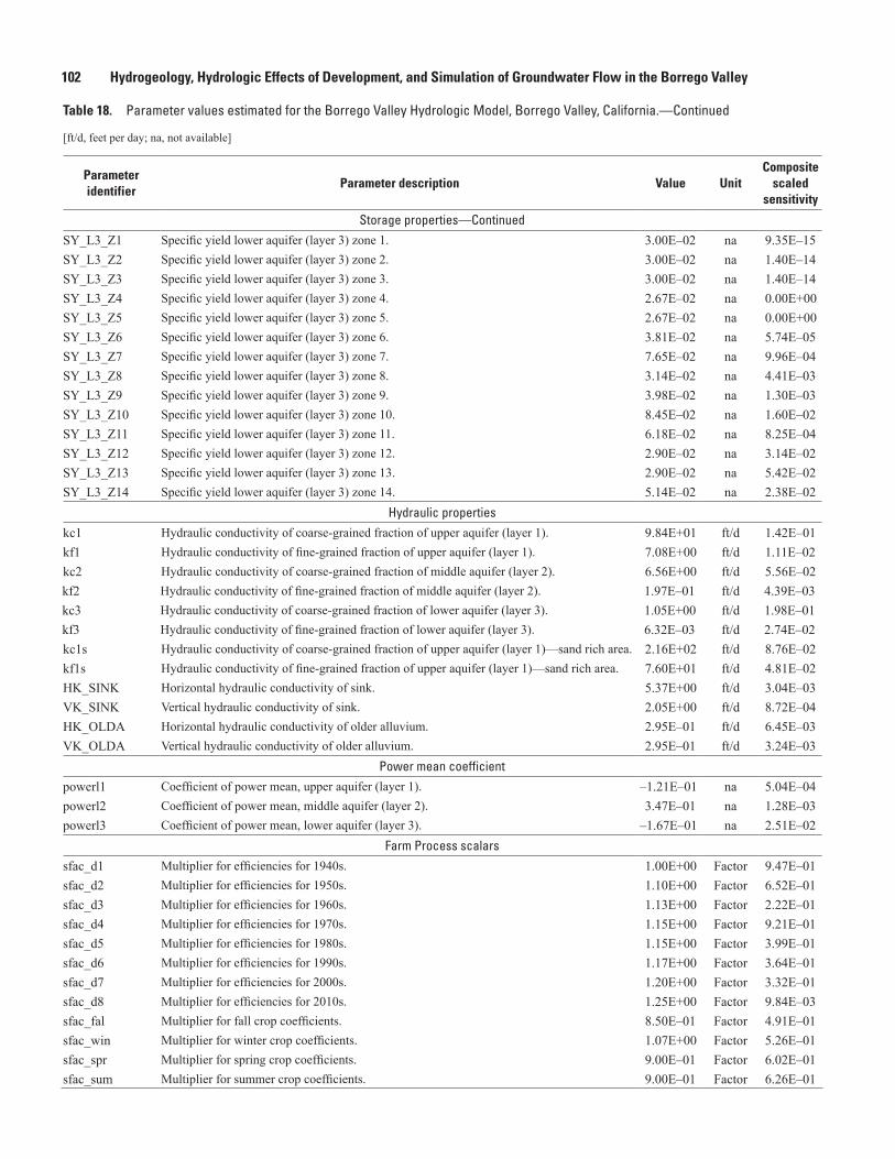
102 Hydrogeology, Hydrologic Effects of Development, and Simulation of Groundwater Flow in the Borrego Valley
Table 18. Parameter values estimated for the Borrego Valley Hydrologic Model, Borrego Valley, California.—Continued
[ft/d, feet per day; na, not available]
Parameter identifier
Parameter description Value UnitComposite
scaled sensitivity
Storage properties—ContinuedSY_L3_Z1 Specific yield lower aquifer (layer 3) zone 1. 3.00E–02 na 9.35E–15SY_L3_Z2 Specific yield lower aquifer (layer 3) zone 2. 3.00E–02 na 1.40E–14SY_L3_Z3 Specific yield lower aquifer (layer 3) zone 3. 3.00E–02 na 1.40E–14SY_L3_Z4 Specific yield lower aquifer (layer 3) zone 4. 2.67E–02 na 0.00E+00SY_L3_Z5 Specific yield lower aquifer (layer 3) zone 5. 2.67E–02 na 0.00E+00SY_L3_Z6 Specific yield lower aquifer (layer 3) zone 6. 3.81E–02 na 5.74E–05SY_L3_Z7 Specific yield lower aquifer (layer 3) zone 7. 7.65E–02 na 9.96E–04SY_L3_Z8 Specific yield lower aquifer (layer 3) zone 8. 3.14E–02 na 4.41E–03SY_L3_Z9 Specific yield lower aquifer (layer 3) zone 9. 3.98E–02 na 1.30E–03SY_L3_Z10 Specific yield lower aquifer (layer 3) zone 10. 8.45E–02 na 1.60E–02SY_L3_Z11 Specific yield lower aquifer (layer 3) zone 11. 6.18E–02 na 8.25E–04SY_L3_Z12 Specific yield lower aquifer (layer 3) zone 12. 2.90E–02 na 3.14E–02SY_L3_Z13 Specific yield lower aquifer (layer 3) zone 13. 2.90E–02 na 5.42E–02SY_L3_Z14 Specific yield lower aquifer (layer 3) zone 14. 5.14E–02 na 2.38E–02
Hydraulic propertieskc1 Hydraulic conductivity of coarse-grained fraction of upper aquifer (layer 1). 9.84E+01 ft/d 1.42E–01kf1 Hydraulic conductivity of fine-grained fraction of upper aquifer (layer 1). 7.08E+00 ft/d 1.11E–02kc2 Hydraulic conductivity of coarse-grained fraction of middle aquifer (layer 2). 6.56E+00 ft/d 5.56E–02kf2 Hydraulic conductivity of fine-grained fraction of middle aquifer (layer 2). 1.97E–01 ft/d 4.39E–03kc3 Hydraulic conductivity of coarse-grained fraction of lower aquifer (layer 3). 1.05E+00 ft/d 1.98E–01kf3 Hydraulic conductivity of fine-grained fraction of lower aquifer (layer 3). 6.32E–03 ft/d 2.74E–02kc1s Hydraulic conductivity of coarse-grained fraction of upper aquifer (layer 1)—sand rich area. 2.16E+02 ft/d 8.76E–02kf1s Hydraulic conductivity of fine-grained fraction of upper aquifer (layer 1)—sand rich area. 7.60E+01 ft/d 4.81E–02HK_SINK Horizontal hydraulic conductivity of sink. 5.37E+00 ft/d 3.04E–03VK_SINK Vertical hydraulic conductivity of sink. 2.05E+00 ft/d 8.72E–04HK_OLDA Horizontal hydraulic conductivity of older alluvium. 2.95E–01 ft/d 6.45E–03VK_OLDA Vertical hydraulic conductivity of older alluvium. 2.95E–01 ft/d 3.24E–03
Power mean coefficientpowerl1 Coefficient of power mean, upper aquifer (layer 1). –1.21E–01 na 5.04E–04powerl2 Coefficient of power mean, middle aquifer (layer 2). 3.47E–01 na 1.28E–03powerl3 Coefficient of power mean, lower aquifer (layer 3). –1.67E–01 na 2.51E–02
Farm Process scalarssfac_d1 Multiplier for efficiencies for 1940s. 1.00E+00 Factor 9.47E–01sfac_d2 Multiplier for efficiencies for 1950s. 1.10E+00 Factor 6.52E–01sfac_d3 Multiplier for efficiencies for 1960s. 1.13E+00 Factor 2.22E–01sfac_d4 Multiplier for efficiencies for 1970s. 1.15E+00 Factor 9.21E–01sfac_d5 Multiplier for efficiencies for 1980s. 1.15E+00 Factor 3.99E–01sfac_d6 Multiplier for efficiencies for 1990s. 1.17E+00 Factor 3.64E–01sfac_d7 Multiplier for efficiencies for 2000s. 1.20E+00 Factor 3.32E–01sfac_d8 Multiplier for efficiencies for 2010s. 1.25E+00 Factor 9.84E–03sfac_fal Multiplier for fall crop coefficients. 8.50E–01 Factor 4.91E–01sfac_win Multiplier for winter crop coefficients. 1.07E+00 Factor 5.26E–01sfac_spr Multiplier for spring crop coefficients. 9.00E–01 Factor 6.02E–01sfac_sum Multiplier for summer crop coefficients. 9.00E–01 Factor 6.26E–01
Groundwater-Flow Models 103
Initial input parameters were specified within ranges of reasonable values. A combination of PEST (Doherty, 2010a, b, c; Doherty and Hunt, 2010) and manual adjustments were used in the parameter estimation and sensitivity analyses to derive the estimated parameter values that resulted in best fits of simulated head values to the calibration targets and that reasonably reflected the hydrologic conditions measured in the aquifer system, including measured groundwater-level elevations and associated long-term trends as well as estimated discharge. Although a number of parameters were estimated during calibration (table 18 and list in previous paragraph), a summary of some of the more critical parameters follows.
As described in the “Calculation of Hydraulic Properties” section of this report, Kh and Kv were estimated for every cell in the BVHM on the basis of sediment texture and end-member K values (Kc and Kf) by using the averaging method (weighted arithmetic average for Kh; power mean for Kv). These end-member K values and the p value used in the power mean were adjusted by using PEST to minimize model error. During initial calibration efforts, the same end-member Ks and p were used for the entire valley. As calibration progressed, it became evident that more hydraulic parameters were necessary to represent the system with sufficient accuracy. Values of Kc and Kf were then defined separately for each of the aquifers, accounting for differences in their depositional environments. Separate p values were also used for each of the aquifers. The estimated end-member K for each aquifer was somewhat different; the Kv also differed according to the power mean and the end-member K (table 18). Several specific-yield values defined by zones generally representing groupings of similar percentage of coarse-grained deposits (fig. 36) were adjusted during calibration.
The streambed Kv parameters also were estimated. Six streambed Kv zones were identified (fig. 37), and low streambed Kvs were used as initial estimates, then adjusted during calibration (table 18). In addition, scalar multipliers were estimated to adjust the total amount of flow into the system from the BCM-simulated runoff and underflow from the adjacent basins. HYDMOD, a program for extracting time-series data from MODFLOW (Hanson and Leake, 1998), was used to examine surface-water flow at downstream points around the Borrego Sink and flow exiting the model along San Felipe Creek. Although the magnitude of these surface-water flows is unknown, during extremely wet periods, stormwater has often reached the Borrego Sink and flowed out of the basin along San Felipe Creek. Streambed properties were constrained so that the simulated flows occurred periodically during wet events and not continually throughout the simulation.
Observation DataThe ability of the transient hydrologic flow model to
simulate data accurately that agree with observation data was evaluated. Observations are groundwater-level measurements
obtained in the field and estimated or measured pumpage. Calibration adjustments were related to the combined fitting of the groundwater levels, groundwater-level differences over time, and pumpage observations (fig. 41). A comparison of the simulated values to observed values for pumpage was done to assess the capacity of the model to simulate the effects of changing stresses on the hydrologic system reasonably over time. The comparison provided a measure of model performance over various historical time intervals. The resulting error distributions constrained the parameter set, and the comparison between observed and simulated values provided a basis for sensitivity analysis of selected parameters. Details on this comparison are summarized in the section “Calibration Procedure.” Furthermore, an overall estimate of model fit was made by using the groundwater-level data. Because of the large number of variables adjusted as part of model calibration, as well as assumptions and simplifications made in the development of the BVHM, there could be significant uncertainties and limitations in the application of the model. These uncertainties and model limitations are discussed later in this report in the section “Model Uncertainty, Limitations, and Improvements.”
The largest suite of observation values used for calibration consisted of groundwater levels and changes in groundwater levels over time. BWD maintains a database of key wells in the Borrego Valley in which groundwater levels are regularly measured as part of the monitoring network. The USGS NWIS database also has historical groundwater-level measurements. In addition, CA-DWR routinely measures groundwater levels in the Borrego Valley. These data were combined to form a database of available groundwater levels throughout the Borrego Valley from 1945 to 2010; 2,224 groundwater-level measurements in 73 single- and multiple-aquifer wells were used for model calibration (fig. 41). For calibration, measured water levels were compared with the simulated water levels from the model row and column in which the well was located and the model layer in which the well was screened (well interval open to the aquifer system). Water levels for a well that was screened through multiple model layers were compared to the corresponding average (thickness-weighted) of the simulated water levels in all of these layers. Measured water levels were used in two ways—as direct observations of groundwater level and as observations of drawdown. For the drawdown data, it was assumed that the first groundwater-level measurement in a well is the reference value; that is, subsequent drawdown is calculated as deviations from the first value. Drawdown data were used in this study to emphasize in the calibration the importance of relative changes in water levels over time. Such processing of raw observation data, in this case drawdowns, can potentially add information that increases the signal-to-noise ratio of the observation dataset (Westenbroek and others, 2012). Hydrographs for selected observation wells are shown in figure 42.
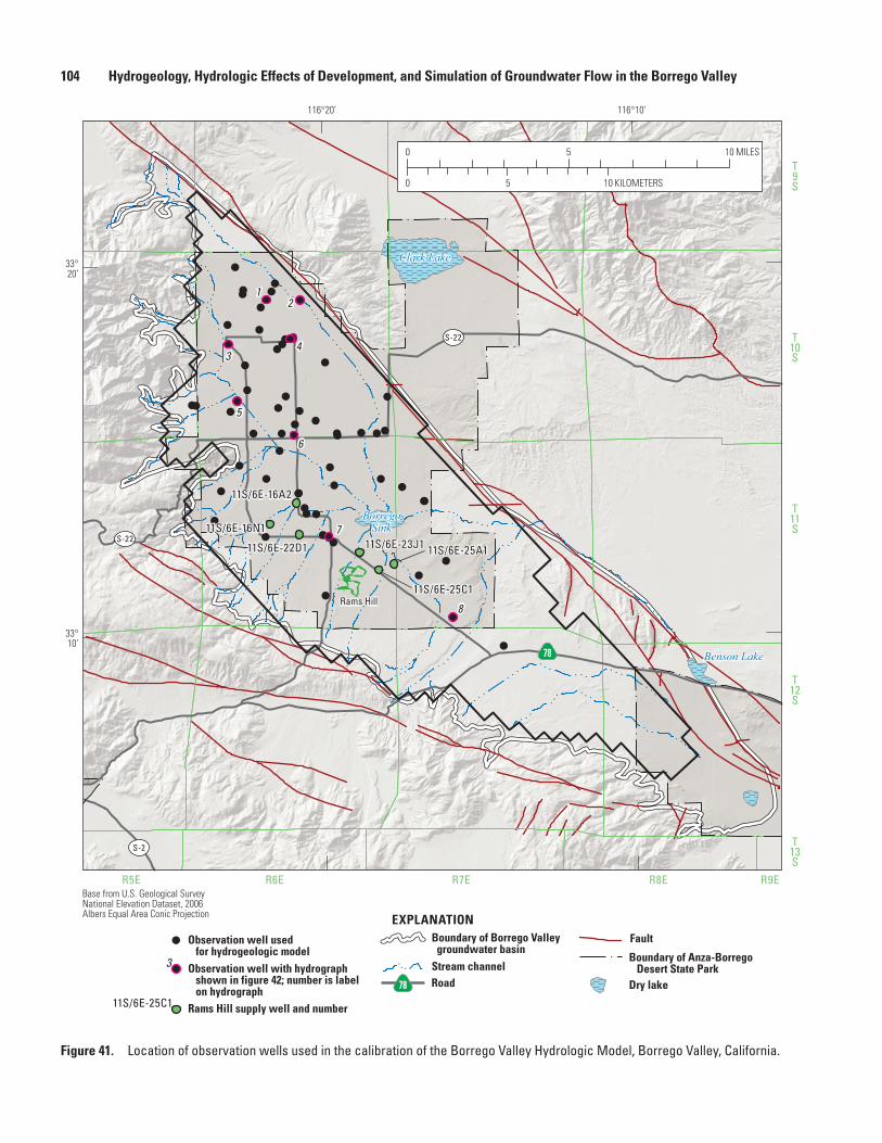
104 Hydrogeology, Hydrologic Effects of Development, and Simulation of Groundwater Flow in the Borrego Valley
Clark Lake
BorregoSink
Benson Lake
T9S
T10S
T11S
T12S
T13S
R5E R6E R7E R8E R9EBase from U.S. Geological Survey National Elevation Dataset, 2006Albers Equal Area Conic Projection
S-22
S-22
S-2
78
11S/6E-16A2
11S/6E-16N1
11S/6E-22D1 11S/6E-23J1 11S/6E-25A1
11S/6E-25C1
34
5
6
7
8
12
116°10’116°20’
33°20’
33°10’
0
0 5 10
5 10 MILES
KILOMETERS
sac13-0509_Figure 41 hobs sites
Rams Hill
EXPLANATIONObservation well used for hydrogeologic model
11S/6E-25C1 Rams Hill supply well and number
Observation well with hydrograph shown in figure 42; number is label on hydrograph
3 Stream channel
Boundary of Borrego Valley groundwater basin
Road78
Boundary of Anza-Borrego Desert State Park
Fault
Dry lake
Figure 41. Location of observation wells used in the calibration of the Borrego Valley Hydrologic Model, Borrego Valley, California.
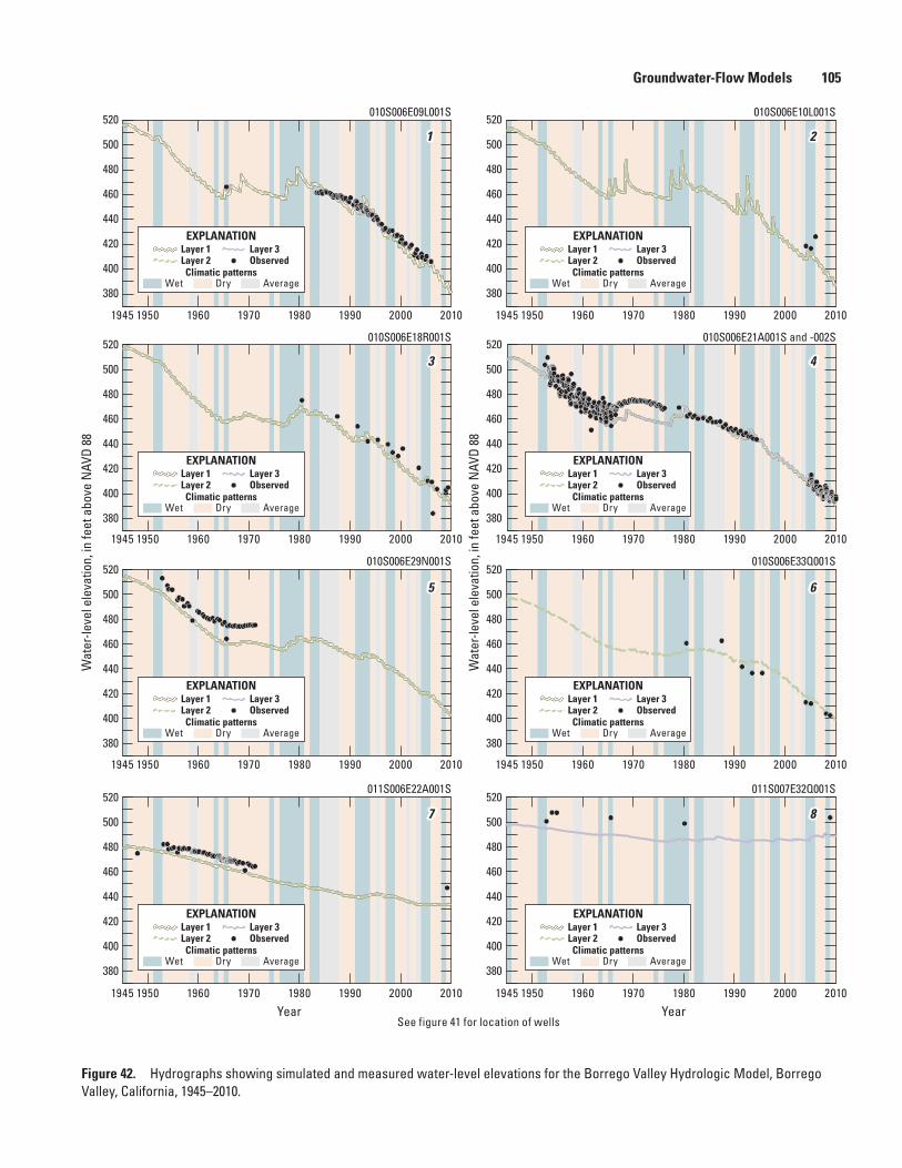
Groundwater-Flow Models 105
sac13-0509_fig42_updated
1945 1950 1960 1970 1980 1990 2000 2010
Year1945 1950 1960 1970 1980 1990 2000 2010
Year
1945 1950 1960 1970 1980 1990 2000 2010 1945 1950 1960 1970 1980 1990 2000 2010
1945 1950 1960 1970 1980 1990 2000 2010 1945 1950 1960 1970 1980 1990 2000 2010
1945 1950 1960 1970 1980 1990 2000 2010 1945 1950 1960 1970 1980 1990 2000 2010
1
3
5
7
2
4
6
8
Wat
er-le
vel e
leva
tion,
in fe
et a
bove
NAV
D 88
Wat
er-le
vel e
leva
tion,
in fe
et a
bove
NAV
D 88
See figure 41 for location of wells
400
420
440
460
480
380
500
520
400
420
440
460
480
380
500
520
400
420
440
460
480
380
500
520
400
420
440
460
480
380
500
520
400
420
440
460
480
380
500
520
400
420
440
460
480
380
500
520
400
420
440
460
480
380
500
520
400
420
440
460
480
380
500
520
EXPLANATION
ObservedLayer 1Layer 2
Layer 3
Climatic patternsWet Dry Average
EXPLANATION
ObservedLayer 1Layer 2
Layer 3
Climatic patternsWet Dry Average
EXPLANATION
ObservedLayer 1Layer 2
Layer 3
Climatic patternsWet Dry Average
EXPLANATION
ObservedLayer 1Layer 2
Layer 3
Climatic patternsWet Dry Average
EXPLANATION
ObservedLayer 1Layer 2
Layer 3
Climatic patternsWet Dry Average
EXPLANATION
ObservedLayer 1Layer 2
Layer 3
Climatic patternsWet Dry Average
EXPLANATION
ObservedLayer 1Layer 2
Layer 3
Climatic patternsWet Dry Average
EXPLANATION
ObservedLayer 1Layer 2
Layer 3
Climatic patternsWet Dry Average
010S006E10L001S
010S006E21A001S and -002S
010S006E33Q001S
011S007E32Q001S
010S006E09L001S
010S006E18R001S
010S006E29N001S
011S006E22A001S
Figure 42. Hydrographs showing simulated and measured water-level elevations for the Borrego Valley Hydrologic Model, Borrego Valley, California, 1945–2010.
106 Hydrogeology, Hydrologic Effects of Development, and Simulation of Groundwater Flow in the Borrego Valley
RegularizationMany techniques in parameter-estimation theory provide
systematic methods for dealing with under-determined parameter-estimation problems. These techniques are generally referred to as regularization techniques (Hunt and others, 2007). Tikhonov regularization (Tikhonov and Arsenin, 1977; Doherty, 2003) is provided in the PEST software and was used in this study.
Tikhonov regularization is a form of Bayesian estimation in which a composite objective function is minimized (Yeh, 1986). This composite objective function consists of the standard measurement objective function and a “penalty term” that penalizes the composite objective function when parameters deviate from their preferred or expected value, which is based on prior information. The combined objective function is represented by the following equation:
Φ Φ Φ= + r m (4)
where Φ is the composite or overall objective function, Φr is the penalty function for parameter
deviations from expected values, Φm is the least-squares objective function, and µ is the trade-off or regularization weighting
factor. Tikhonov regularization determines the optimal
regularization weighting factor, µ, given a modeler-specified level of calibration, that is, a desired value for Φm, denoted as Φm
1 . Therefore, the inverse problem is considered to have converged when Φ Φm m≤ 1 ; however, in practice it is often the case that Φ Φm m≈ 1 . In the PEST software used here, the Tikhonov regularization algorithm determines the optimal µ such that Φr is minimized (Doherty, 2003).
Prior estimates of model parameters for input into the BVHM were assigned, for the most part, by using values reported in Mitten and others (1988) and Henderson (2001). Additional parameters resulting from modifications to their models were assigned values on the basis of professional judgment and knowledge of the area. Initial estimates for recharge were obtained from the results of the BCM presented in this report and the results of Mitten and others (1988) and Henderson (2001). Other model parameters, for which no prior information was available, were assigned values similar to those of nearby parameters of the same types for which some information was available. This approach for assigning parameter values tends toward the use of a simpler model parameterization by interjecting a precondition for local homogeneity.
The preliminary regularized PEST results indicate that some of the values used for prior information appeared to be incorrect. For example, the assumption of homogeneity was slightly erroneous, or the assigned values were slightly erroneous. Therefore, the prior or initial values of these parameters were modified to reflect the trends toward
higher or lower values of the erroneous parameter values, as indicated by the iterative estimation process. This iterative process of minimizing the composite objective function (equation 4) with a value set for Φm
1 in PEST, then changing the target parameter values slightly and using PEST again to minimize the composite objective function, was repeated until a subjective desired level of calibration was achieved, while maintaining parameter values that were consistent with the hydrogeologic conceptualization of the region. For each attempt at calibrating the model, Tikhonov regularization was employed with an appropriate value set for Φm
1 . A regularization group was defined in PEST for each parameter group. The final calibrated parameter values are listed in table 18.
Tikhonov regularization provides the means to estimate all model parameters regardless of parameter sensitivity to the observations used for calibration. Therefore, in this report, all 115 parameters in the BVHM were estimated by using PEST with Tikhonov regularization, in which a prior or target value is assigned to each parameter. The calibrated parameter values and their composite sensitivities, as computed by PEST (Doherty, 2010a, chap. 5, p. 5–16), are listed in table 18. Note that these composite sensitivities were computed by using only the relations between the parameters and the model outputs that correspond to the observation data; that is, the regularization component was not included in this calculation.
The overall model fit for water-level comparisons is generally good when the simulated head values are compared against the measured groundwater levels. About 90 percent of the residuals were between −20 and +20 ft, and more than 50 percent were between −5 and 5 ft (fig. 43). Simulated groundwater levels closely matched measured groundwater levels and showed essentially no bias, as indicated by an average residual of 0.1 ft and the relatively small magnitude of most of the residuals. Overall, the residuals tended to underestimate groundwater levels slightly (positive residuals). The residuals ranged from −100 to 53 ft (observed minus simulated; figs. 43, 44), and the standard deviation and root mean square error (RMSE) were both approximately 11 ft. However, there are some extremely negative residuals, which are considered an artifact of some of the groundwater levels representing pumping conditions in the well rather than a static condition. The total change in measured groundwater levels in wells ranged from −140 ft to slight rises in local areas. In the plot of simulated in relation to measured groundwater levels in figure 44, the outliers show an overestimation of measured groundwater levels at the lowest water-level elevations.
Hydrographs comparing simulated and measured groundwater levels for selected wells illustrate the match of groundwater levels throughout system (fig. 42). The minimum period over which model simulations can accurately reproduce fluctuations in the groundwater-flow system (the response time of the model) varies with the depth to groundwater, hydrologic setting, hydraulic properties, climate, and land use. The amplitude of monthly fluctuations in simulated heads is generally greater than that of fluctuations in measured
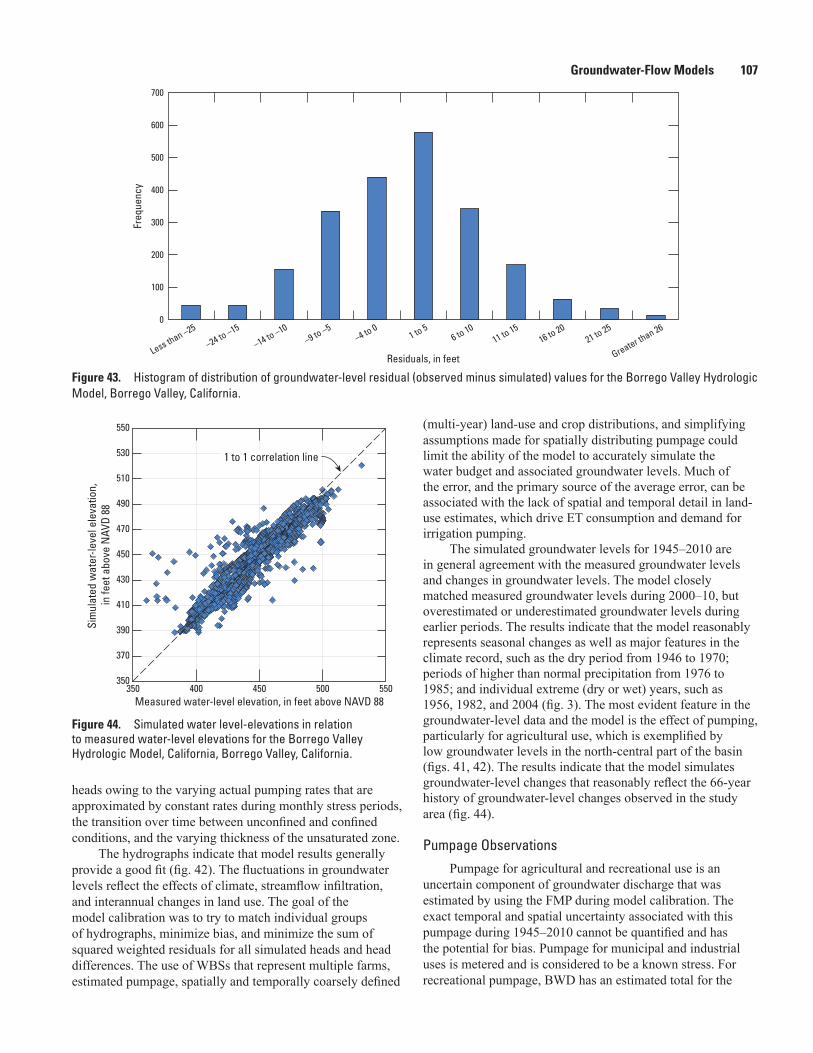
Groundwater-Flow Models 107
heads owing to the varying actual pumping rates that are approximated by constant rates during monthly stress periods, the transition over time between unconfined and confined conditions, and the varying thickness of the unsaturated zone.
The hydrographs indicate that model results generally provide a good fit (fig. 42). The fluctuations in groundwater levels reflect the effects of climate, streamflow infiltration, and interannual changes in land use. The goal of the model calibration was to try to match individual groups of hydrographs, minimize bias, and minimize the sum of squared weighted residuals for all simulated heads and head differences. The use of WBSs that represent multiple farms, estimated pumpage, spatially and temporally coarsely defined
(multi-year) land-use and crop distributions, and simplifying assumptions made for spatially distributing pumpage could limit the ability of the model to accurately simulate the water budget and associated groundwater levels. Much of the error, and the primary source of the average error, can be associated with the lack of spatial and temporal detail in land-use estimates, which drive ET consumption and demand for irrigation pumping.
The simulated groundwater levels for 1945–2010 are in general agreement with the measured groundwater levels and changes in groundwater levels. The model closely matched measured groundwater levels during 2000–10, but overestimated or underestimated groundwater levels during earlier periods. The results indicate that the model reasonably represents seasonal changes as well as major features in the climate record, such as the dry period from 1946 to 1970; periods of higher than normal precipitation from 1976 to 1985; and individual extreme (dry or wet) years, such as 1956, 1982, and 2004 (fig. 3). The most evident feature in the groundwater-level data and the model is the effect of pumping, particularly for agricultural use, which is exemplified by low groundwater levels in the north-central part of the basin (figs. 41, 42). The results indicate that the model simulates groundwater-level changes that reasonably reflect the 66-year history of groundwater-level changes observed in the study area (fig. 44).
Pumpage ObservationsPumpage for agricultural and recreational use is an
uncertain component of groundwater discharge that was estimated by using the FMP during model calibration. The exact temporal and spatial uncertainty associated with this pumpage during 1945–2010 cannot be quantified and has the potential for bias. Pumpage for municipal and industrial uses is metered and is considered to be a known stress. For recreational pumpage, BWD has an estimated total for the
Figure 43. Histogram of distribution of groundwater-level residual (observed minus simulated) values for the Borrego Valley Hydrologic Model, Borrego Valley, California.
Figure 44. Simulated water level-elevations in relation to measured water-level elevations for the Borrego Valley Hydrologic Model, California, Borrego Valley, California.
sac13-0509_fig43
fig. 43 residual Histogram
0
100
200
300
400
500
600
700
Less than –25
–24 to –15
–14 to –10–9 to –5
–4 to 01 to 5
Residuals, in feet
6 to 1011 to 15
16 to 2021 to 25
Greater than 26
Freq
uenc
y
sac13-0509_fig44
fig. 44, Observed vs. Simulated
350
370
390
410
430
450
470
490
510
530
550
350 400 450 500 550
Sim
ulat
ed w
ater
-leve
l ele
vatio
n,
in fe
et a
bove
NAV
D 88
Measured water-level elevation, in feet above NAVD 88
1 to 1 correlation line
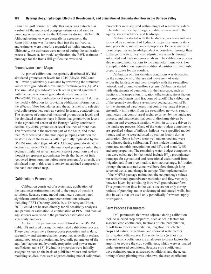
108 Hydrogeology, Hydrologic Effects of Development, and Simulation of Groundwater Flow in the Borrego Valley
Rams Hill golf course. Initially, this usage was extracted as a subset of the municipal pumpage estimates and used as pumpage observations for the 336 months during 1983–2010. Although estimates were generally in agreement, the Rams Hill usage was for more than just the golf course, and estimates were therefore regarded as highly uncertain. Ultimately, the estimates were not used during the calibration process. However, for model application, the BWD estimate of pumpage for the Rams Hill golf course was used.
Groundwater-Level MapsAs part of calibration, the spatially distributed BVHM-
simulated groundwater levels for 1945 (Moyle, 1982) and 2010 were qualitatively evaluated by reviewing the simulated values with groundwater-level maps for those years (fig. 45). The simulated groundwater levels are in general agreement with the hand-contoured groundwater-level maps for 1945–2010. The groundwater-level maps were useful during the model calibration for providing additional information on the effects of flow boundaries and the adjustments to selected hydraulic properties, such as vertical hydraulic conductivities. The sequence of contoured measured groundwater levels and the simulated thematic maps indicate that groundwater levels in the agricultural center of the Borrego Valley continue to decline. By 2010, groundwater-level declines of more than 120 ft persisted in the northern part of the basin, and more than 75 ft persisted in the municipal pumping center on the western side of the basin, a pattern partially replicated by the BVHM simulation (figs. 44, 45). Although groundwater-level declines exceeded 75 ft in the municipal pumping center, these declines might not reflect ambient (static) conditions and are thought to represent groundwater levels that have not fully recovered from pumping before measurement. As a result, the simulated map in this area is somewhat subdued compared to the hand-contoured map.
Calibration Procedure
Calibration consisted of a systematic application of the parameter estimation method to the range of possible solutions. Because some model parameters demonstrated significant correlations, parameter estimation software, including PEST (Doherty, 2010a, b, c; Doherty and Hunt, 2010), could not be used directly for all sensitivity analyses and parameter estimation. A combination of PEST and manual adjustments were used in the parameter estimation and sensitivity analyses.
A total of 137 parameters were defined in the BVHM (table 18) and used during the automated calibration process. These parameters were farm-process properties and scalars, streamflow and stream-channel properties, underflow scalars, unsaturated-zone properties, and hydraulic parameters of the aquifers (storage and hydraulic properties and power mean coefficients; table 18). Hydraulic properties were initially assigned values on the basis of published values and earlier modeling studies, then were adjusted during model calibration.
Parameters were adjusted within ranges of reasonable values to best-fit historical hydrologic conditions measured in the aquifer, stream network, and landscape.
Calibration started with the landscape processes and was followed by adjustment of hydraulic properties, unsaturated-zone properties, and streambed properties. Because many of these properties are head-dependent or correlated through their exchange of water, they were adjusted recursively through automated and trial-and-error analysis. The calibration process also required modifications to the parameter framework. For example, calibration required additional partitions of hydraulic property zones for the aquifers.
Calibration of transient-state conditions was dependent on the components of the use and movement of water across the landscape and their interplay with the streamflow network and groundwater-flow system. Calibration started with adjustments of parameters in the landscape, such as fractions of transpiration, irrigation efficiencies, stress factors for crop coefficients, and fractions of runoff. The calibration of the groundwater-flow system involved adjustment of Kv for the streambed parameters that control recharge driven by streamflow infiltration from the streamflow network, runoff parameters that control areal recharge driven by the landscape process, and parameters that control discharge driven by pumping and evapotranspiration, which, in turn, are driven by the landscape process. Many of the water-budget components are specified values of inflows. Inflows were specified model inputs, and some were adjusted by scaling factors during calibration. Some inflows were well understood and were not adjusted during calibration. These include municipal pumpage, monthly precipitation and ETo, and many WBS and crop properties. The remaining water-budget components that were calculated by the model include ETact, groundwater pumpage for agricultural and recreational uses, runoff from irrigation and from precipitation, farm net recharge, infiltration through the unsaturated zone, wellbore flow through long-screened wells, and change in storage. The implementation of the MNW2 package maintained the net pumpage values, but redistributed groundwater extraction and flow vertically between layers by simulating intra-well groundwater flow. This groundwater flow in the wells occurs not only during periods of pumping and in undestroyed and unused wells, but also in wells that are used only periodically for water supply or irrigation.
Farm Process Parameters
FMP parameters that were adjusted during calibration include selected crop properties, such as scale factors for seasonal crop coefficients, fractions of total precipitation, runoff from excess precipitation, irrigation for selected crops and natural vegetation, and seasonal scale factors for irrigation efficiencies. The scale factors (scalars) for seasonal crop coefficients are analogous to stress factors that amplify or reduce the crop coefficients, which were estimated under unstressed conditions. Because crop coefficients were estimated under unstressed conditions, and the actual timing of crop planting was unknown, the crop coefficients
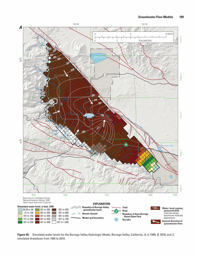
Groundwater-Flow Models 109
Clark Lake
BorregoSink
Benson Lake
T9S
T10S
T11S
T12S
T13S
R5E R6E R7E R8E R9EBase from U.S. Geological Survey National Elevation Dataset, 2006Albers Equal Area Conic Projection
S-22
S-22
S-2
78
500
520
490
480
525
530
470
535
460
510
550575
600
450
700
62585
0
520
530
116°10’116°20’
33°20’
33°10’
0
0 5 10
5 10 MILES
KILOMETERS
sac13-0509_Figure 45a 1945 WL contours
A
EXPLANATION
General direction of groundwater flow
Model-grid boundary
Stream channel
Boundary of Borrego Valley groundwater basin
Fault
Boundary of Anza-Borrego Desert State Park
Road78Water-level contour, measured 2010. Interval varies; hatchures indicate depression
490
Dry lake
Simulated water level, in feet, 194536.09 to 50
51 to 100101 to 150151 to 200201 to 250
251 to 300301 to 350351 to 400401 to 450451 to 500
501 to 550551 to 600601 to 650651 to 700
701 to 1,200
Figure 45. Simulated water levels for the Borrego Valley Hydrologic Model, Borrego Valley, California, A, in 1945; B, 2010; and C, simulated drawdown from 1945 to 2010.
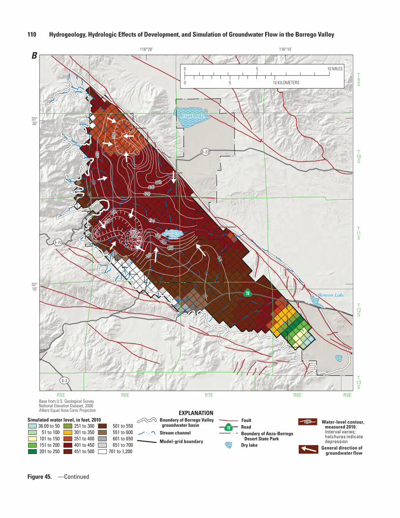
110 Hydrogeology, Hydrologic Effects of Development, and Simulation of Groundwater Flow in the Borrego Valley
Clark Lake
BorregoSink
Benson Lake
T9S
T10S
T11S
T12S
T13S
R5E R6E R7E R8E R9EBase from U.S. Geological Survey National Elevation Dataset, 2006Albers Equal Area Conic Projection
S-22
S-22
S-2
78
l
l
420
410
480
430440
400
500
460
470
450
390
380 340360 420
400
420
410
440460
380
430
390
116°10’116°20’
33°20’
33°10’
0
0 5 10
5 10 MILES
KILOMETERS
sac13-0509_Figure 45b 2010 WL Contours
B
EXPLANATIONSimulated water level, in feet, 2010
36.09 to 5051 to 100
101 to 150151 to 200201 to 250
251 to 300301 to 350351 to 400401 to 450451 to 500
501 to 550551 to 600601 to 650651 to 700
701 to 1,200General direction of groundwater flow
Model-grid boundary
Stream channel
Boundary of Borrego Valley groundwater basin
Fault
Boundary of Anza-Borrego Desert State Park
Road78Water-level contour, measured 2010. Interval varies; hatchures indicate depression
490
Dry lake
Figure 45. —Continued
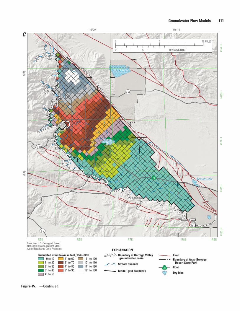
Groundwater-Flow Models 111
Clark Lake
BorregoSink
Benson Lake
T9S
T10S
T11S
T12S
T13S
R5E R6E R7E R8E R9EBase from U.S. Geological Survey National Elevation Dataset, 2006Albers Equal Area Conic Projection
S-22
S-22
S-2
78
116°10’116°20’
33°20’
33°10’
0
0 5 10
5 10 MILES
KILOMETERS
sac13-0509_Figure 45c Sim drawdown 2010
EXPLANATION
C
Simulated drawdown, in feet, 1945–2010
41 to 50
0 to 10 51 to 60 91 to 10011 to 20 61 to 70 101 to 11021 to 30 71 to 80 111 to 12031 to 40 81 to 90 121 to 130 Model-grid boundary
Stream channel
Boundary of Borrego Valley groundwater basin Boundary of Anza-Borrego
Desert State Park
Fault
Road78
Dry lake
Figure 45. —Continued
112 Hydrogeology, Hydrologic Effects of Development, and Simulation of Groundwater Flow in the Borrego Valley
required changes by a factor of 0.85 to 1.08 (table 18) to improve calibration results. Irrigation efficiencies (which include typical irrigation efficiencies and adjustments for errors in crop type, percentage of land cover, and crop distribution) were adjusted by decade to allow for changes over time, particularly for changes in irrigation practices. For simplification, it was assumed that all crops and farms changed their efficiency practices by the same factor. Irrigation efficiencies (table 16) were scaled by a factor of 1.00 to 1.25 that increases with time. Runoff from selected crops and native vegetation was added to the water available for deep percolation or for overland runoff to the streamflow network that seeps into the unsaturated zone. The fractions of losses to runoff were adjusted for native vegetation, phreatophytes, recreational areas, and various crops. Similarly, fractions of runoff from precipitation were increased to control the deep percolation and additional runoff from the native vegetation, which is the largest component of the land use in Borrego Valley.
Irrigation efficiencies were estimated for all golf courses to be 86 percent, or 14 percent irrigation return flow to the groundwater system, on the basis of results of the chloride mass-balance analysis, assuming irrigation by using a wide-area, broadcast type of sprinkler (Netto, 2001). The BVHM simulated a range of 75–94 percent (averaging 85 percent) efficiency for golf courses. Assuming citrus groves are irrigated by using a “micro sprinkler” type irrigation, Netto (2001) estimated an irrigation efficiency of 78 percent. The BVHM estimates a range of 75–98 percent (averaging 84 percent) efficiency for citrus groves. Netto (2001) estimated all other irrigation efficiency at 86 percent. In general, the BVHM estimated an average efficiency that increased over time from 75 percent to slightly greater than 90 percent, averaging about 85 percent. Note that these efficiency estimates most likely include adjustments to help simulate changes in crop coverage and type, as well as other factors affecting crop demand not specified in detail in the simulation.
Hydraulic ParametersThe model was used to estimate the values of 15
hydraulic properties, 35 storage properties, and 5 unsaturated-zone properties during model calibration. The values of Kc and Kf for each model layer were adjusted to produce simulated heads representing the long-term trends in the aquifers that best matched the measured heads and estimated streamflow losses. Because of the differences in depositional environments in the various zones within each layer, the hydraulic properties were adjusted for Kh, Kv, and storage properties (fig. 34; table 18). Other properties were estimated, including porosities; specific yields; specific storage for coarse- and fine-grained end members; and the exponent of the power mean, which is used to estimate the Kv.
The calibration of hydraulic properties required the adjustment and rescaling of these intrinsic properties on the basis of groundwater-level hydrographs (fig. 42). The most sensitive parameters were Kvs that, in part, controlled the seasonal amplitudes and differences in groundwater levels
between aquifer layers. Scaled reductions of hydraulic conductivities for selected confined zones, and scaled increases of Kv and storage properties for unconfined zones, were required. Horizontal hydraulic conductivities required more zonation in the upper and middle aquifers than in the lower aquifer (table 18). Because the model was relatively sensitive to values of specific yield, these were also split into additional zones and estimated in the automated parameter estimation.
Streamflow PropertiesAs mentioned previously, a wide rectangular channel for
the stream geometry and a constant estimation of Manning’s “n” were used for the simulations. Values for these parameters are not well known in this area and were not sensitive during calibration. The model also required calibration of the streambed Kv parameters. Groups of stream segments that stream channels were observed in the field to share characteristics, such as bed material and morphology, and which had similar size drainage basins, were represented by six parameters of streambed Kv and a parameter representing the thickness of the streambed sediments (fig. 37; table 18). The groupings and calibrated Kv values ranged from 0.65 ft/d along the armored channel of San Felipe Creek to about 65 ft/d along the gravelly channels (table 18).
Sensitivity Analysis
The BVHM was sensitive to changes in various climate and landscape properties, hydraulic and storage properties of the aquifers, and streambed vertical hydraulic conductivity. The model periodically had numerical convergence problems when some of the model parameters were perturbed too far. In some cases, this required a change to the model structure or parameter distribution. As a result, the use of systematic parameter-estimation techniques to estimate values of selected model parameters and related sensitivities that are based on perturbation approaches was augmented on the basis of guidance from sensitivity and trial-and-error analysis.
The sensitivity process in PEST identifies the sensitivity of computed values at the locations of measurements to changes in model parameters. PEST was used to identify which parameters to include in the Parameter Estimation Process (Hill and others, 2000) and to adjust the parameter values during calibration. Results of the sensitivity process indicate that the model was most sensitive to about 15 parameters related to scale factors of the crop coefficients, climate-based scale factors for runoff from precipitation and irrigation, and irrigation efficiency. The sensitivity of the parameters is shown in table 18 and figure 46. The model was most sensitive to the scaling of crop coefficients, which controls groundwater demand. The next most important parameters were the factors adjusting the amount of BCM-simulated streamflow and underflow into the basin and, therefore, the amount of recharge to the basin. The other more sensitive parameters are mostly storage properties and irrigation efficiencies.
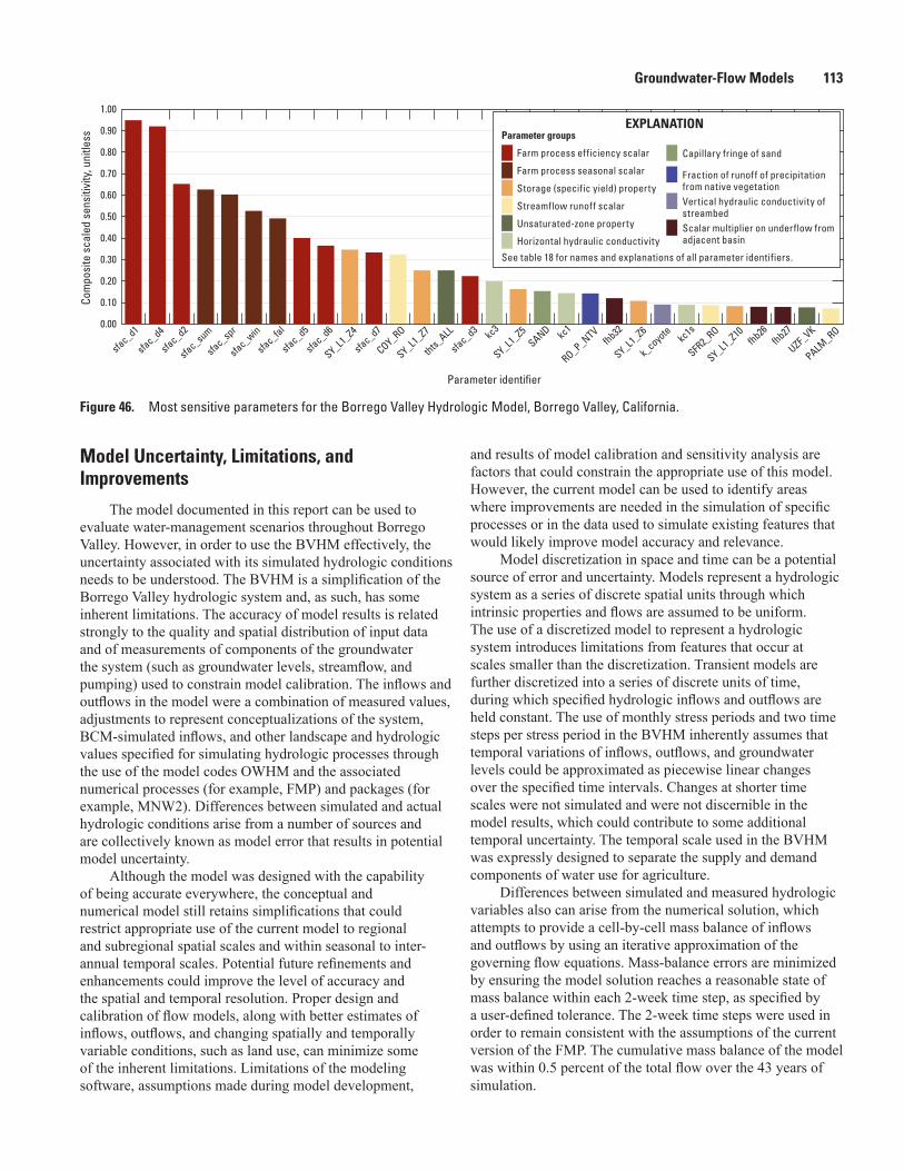
Groundwater-Flow Models 113
Model Uncertainty, Limitations, and Improvements
The model documented in this report can be used to evaluate water-management scenarios throughout Borrego Valley. However, in order to use the BVHM effectively, the uncertainty associated with its simulated hydrologic conditions needs to be understood. The BVHM is a simplification of the Borrego Valley hydrologic system and, as such, has some inherent limitations. The accuracy of model results is related strongly to the quality and spatial distribution of input data and of measurements of components of the groundwater the system (such as groundwater levels, streamflow, and pumping) used to constrain model calibration. The inflows and outflows in the model were a combination of measured values, adjustments to represent conceptualizations of the system, BCM-simulated inflows, and other landscape and hydrologic values specified for simulating hydrologic processes through the use of the model codes OWHM and the associated numerical processes (for example, FMP) and packages (for example, MNW2). Differences between simulated and actual hydrologic conditions arise from a number of sources and are collectively known as model error that results in potential model uncertainty.
Although the model was designed with the capability of being accurate everywhere, the conceptual and numerical model still retains simplifications that could restrict appropriate use of the current model to regional and subregional spatial scales and within seasonal to inter-annual temporal scales. Potential future refinements and enhancements could improve the level of accuracy and the spatial and temporal resolution. Proper design and calibration of flow models, along with better estimates of inflows, outflows, and changing spatially and temporally variable conditions, such as land use, can minimize some of the inherent limitations. Limitations of the modeling software, assumptions made during model development,
and results of model calibration and sensitivity analysis are factors that could constrain the appropriate use of this model. However, the current model can be used to identify areas where improvements are needed in the simulation of specific processes or in the data used to simulate existing features that would likely improve model accuracy and relevance.
Model discretization in space and time can be a potential source of error and uncertainty. Models represent a hydrologic system as a series of discrete spatial units through which intrinsic properties and flows are assumed to be uniform. The use of a discretized model to represent a hydrologic system introduces limitations from features that occur at scales smaller than the discretization. Transient models are further discretized into a series of discrete units of time, during which specified hydrologic inflows and outflows are held constant. The use of monthly stress periods and two time steps per stress period in the BVHM inherently assumes that temporal variations of inflows, outflows, and groundwater levels could be approximated as piecewise linear changes over the specified time intervals. Changes at shorter time scales were not simulated and were not discernible in the model results, which could contribute to some additional temporal uncertainty. The temporal scale used in the BVHM was expressly designed to separate the supply and demand components of water use for agriculture.
Differences between simulated and measured hydrologic variables also can arise from the numerical solution, which attempts to provide a cell-by-cell mass balance of inflows and outflows by using an iterative approximation of the governing flow equations. Mass-balance errors are minimized by ensuring the model solution reaches a reasonable state of mass balance within each 2-week time step, as specified by a user-defined tolerance. The 2-week time steps were used in order to remain consistent with the assumptions of the current version of the FMP. The cumulative mass balance of the model was within 0.5 percent of the total flow over the 43 years of simulation.
Figure 46. Most sensitive parameters for the Borrego Valley Hydrologic Model, Borrego Valley, California.
sac13-0509_fig46
0.00
0.10
0.20
0.30
0.40
0.50
0.60
0.70
0.80
0.90
1.00
sfac_d1
sfac_d2
sfac_su
m
sfac_sp
r
sfac_win
sfac_fal
sfac_d5
sfac_d6
SY_L1_Z4
sfac_d7
COY_RO
SY_L1_Z7
thts_ALL
sfac_d3 kc
3
SY_L1_Z5
SAND kc1
RO_P_NTVfhb32
SY_L1_Z6
k_coyo
te kc1s
SFR2_
RO
SY_L1_Z10
fhb26fhb27
UZF_VK
PALM_RO
Parameter identifier
Com
posi
te s
cale
d se
nsiti
vity
, uni
tless
sfac_d4
EXPLANATION
See table 18 for names and explanations of all parameter identifiers.
Storage (specific yield) property
Parameter groups
Unsaturated-zone property
Fraction of runoff of precipitation from native vegetation
Farm process efficiency scalar
Horizontal hydraulic conductivityScalar multiplier on underflow from adjacent basin
Streamflow runoff scalar
Farm process seasonal scalar
Capillary fringe of sand
Vertical hydraulic conductivity of streambed
114 Hydrogeology, Hydrologic Effects of Development, and Simulation of Groundwater Flow in the Borrego Valley
An additional component of model error arises from how well model-input values represent the actual hydrologic system. The accuracy of the calibrated model is contingent on the accuracy of the specified inflows and of the specified comparison flows. Model calibration provides a means to use comparisons to constrain the differences between real-world and simulated mass flows indirectly. Thus, the degree to which a simulated condition provides a reasonable representation of the hydrologic system can be evaluated by comparing simulated hydrologic conditions with those observed in the field, which in turn, provides a mass-constrained calibration. The performance and accuracy of BVHM are constrained primarily by groundwater levels; streamflows and diversions; pumping; and, to a lesser degree, streamflow losses and head differences. The model is used to develop a conceptual understanding of the flow system by quantifying the regional inflows and outflows and their relative proportions. Because the Borrego Valley flow system is inherently complex, as for all models, simplifying assumptions were made in developing and applying the numerical code OWHM. The model solves for average conditions within each 92-acre cell for each 2-week time step with the parameters interpolated or extrapolated from measurements or estimated during calibration. Thus, results from the model are most appropriate for subregional spatial scales and annual to inter-annual temporal scales for comparative analysis and generalized estimates of flows.
Several elements of the revised model remain uncertain and would require additional investigation to improve the accuracy of the simulation of groundwater and surface-water flow, the regional groundwater-storage changes, and the use and movement of water across the landscape. For example, some of the inputs to the FMP that are necessary to calculate water use remain uncertain, and model features, such as agricultural and recreational pumpages, could be sensitive to a few of these parameters, such as crop coefficients, irrigation efficiencies, multiple cropping, or monthly land use. More accurate estimates of agricultural and recreational pumpages would improve the model results. In addition, monthly or seasonal information on the distribution and change in land-use patterns would greatly increase the accuracy of the simulation. Many of the stresses that are driven by these land uses varied throughout the simulation period at higher frequencies than the lower frequency (average of about 0.2 yr−1) estimates of land use. This is evident by the improved simulation since 1992, when land-use estimates used in the model were more frequent. These variations also are driven by climatic conditions and growing periods. Hence, the changes appear seasonally and by climatic-driven events that can be yearly or multi-year in length. Because the land use was based on a generalized classification for the early years and selected crop categories, some of the agricultural composite crop classes were replaced with the composite crop of identical extent from the most recent land-use map. For example, where only cropland was specified, the interpreted composite crops were embedded. This assumes the farmer would be growing the same type of crop in a given area over the time frame of the hydrologic simulation when that land-use map was used. In some cases, such as orchards, this is generally a good
assumption; in other cases, the crops could have changed several times during the years represented by the land-use map. This is an aspect that could use much improvement in future refinements of the model. Simulating future conditions is inexact because estimates of most input data are uncertain for future years and could be better delineated in terms of their relation to climate changes. Natural vegetation, including phreatophytes, represents between 75 and 100 percent of the land use and, as such, is critical for estimating the runoff and recharge in Borrego Valley.
Some inflows, such as ungaged streamflow remain relatively uncertain, and the model could potentially benefit from improved estimates if additional capture of local runoff is a primary component of any revised BMP. Although estimation of the ungaged streamflow or linkage to a model that specifically routes streamflow and simulates recharge from the tributary drainage areas was outside the scope of this study, this could improve modeling of the streamflow network and the simulation of streamflow infiltration in the mountain-front regions.
Model uncertainty could be reduced by using additional field estimates, such as horizontal and vertical hydraulic conductivities and storage properties. Additional estimates of Kh could be obtained by using slug tests at observation-well sites or specific-capacity approximations from single-aquifer supply wells to constrain the model properties further.
In general, the textural database is more certain for the upper aquifer and the upper part of the middle aquifer and less certain for parts of the lower middle and lower aquifers. The difference between simulated and measured heads generally increases with depth below the land surface. This could reflect the decreasing accuracy of textural data, which were used to estimate the hydraulic conductivities, with increasing depth below the land surface. The information for the lower aquifer could be especially uncertain, because few wells currently produce from this unit in the Borrego Valley.
Several of the processes in the model potentially could allow for refined simulation of selected flow features. Improved modeling of multi-aquifer wells to account for better estimates of actual pumping capacities of all wells could increase the accuracy of simulated pumpage. Similarly, the simulation of runoff within the FMP could be enhanced to better simulate the intensity of wet-year winter precipitation events, which would facilitate better estimates of runoff. Antecedent soil moisture is not accounted for by FMP. This could cause underestimation of runoff during the wet years along with overestimation of the unsatisfied crop demand used to drive the simulated pumping.
A hydrologic flow model is a valuable tool for testing the conceptualization of the hydrologic system and for predicting the response of the system to changes in aquifer stresses. However, a model is only an approximation of the actual aquifer system and, therefore, does not exactly represent the actual system. The model relies on estimates of aquifer properties and stresses, which have some degree of uncertainty. Although some of this uncertainty has been evaluated in this work, the model still lacks the small-scale spatial and temporal variability present in the actual system.
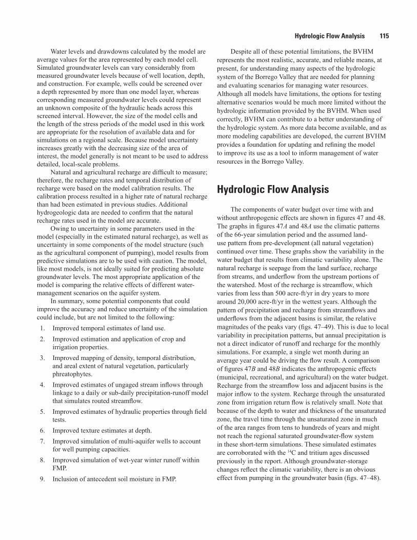
Hydrologic Flow Analysis 115
Water levels and drawdowns calculated by the model are average values for the area represented by each model cell. Simulated groundwater levels can vary considerably from measured groundwater levels because of well location, depth, and construction. For example, wells could be screened over a depth represented by more than one model layer, whereas corresponding measured groundwater levels could represent an unknown composite of the hydraulic heads across this screened interval. However, the size of the model cells and the length of the stress periods of the model used in this work are appropriate for the resolution of available data and for simulations on a regional scale. Because model uncertainty increases greatly with the decreasing size of the area of interest, the model generally is not meant to be used to address detailed, local-scale problems.
Natural and agricultural recharge are difficult to measure; therefore, the recharge rates and temporal distribution of recharge were based on the model calibration results. The calibration process resulted in a higher rate of natural recharge than had been estimated in previous studies. Additional hydrogeologic data are needed to confirm that the natural recharge rates used in the model are accurate.
Owing to uncertainty in some parameters used in the model (especially in the estimated natural recharge), as well as uncertainty in some components of the model structure (such as the agricultural component of pumping), model results from predictive simulations are to be used with caution. The model, like most models, is not ideally suited for predicting absolute groundwater levels. The most appropriate application of the model is comparing the relative effects of different water-management scenarios on the aquifer system.
In summary, some potential components that could improve the accuracy and reduce uncertainty of the simulation could include, but are not limited to the following:1. Improved temporal estimates of land use.2. Improved estimation and application of crop and
irrigation properties. 3. Improved mapping of density, temporal distribution,
and areal extent of natural vegetation, particularly phreatophytes.
4. Improved estimates of ungaged stream inflows through linkage to a daily or sub-daily precipitation-runoff model that simulates routed streamflow.
5. Improved estimates of hydraulic properties through field tests.
6. Improved texture estimates at depth.7. Improved simulation of multi-aquifer wells to account
for well pumping capacities. 8. Improved simulation of wet-year winter runoff within
FMP.9. Inclusion of antecedent soil moisture in FMP.
Despite all of these potential limitations, the BVHM represents the most realistic, accurate, and reliable means, at present, for understanding many aspects of the hydrologic system of the Borrego Valley that are needed for planning and evaluating scenarios for managing water resources. Although all models have limitations, the options for testing alternative scenarios would be much more limited without the hydrologic information provided by the BVHM. When used correctly, BVHM can contribute to a better understanding of the hydrologic system. As more data become available, and as more modeling capabilities are developed, the current BVHM provides a foundation for updating and refining the model to improve its use as a tool to inform management of water resources in the Borrego Valley.
Hydrologic Flow Analysis
The components of water budget over time with and without anthropogenic effects are shown in figures 47 and 48. The graphs in figures 47A and 48A use the climatic patterns of the 66-year simulation period and the assumed land-use pattern from pre-development (all natural vegetation) continued over time. These graphs show the variability in the water budget that results from climatic variability alone. The natural recharge is seepage from the land surface, recharge from streams, and underflow from the upstream portions of the watershed. Most of the recharge is streamflow, which varies from less than 500 acre-ft/yr in dry years to more around 20,000 acre-ft/yr in the wettest years. Although the pattern of precipitation and recharge from streamflows and underflows from the adjacent basins is similar, the relative magnitudes of the peaks vary (figs. 47–49). This is due to local variability in precipitation patterns, but annual precipitation is not a direct indicator of runoff and recharge for the monthly simulations. For example, a single wet month during an average year could be driving the flow result. A comparison of figures 47B and 48B indicates the anthropogenic effects (municipal, recreational, and agricultural) on the water budget. Recharge from the streamflow loss and adjacent basins is the major inflow to the system. Recharge through the unsaturated zone from irrigation return flow is relatively small. Note that because of the depth to water and thickness of the unsaturated zone, the travel time through the unsaturated zone in much of the area ranges from tens to hundreds of years and might not reach the regional saturated groundwater-flow system in these short-term simulations. These simulated estimates are corroborated with the 14C and tritium ages discussed previously in the report. Although groundwater-storage changes reflect the climatic variability, there is an obvious effect from pumping in the groundwater basin (figs. 47–48).
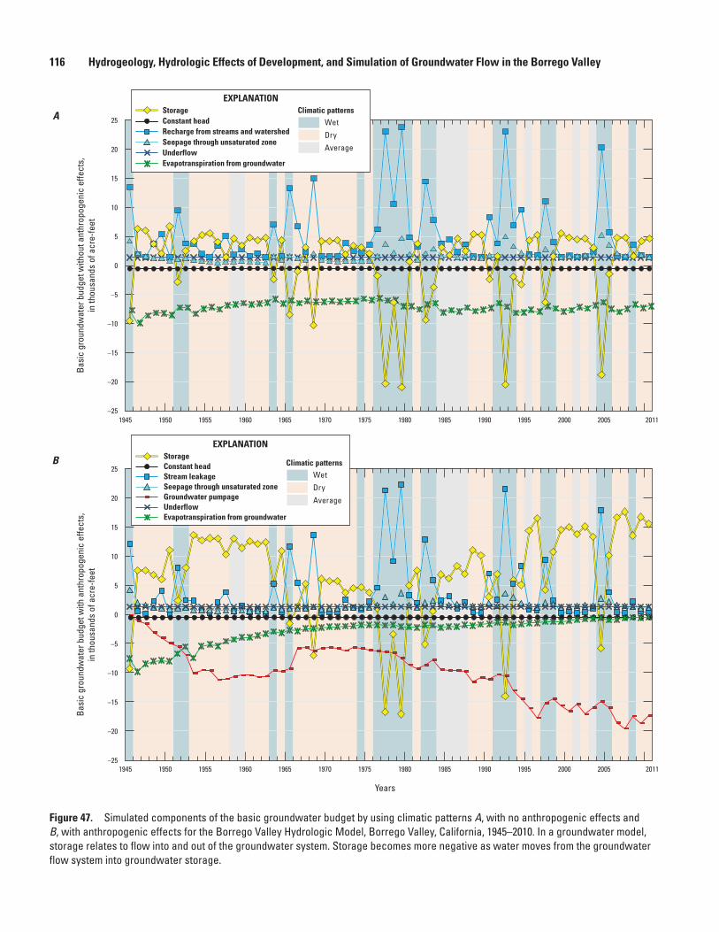
116 Hydrogeology, Hydrologic Effects of Development, and Simulation of Groundwater Flow in the Borrego Valley
sac13-0509_fig47ab
Fig. 47b. Major components of groundwater budgetFig. 47a Major components of groundwater budget
–25
–20
–15
–10
–5
0
5
10
15
20
25
1945 1955 1965 1975 1985 1995 2005
Years
B
1950 1960 1970 1980 1990 2000
–25
–20
–15
–10
–5
0
5
10
15
20
25
1945 19551950 1960 1970 1980 1990 20001965 1975 1985 1995 2005 2011
A
Basi
c gr
ound
wat
er b
udge
t with
out a
nthr
opog
enic
effe
cts,
in th
ousa
nds
of a
cre-
feet
2011
Constant headStream leakageSeepage through unsaturated zoneGroundwater pumpageUnderflow
EXPLANATION
Climatic patternsWet
Dry
Average
StorageConstant headRecharge from streams and watershedSeepage through unsaturated zone
Evapotranspiration from groundwater
Evapotranspiration from groundwater
EXPLANATIONClimatic patterns
Wet
Dry
AverageUnderflow
Storage
Basi
c gr
ound
wat
er b
udge
t with
ant
hrop
ogen
ic e
ffect
s,in
thou
sand
s of
acr
e-fe
et
Figure 47. Simulated components of the basic groundwater budget by using climatic patterns A, with no anthropogenic effects and B, with anthropogenic effects for the Borrego Valley Hydrologic Model, Borrego Valley, California, 1945–2010. In a groundwater model, storage relates to flow into and out of the groundwater system. Storage becomes more negative as water moves from the groundwater flow system into groundwater storage.
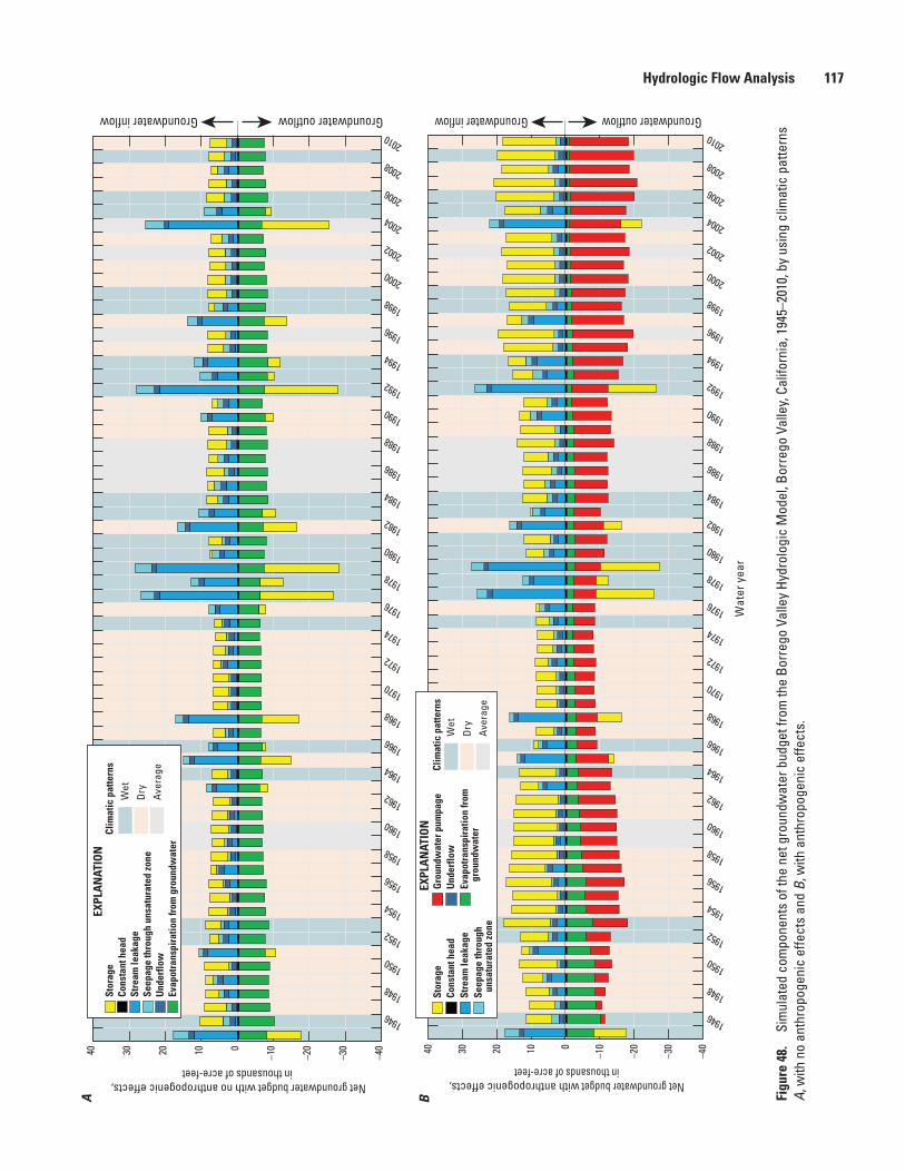
Hydrologic Flow Analysis 117
sac1
3-05
09_f
ig48
ab
Net
Gro
und-
Wat
er H
ydro
logi
c B
udge
t =>F
ig. 4
8b
Net
Gro
und-
Wat
er B
udge
t =>F
ig. 4
8a
Net groundwater budget with anthropogenic effects, in thousands of acre-feet
Groundwater inflow Groundwater outflow
–40
–30
–20
–10010203040
Net groundwater budget with no anthropogenic effects, in thousands of acre-feet
A
1946
1948
1950
1952
1954
1956
1958
1960
1962
1964
1966
1968
1970
1972
1974
1976
1978
1980
1982
1984
1986
1988
1990
1992
1994
1996
1998
2000
2002
2004
2006
2008
2010
–40
–30
–20
–10010203040
1946
1948
1950
1952
1954
1956
1958
1960
1962
1964
1966
1968
1970
1972
1974
1976
1978
1980
1982
1984
1986
1988
1990
1992
1994
1996
1998
2000
2002
2004
2006
2008
2010
Groundwater inflow Groundwater outflow
Wat
er y
ear
BSt
orag
eG
roun
dwat
er p
umpa
ge
Seep
age
thro
ugh
unsa
tura
ted
zone
Unde
rflo
wSt
ream
leak
age
Evap
otra
nspi
ratio
n fro
m
grou
ndw
ater
Cons
tant
hea
d
EXPL
AN
ATIO
NCl
imat
ic p
atte
rns
Wet
Dry
Ave
rage
EXPL
AN
ATIO
NSt
orag
e
Seep
age
thro
ugh
unsa
tura
ted
zone
Unde
rflo
w
Stre
am le
akag
e
Evap
otra
nspi
ratio
n fro
m g
roun
dwat
er
Cons
tant
hea
dCl
imat
ic p
atte
rns
Wet
Dry
Ave
rage
Figu
re 4
8.
Sim
ulat
ed c
ompo
nent
s of
the
net g
roun
dwat
er b
udge
t fro
m th
e Bo
rreg
o Va
lley
Hydr
olog
ic M
odel
, Bor
rego
Val
ley,
Cal
iforn
ia, 1
945–
2010
, by
usin
g cl
imat
ic p
atte
rns
A, w
ith n
o an
thro
poge
nic
effe
cts
and
B, w
ith a
nthr
opog
enic
effe
cts.
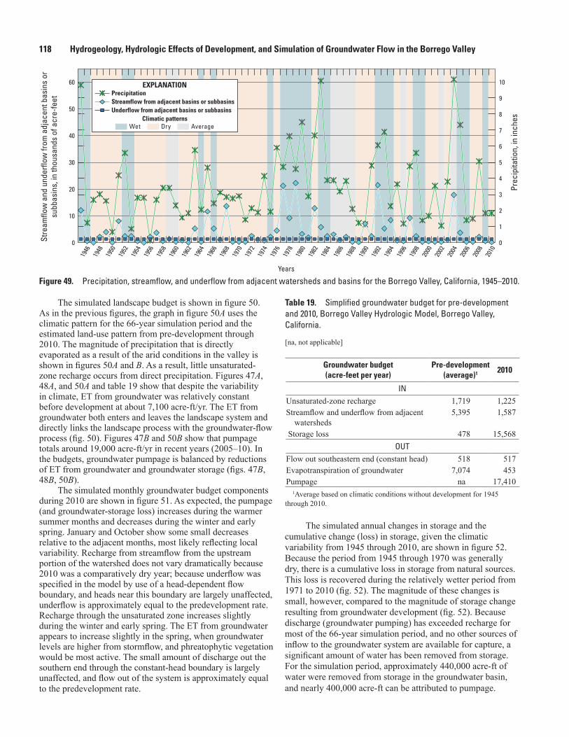
118 Hydrogeology, Hydrologic Effects of Development, and Simulation of Groundwater Flow in the Borrego Valley
Figure 49. Precipitation, streamflow, and underflow from adjacent watersheds and basins for the Borrego Valley, California, 1945–2010.
sac13-0509_fig49
Fig. 49 Precipitation in the basin and inflow from adjacent watersheds
0
10
Years
20
30
40
50
60
Stre
amflo
w a
nd u
nder
flow
from
adj
acen
t bas
ins
or
subb
asin
s, in
thou
sand
s of
acr
e-fe
et
0
1
2
3
4
5
6
7
8
9
10
Prec
ipita
tion,
in in
ches
PrecipitationStreamflow from adjacent basins or subbasinsUnderflow from adjacent basins or subbasins
EXPLANATION
Climatic patternsWet Dry Average
1946
1948
1950
1952
1954
1956
1958
1960
1962
1964
1966
1968
1970
1972
1974
1976
1978
1980
1982
1984
1986
1988
1990
1992
1994
1996
1998
2000
2002
2004
2006
2008
2010
The simulated landscape budget is shown in figure 50. As in the previous figures, the graph in figure 50A uses the climatic pattern for the 66-year simulation period and the estimated land-use pattern from pre-development through 2010. The magnitude of precipitation that is directly evaporated as a result of the arid conditions in the valley is shown in figures 50A and B. As a result, little unsaturated-zone recharge occurs from direct precipitation. Figures 47A, 48A, and 50A and table 19 show that despite the variability in climate, ET from groundwater was relatively constant before development at about 7,100 acre-ft/yr. The ET from groundwater both enters and leaves the landscape system and directly links the landscape process with the groundwater-flow process (fig. 50). Figures 47B and 50B show that pumpage totals around 19,000 acre-ft/yr in recent years (2005–10). In the budgets, groundwater pumpage is balanced by reductions of ET from groundwater and groundwater storage (figs. 47B, 48B, 50B).
The simulated monthly groundwater budget components during 2010 are shown in figure 51. As expected, the pumpage (and groundwater-storage loss) increases during the warmer summer months and decreases during the winter and early spring. January and October show some small decreases relative to the adjacent months, most likely reflecting local variability. Recharge from streamflow from the upstream portion of the watershed does not vary dramatically because 2010 was a comparatively dry year; because underflow was specified in the model by use of a head-dependent flow boundary, and heads near this boundary are largely unaffected, underflow is approximately equal to the predevelopment rate. Recharge through the unsaturated zone increases slightly during the winter and early spring. The ET from groundwater appears to increase slightly in the spring, when groundwater levels are higher from stormflow, and phreatophytic vegetation would be most active. The small amount of discharge out the southern end through the constant-head boundary is largely unaffected, and flow out of the system is approximately equal to the predevelopment rate.
The simulated annual changes in storage and the cumulative change (loss) in storage, given the climatic variability from 1945 through 2010, are shown in figure 52. Because the period from 1945 through 1970 was generally dry, there is a cumulative loss in storage from natural sources. This loss is recovered during the relatively wetter period from 1971 to 2010 (fig. 52). The magnitude of these changes is small, however, compared to the magnitude of storage change resulting from groundwater development (fig. 52). Because discharge (groundwater pumping) has exceeded recharge for most of the 66-year simulation period, and no other sources of inflow to the groundwater system are available for capture, a significant amount of water has been removed from storage. For the simulation period, approximately 440,000 acre-ft of water were removed from storage in the groundwater basin, and nearly 400,000 acre-ft can be attributed to pumpage.
Table 19. Simplified groundwater budget for pre-development and 2010, Borrego Valley Hydrologic Model, Borrego Valley, California.
[na, not applicable]
Groundwater budget (acre-feet per year)
Pre-development (average)1 2010
INUnsaturated-zone recharge 1,719 1,225 Streamflow and underflow from adjacent
watersheds 5,395 1,587
Storage loss 478 15,568 OUT
Flow out southeastern end (constant head) 518 517 Evapotranspiration of groundwater 7,074 453 Pumpage na 17,410
1Average based on climatic conditions without development for 1945 through 2010.
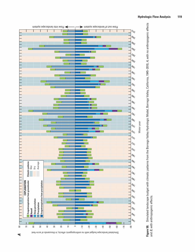
Hydrologic Flow Analysis 119
Figu
re 5
0.
Sim
ulat
ed la
ndsc
ape
budg
et w
ith c
limat
ic p
atte
rns
from
the
Borr
ego
Valle
y Hy
drol
ogic
Mod
el, B
orre
go V
alle
y, C
alifo
rnia
, 194
5–20
10, A
, with
no
anth
ropo
geni
c ef
fect
s an
d B,
with
ant
hrop
ogen
ic e
ffect
s.
sac1
3-05
09_f
ig50
a
Tota
l Lan
dsca
pe B
udge
t thr
ough
tim
e fo
r Bor
rego
Val
ley,
Cal
iforn
ia =
> Fi
g. 5
0a
–70
–80
–60
–50
–40
–30
–20
–1001020304050607080
Wat
er y
ear
Simulated landscape budget with no anthropogenic effects, in thousands of acre-feet
Flow into landscape system Flow out of landscape system
Evap
otra
nspi
ratio
n fro
m g
roun
dwat
erRu
noff
EXPL
AN
ATIO
N
Deep
per
cola
tion
Prec
ipita
tion
Evap
otra
nspi
ratio
n fro
m p
reci
pita
tion
Clim
atic
pat
tern
sW
et
Dry
Ave
rage
1946
1948
1950
1952
1954
1956
1958
1960
1962
1964
1966
1968
1970
1972
1974
1976
1978
1980
1982
1984
1986
1988
1990
1992
1994
1996
1998
2000
2002
2004
2006
2008
2010
A
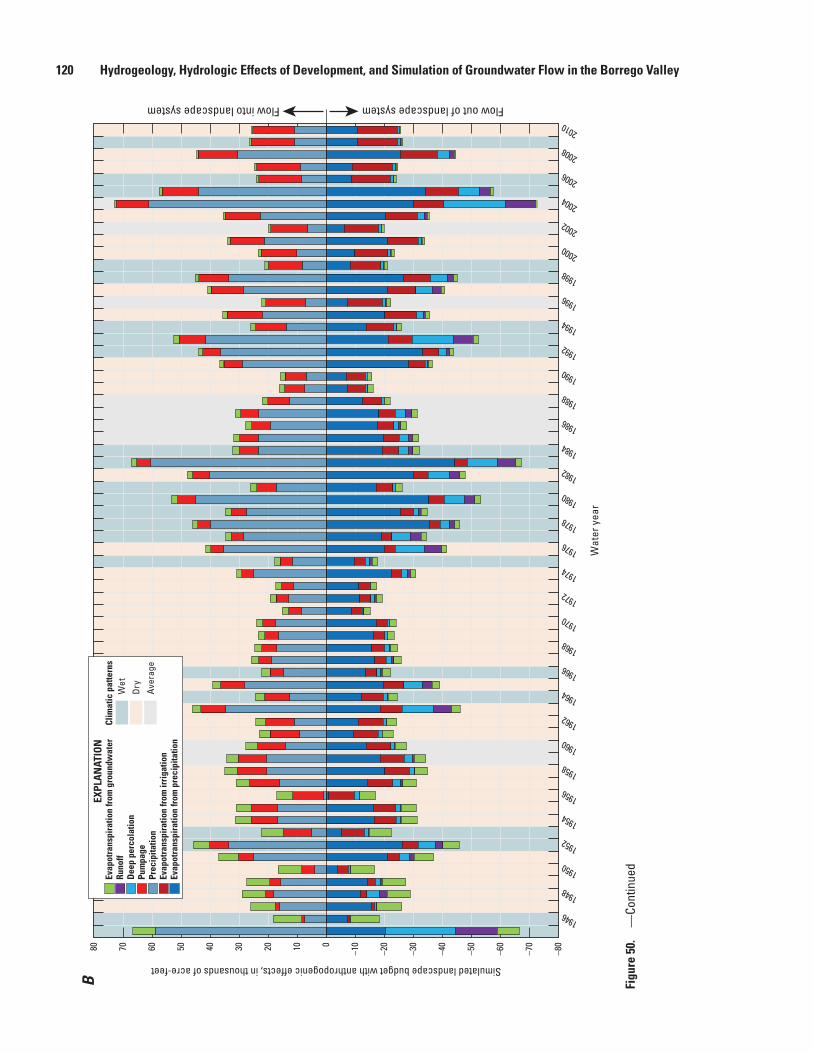
120 Hydrogeology, Hydrologic Effects of Development, and Simulation of Groundwater Flow in the Borrego Valley
Figu
re 5
0.
—Co
ntin
ued
sac1
3-05
09_f
ig50
b
–80
–70
–60
–50
–40
–30
–20
–1001020304050607080
Wat
er y
ear
Simulated landscape budget with anthropogenic effects, in thousands of acre-feet
Flow into landscape system Flow out of landscape system
Evap
otra
nspi
ratio
n fro
m g
roun
dwat
erRu
noff
EXPL
AN
ATIO
N
Deep
per
cola
tion
Pum
page
Prec
ipita
tion
Evap
otra
nspi
ratio
n fro
m ir
rigat
ion
Evap
otra
nspi
ratio
n fro
m p
reci
pita
tion
Clim
atic
pat
tern
sW
et
Dry
Ave
rage
1946
1948
1950
1952
1954
1956
1958
1960
1962
1964
1966
1968
1970
1972
1974
1976
1978
1980
1982
1984
1986
1988
1990
1992
1994
1996
1998
2000
2002
2004
2006
2008
2010
B
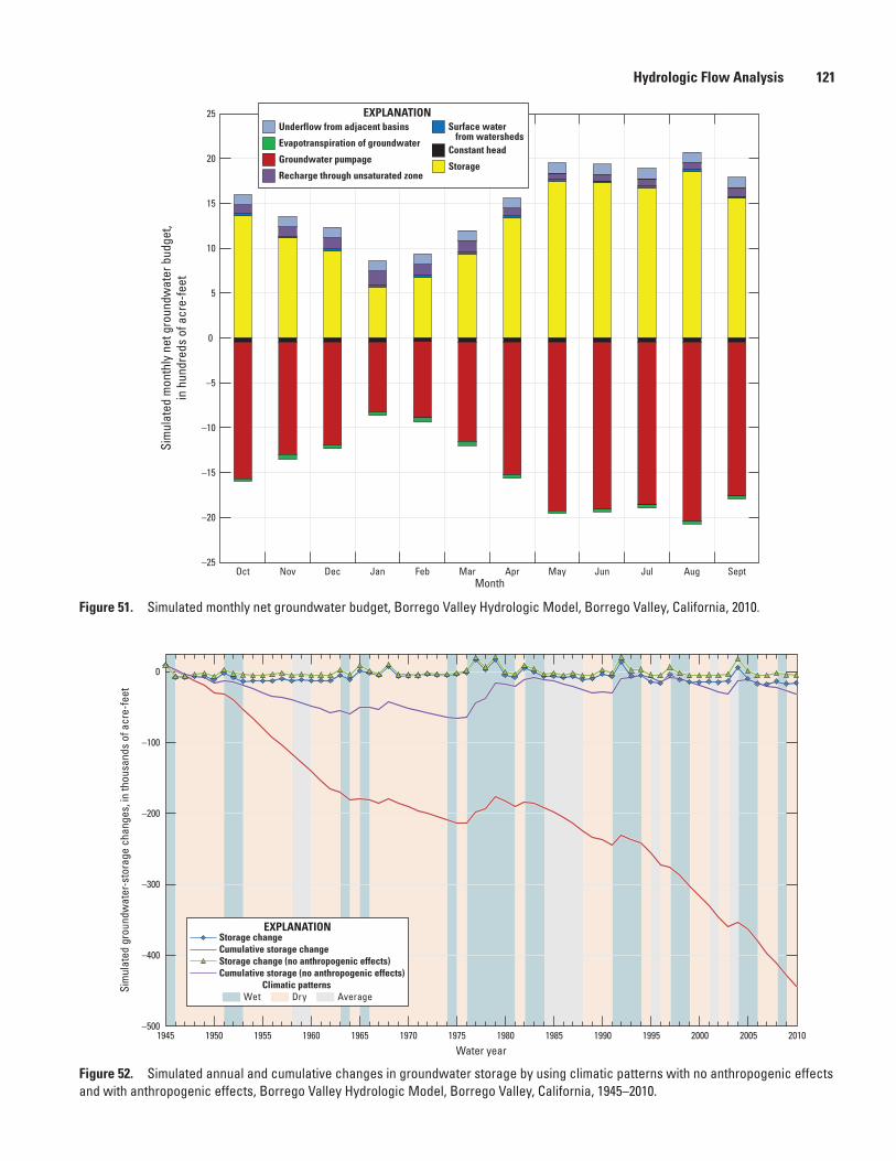
Hydrologic Flow Analysis 121
Figure 51. Simulated monthly net groundwater budget, Borrego Valley Hydrologic Model, Borrego Valley, California, 2010.
Figure 52. Simulated annual and cumulative changes in groundwater storage by using climatic patterns with no anthropogenic effects and with anthropogenic effects, Borrego Valley Hydrologic Model, Borrego Valley, California, 1945–2010.
sac13-0509_fig51
Water Year 2010 Net Groundwater budget fig. 51
–25
Month
–20
–15
–10
–5
0
5
10
15
20
25
Oct Nov Dec Jan Feb Mar Apr May Jun Jul Aug Sept
Underflow from adjacent basins
Evapotranspiration of groundwater
Groundwater pumpage
Recharge through unsaturated zone
Surface water from watersheds
Constant head
Storage
EXPLANATION
Sim
ulat
ed m
onth
ly n
et g
roun
dwat
er b
udge
t,in
hun
dred
s of
acr
e-fe
et
sac13-0509_fig52
Fig. 52 Storage changes
–500
–400
–300
–200
–100
0
Water year1945 1950 1955 1960 1965 1970 1975 1980 1985 1990 1995 2000 2005 2010
Sim
ulat
ed g
roun
dwat
er-s
tora
ge c
hang
es, i
n th
ousa
nds
of a
cre-
feet
Storage changeCumulative storage changeStorage change (no anthropogenic effects)Cumulative storage (no anthropogenic effects)
EXPLANATION
Climatic patternsWet Dry Average
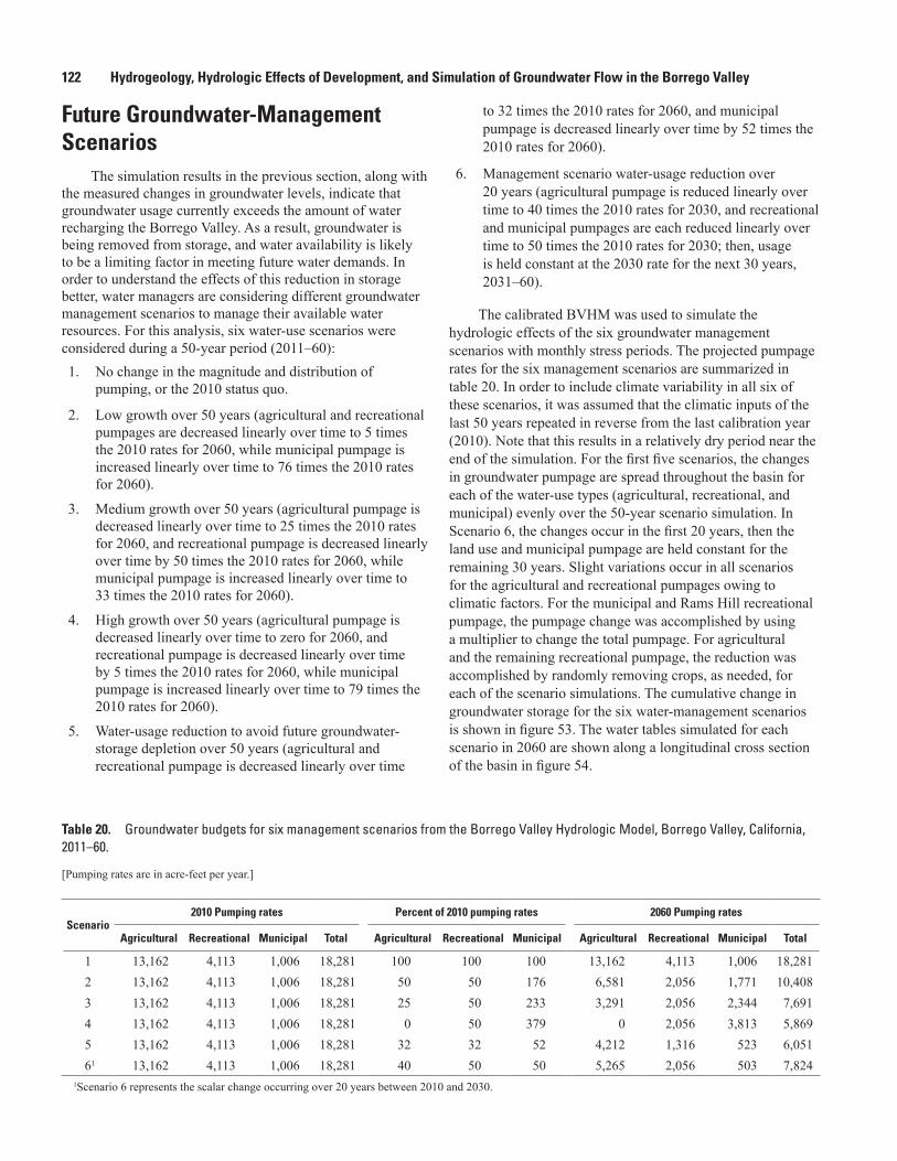
122 Hydrogeology, Hydrologic Effects of Development, and Simulation of Groundwater Flow in the Borrego Valley
Future Groundwater-Management Scenarios
The simulation results in the previous section, along with the measured changes in groundwater levels, indicate that groundwater usage currently exceeds the amount of water recharging the Borrego Valley. As a result, groundwater is being removed from storage, and water availability is likely to be a limiting factor in meeting future water demands. In order to understand the effects of this reduction in storage better, water managers are considering different groundwater management scenarios to manage their available water resources. For this analysis, six water-use scenarios were considered during a 50-year period (2011–60):1. No change in the magnitude and distribution of
pumping, or the 2010 status quo.
2. Low growth over 50 years (agricultural and recreational pumpages are decreased linearly over time to 5 times the 2010 rates for 2060, while municipal pumpage is increased linearly over time to 76 times the 2010 rates for 2060).
3. Medium growth over 50 years (agricultural pumpage is decreased linearly over time to 25 times the 2010 rates for 2060, and recreational pumpage is decreased linearly over time by 50 times the 2010 rates for 2060, while municipal pumpage is increased linearly over time to 33 times the 2010 rates for 2060).
4. High growth over 50 years (agricultural pumpage is decreased linearly over time to zero for 2060, and recreational pumpage is decreased linearly over time by 5 times the 2010 rates for 2060, while municipal pumpage is increased linearly over time to 79 times the 2010 rates for 2060).
5. Water-usage reduction to avoid future groundwater-storage depletion over 50 years (agricultural and recreational pumpage is decreased linearly over time
to 32 times the 2010 rates for 2060, and municipal pumpage is decreased linearly over time by 52 times the 2010 rates for 2060).
6. Management scenario water-usage reduction over 20 years (agricultural pumpage is reduced linearly over time to 40 times the 2010 rates for 2030, and recreational and municipal pumpages are each reduced linearly over time to 50 times the 2010 rates for 2030; then, usage is held constant at the 2030 rate for the next 30 years, 2031–60).
The calibrated BVHM was used to simulate the hydrologic effects of the six groundwater management scenarios with monthly stress periods. The projected pumpage rates for the six management scenarios are summarized in table 20. In order to include climate variability in all six of these scenarios, it was assumed that the climatic inputs of the last 50 years repeated in reverse from the last calibration year (2010). Note that this results in a relatively dry period near the end of the simulation. For the first five scenarios, the changes in groundwater pumpage are spread throughout the basin for each of the water-use types (agricultural, recreational, and municipal) evenly over the 50-year scenario simulation. In Scenario 6, the changes occur in the first 20 years, then the land use and municipal pumpage are held constant for the remaining 30 years. Slight variations occur in all scenarios for the agricultural and recreational pumpages owing to climatic factors. For the municipal and Rams Hill recreational pumpage, the pumpage change was accomplished by using a multiplier to change the total pumpage. For agricultural and the remaining recreational pumpage, the reduction was accomplished by randomly removing crops, as needed, for each of the scenario simulations. The cumulative change in groundwater storage for the six water-management scenarios is shown in figure 53. The water tables simulated for each scenario in 2060 are shown along a longitudinal cross section of the basin in figure 54.
Table 20. Groundwater budgets for six management scenarios from the Borrego Valley Hydrologic Model, Borrego Valley, California, 2011–60.
[Pumping rates are in acre-feet per year.]
Scenario2010 Pumping rates Percent of 2010 pumping rates 2060 Pumping rates
Agricultural Recreational Municipal Total Agricultural Recreational Municipal Agricultural Recreational Municipal Total
1 13,162 4,113 1,006 18,281 100 100 100 13,162 4,113 1,006 18,281 2 13,162 4,113 1,006 18,281 50 50 176 6,581 2,056 1,771 10,408 3 13,162 4,113 1,006 18,281 25 50 233 3,291 2,056 2,344 7,691 4 13,162 4,113 1,006 18,281 0 50 379 0 2,056 3,813 5,869 5 13,162 4,113 1,006 18,281 32 32 52 4,212 1,316 523 6,051 61 13,162 4,113 1,006 18,281 40 50 50 5,265 2,056 503 7,824
1Scenario 6 represents the scalar change occurring over 20 years between 2010 and 2030.
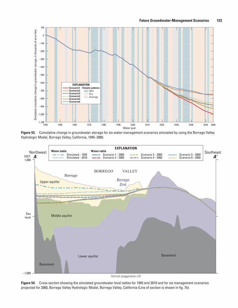
Future Groundwater-Management Scenarios 123
Figure 53. Cumulative change in groundwater storage for six water-management scenarios simulated by using the Borrego Valley Hydrologic Model, Borrego Valley, California, 1945–2060.
sac13-0509_fig53
Cumulative Storage change for water management scenarios
–1,100
–1,000
–800
–600
Sim
ulat
ed c
umul
ativ
e ch
ange
in g
roun
dwat
er s
tora
ge, i
n th
ouan
ds o
f acr
e-fe
et
–400
–200
0
100
–100
–300
–500
–700
–900
1945 1955 1965 1975 1985 1995 2005Water year
2015 2025 2035 2045 2055 2060
Scenario1Scenario2Scenario3Scenario4Scenario5Scenario6
EXPLANATIONClimatic patterns
WetDryAverage
–1,000
Sealevel
1,000A A’FEET
Vertical exaggeration ×10
EXPLANATION
Simulated - 1945 Simulated - 2010
Scenario 1 - 2060 Scenario 2 - 2060
Scenario 3 - 2060 Scenario 4 - 2060
Scenario 5 - 2060Scenario 6 - 2060
Water table Water table
sac13-0509_Figure 54_xsecs A_water levels
BORREGO VALLEYBorrego
Upper aquifer BorregoSink
Middle aquifer
Lower aquifer
Basement
Basement
Northwest Southeast
Figure 54. Cross section showing the simulated groundwater level tables for 1945 and 2010 and for six management scenarios projected for 2060, Borrego Valley Hydrologic Model, Borrego Valley, California (Line of section is shown in fig. 7b).
124 Hydrogeology, Hydrologic Effects of Development, and Simulation of Groundwater Flow in the Borrego Valley
Scenario 1: Status Quo
Scenario 1 consists of simulating the same stresses as the last calibration year (2010) for the 50-year horizon with no other management strategy. Although the simulated future pumpage is decreased for some years owing to climate variations, the future pumpage is still greater than simulated recharge for all years; consequently, the model simulation resulted in continued drawdowns and a large loss in storage (figs. 53, 55). Simulated drawdowns for 2011 through 2060 exceed 125 ft in the northern agriculturally dominated part of the valley, and groundwater levels decline to the middle aquifer in most of the basin as the upper aquifer drains.
Scenarios 2–4: Low, Medium, and High Municipal Growth Over 50 Years
Scenarios 2, 3, and 4, associated with low, medium, and high growth, respectively, involve reducing agricultural and recreational pumpages in various combinations, while linearly increasing municipal pumpage at different rates over 50 years. The low-growth scenario consists of an increase in municipal pumpage linearly to a maximum of 1.76 times 2010 rates until 2060 (table 20). The medium-growth scenario linearly increases municipal pumpage to 2.33 times the 2010 rates until 2060, and the high-growth scenario linearly increases municipal pumpage to 3.79 times the 2010 rates until 2060. Like the status quo Scenario 1, simulated future pumpage exceeds recharge rates in Scenarios 2 and 3. Therefore, each of these two scenarios increases the loss in storage and drawdowns. Simulated maximum water-level declines occurred in the southwestern part of the basin, particularly near the BWD supply wells. Because agricultural and recreational pumping continue in Scenarios 2 and 3, drawdown and storage losses continue in the areas where this pumping occurs. With the eventual removal of agricultural pumpage, Scenario 4 reaches a pumping rate that is less than the rate of recharge to the groundwater system at the end of the 50-year scenario.
Scenario 5: Water-Usage Reduction to Avoid Future Groundwater Storage Depletion Over 50 Years
In terms of water-resources management, ‘sustainable’ is a subjective term whose definition typically depends on various socio-economic, cultural, aesthetic factors in addition to physical-process factors, and thus, there are many ways to
define sustainability. In Scenario 5, sustainability is defined as groundwater recharge, on average, equaling groundwater discharge (over the long run there is no change in groundwater storage). In order to reach sustainability as defined, combined groundwater losses from ET, underflow, and pumping cannot exceed inflows from recharge and underflow. To accomplish this balance, agricultural and recreational pumpages were both reduced to 32 percent of current rates, and municipal pumpage was reduced to 52 percent of current rates (2010). These changes were applied linearly over 50 years. Simulated maximum water-level declines occur in the northern and western parts of the basin, where pumping is centered. Because agricultural, recreational, and municipal pumping continue, drawdown and storage losses continue in the areas where this pumping occurs. As total outflows (pumpage, ET, and underflow) approach the rate of total inflows (recharge and underflow), the cumulative change in storage approaches a constant value (slope approaches zero; fig. 53). Simulated drawdowns from 2011 through 2060 are approximately 60 ft in the northern, agriculturally dominated, part of the valley. Because pumpage rates are lower than for Scenario 1, the levels do not decline into the middle aquifer in most of the basin. The results for this scenario indicate that there would be small storage gains and losses that fluctuate with climatic variability. However, in the long run, the groundwater levels are relatively stable, although still much lower than pre-development conditions.
Scenario 6: Management Scenario for Rapid Changes Over 20 Years
In order to simulate what is thought to be realistic, but more rapid, changes during the next 20 years (2011–30), municipal and recreational pumpages both were reduced to 50 percent of current rates (2010), and agricultural pumpage was reduced to 40 percent of current rates by 2030 (table 20; fig. 53). These changes were applied linearly over 20 years. The 2030 pumpage rates were then held constant for the next 30 years to 2060. Simulated drawdowns from 2011 through 2060 were greater than 25 ft throughout much of the northern part of the basin. Because agricultural, recreational, and municipal pumping continue at rates greater than recharge, drawdown and storage losses continue in the areas where this pumping occurs (fig. 56). Because pumpage is lower than in Scenario 1, the levels do not decline to the middle aquifer in most of the basin. Although in the long run, groundwater levels would continue to decline, they would decline at slower rates than those simulated in Scenario 1, and storage gains and losses would fluctuate with climatic variability.
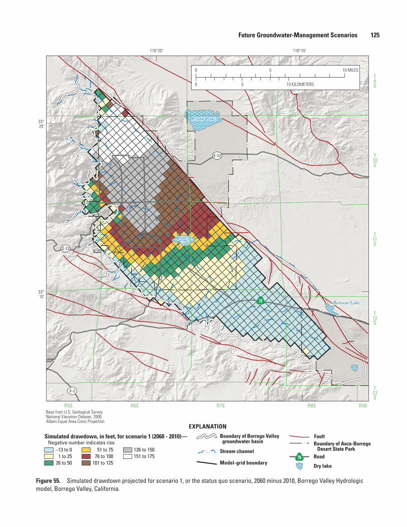
Future Groundwater-Management Scenarios 125
Figure 55. Simulated drawdown projected for scenario 1, or the status quo scenario, 2060 minus 2010, Borrego Valley Hydrologic model, Borrego Valley, California.
Clark Lake
BorregoSink
Benson Lake
T9S
T10S
T11S
T12S
T13S
R5E R6E R7E R8E R9EBase from U.S. Geological Survey National Elevation Dataset, 2006Albers Equal Area Conic Projection
S-22
S-22
S-2
78
116°10’116°20’
33°20’
33°10’
0
0 5 10
5 10 MILES
KILOMETERS
sac13-0509_Figure 55 drawdown_scen1
EXPLANATION
Simulated drawdown, in feet, for scenario 1 (2060 - 2010)— Negative number indicates rise
26 to 50
–13 to 01 to 25
101 to 125
51 to 7576 to 100
126 to 150151 to 175
Model-grid boundary
Stream channel
Boundary of Borrego Valley groundwater basin Boundary of Anza-Borrego
Desert State Park
Fault
Road78
Dry lake
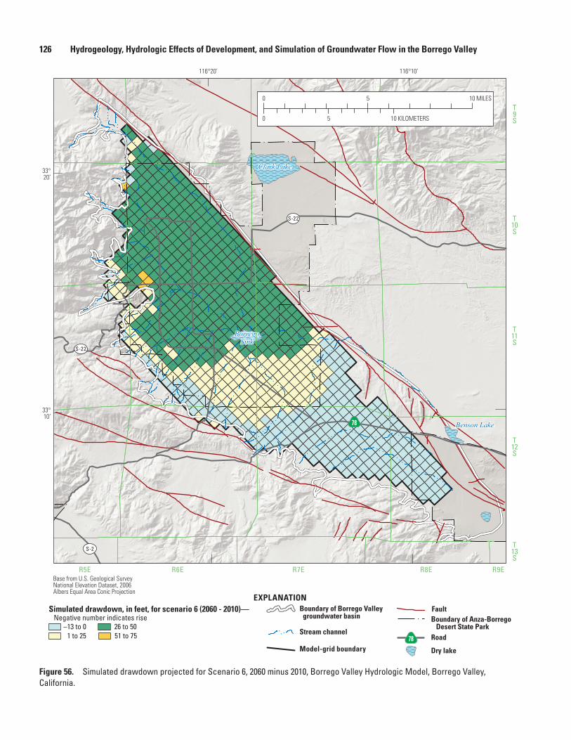
126 Hydrogeology, Hydrologic Effects of Development, and Simulation of Groundwater Flow in the Borrego Valley
Clark Lake
BorregoSink
Benson Lake
T9S
T10S
T11S
T12S
T13S
R5E R6E R7E R8E R9EBase from U.S. Geological Survey National Elevation Dataset, 2006Albers Equal Area Conic Projection
S-22
S-22
S-2
78
116°10’116°20’
33°20’
33°10’
0
0 5 10
5 10 MILES
KILOMETERS
sac13-0509_Figure 56 Sim drawdown_Scen6
EXPLANATIONSimulated drawdown, in feet, for scenario 6 (2060 - 2010)— Negative number indicates rise
–13 to 01 to 25
26 to 5051 to 75
Model-grid boundary
Stream channel
Boundary of Borrego Valley groundwater basin Boundary of Anza-Borrego
Desert State Park
Fault
Road78
Dry lake
Figure 56. Simulated drawdown projected for Scenario 6, 2060 minus 2010, Borrego Valley Hydrologic Model, Borrego Valley, California.
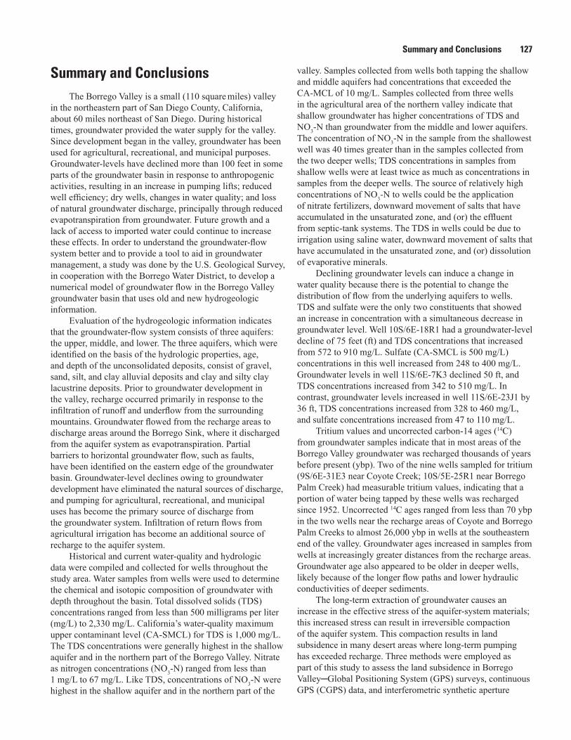
Summary and Conclusions 127
Summary and ConclusionsThe Borrego Valley is a small (110 square miles) valley
in the northeastern part of San Diego County, California, about 60 miles northeast of San Diego. During historical times, groundwater provided the water supply for the valley. Since development began in the valley, groundwater has been used for agricultural, recreational, and municipal purposes. Groundwater-levels have declined more than 100 feet in some parts of the groundwater basin in response to anthropogenic activities, resulting in an increase in pumping lifts; reduced well efficiency; dry wells, changes in water quality; and loss of natural groundwater discharge, principally through reduced evapotranspiration from groundwater. Future growth and a lack of access to imported water could continue to increase these effects. In order to understand the groundwater-flow system better and to provide a tool to aid in groundwater management, a study was done by the U.S. Geological Survey, in cooperation with the Borrego Water District, to develop a numerical model of groundwater flow in the Borrego Valley groundwater basin that uses old and new hydrogeologic information.
Evaluation of the hydrogeologic information indicates that the groundwater-flow system consists of three aquifers: the upper, middle, and lower. The three aquifers, which were identified on the basis of the hydrologic properties, age, and depth of the unconsolidated deposits, consist of gravel, sand, silt, and clay alluvial deposits and clay and silty clay lacustrine deposits. Prior to groundwater development in the valley, recharge occurred primarily in response to the infiltration of runoff and underflow from the surrounding mountains. Groundwater flowed from the recharge areas to discharge areas around the Borrego Sink, where it discharged from the aquifer system as evapotranspiration. Partial barriers to horizontal groundwater flow, such as faults, have been identified on the eastern edge of the groundwater basin. Groundwater-level declines owing to groundwater development have eliminated the natural sources of discharge, and pumping for agricultural, recreational, and municipal uses has become the primary source of discharge from the groundwater system. Infiltration of return flows from agricultural irrigation has become an additional source of recharge to the aquifer system.
Historical and current water-quality and hydrologic data were compiled and collected for wells throughout the study area. Water samples from wells were used to determine the chemical and isotopic composition of groundwater with depth throughout the basin. Total dissolved solids (TDS) concentrations ranged from less than 500 milligrams per liter (mg/L) to 2,330 mg/L. California’s water-quality maximum upper contaminant level (CA-SMCL) for TDS is 1,000 mg/L. The TDS concentrations were generally highest in the shallow aquifer and in the northern part of the Borrego Valley. Nitrate as nitrogen concentrations (NO3-N) ranged from less than 1 mg/L to 67 mg/L. Like TDS, concentrations of NO3-N were highest in the shallow aquifer and in the northern part of the
valley. Samples collected from wells both tapping the shallow and middle aquifers had concentrations that exceeded the CA-MCL of 10 mg/L. Samples collected from three wells in the agricultural area of the northern valley indicate that shallow groundwater has higher concentrations of TDS and NO3-N than groundwater from the middle and lower aquifers. The concentration of NO3-N in the sample from the shallowest well was 40 times greater than in the samples collected from the two deeper wells; TDS concentrations in samples from shallow wells were at least twice as much as concentrations in samples from the deeper wells. The source of relatively high concentrations of NO3-N to wells could be the application of nitrate fertilizers, downward movement of salts that have accumulated in the unsaturated zone, and (or) the effluent from septic-tank systems. The TDS in wells could be due to irrigation using saline water, downward movement of salts that have accumulated in the unsaturated zone, and (or) dissolution of evaporative minerals.
Declining groundwater levels can induce a change in water quality because there is the potential to change the distribution of flow from the underlying aquifers to wells. TDS and sulfate were the only two constituents that showed an increase in concentration with a simultaneous decrease in groundwater level. Well 10S/6E-18R1 had a groundwater-level decline of 75 feet (ft) and TDS concentrations that increased from 572 to 910 mg/L. Sulfate (CA-SMCL is 500 mg/L) concentrations in this well increased from 248 to 400 mg/L. Groundwater levels in well 11S/6E-7K3 declined 50 ft, and TDS concentrations increased from 342 to 510 mg/L. In contrast, groundwater levels increased in well 11S/6E-23J1 by 36 ft, TDS concentrations increased from 328 to 460 mg/L, and sulfate concentrations increased from 47 to 110 mg/L.
Tritium values and uncorrected carbon-14 ages (14C) from groundwater samples indicate that in most areas of the Borrego Valley groundwater was recharged thousands of years before present (ybp). Two of the nine wells sampled for tritium (9S/6E-31E3 near Coyote Creek; 10S/5E-25R1 near Borrego Palm Creek) had measurable tritium values, indicating that a portion of water being tapped by these wells was recharged since 1952. Uncorrected 14C ages ranged from less than 70 ybp in the two wells near the recharge areas of Coyote and Borrego Palm Creeks to almost 26,000 ybp in wells at the southeastern end of the valley. Groundwater ages increased in samples from wells at increasingly greater distances from the recharge areas. Groundwater age also appeared to be older in deeper wells, likely because of the longer flow paths and lower hydraulic conductivities of deeper sediments.
The long-term extraction of groundwater causes an increase in the effective stress of the aquifer-system materials; this increased stress can result in irreversible compaction of the aquifer system. This compaction results in land subsidence in many desert areas where long-term pumping has exceeded recharge. Three methods were employed as part of this study to assess the land subsidence in Borrego Valley─Global Positioning System (GPS) surveys, continuous GPS (CGPS) data, and interferometric synthetic aperture
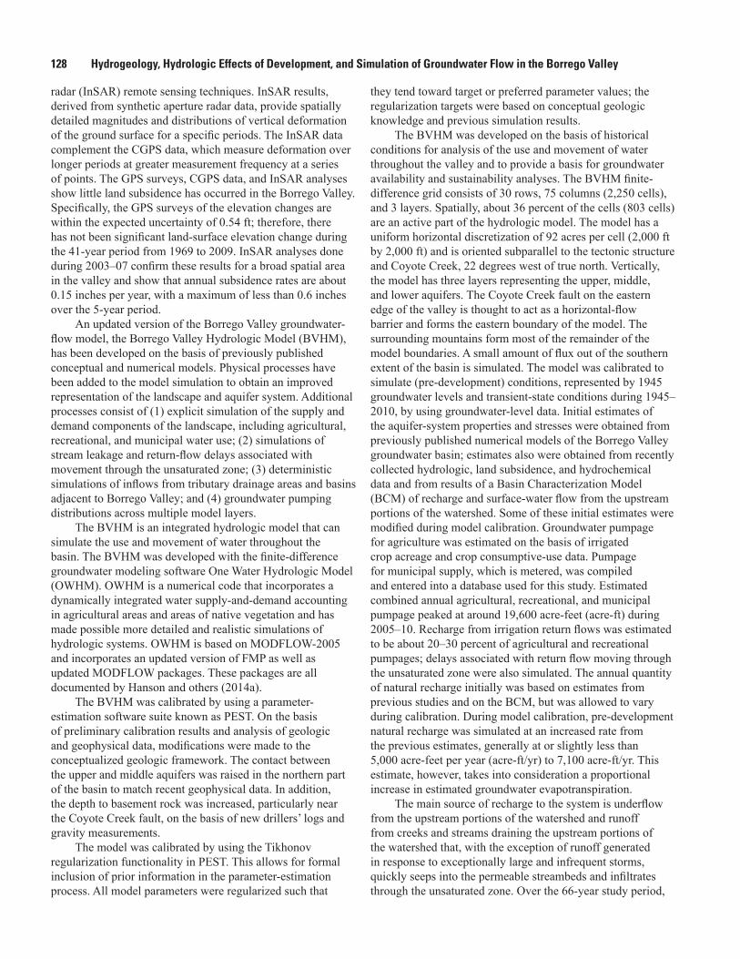
128 Hydrogeology, Hydrologic Effects of Development, and Simulation of Groundwater Flow in the Borrego Valley
radar (InSAR) remote sensing techniques. InSAR results, derived from synthetic aperture radar data, provide spatially detailed magnitudes and distributions of vertical deformation of the ground surface for a specific periods. The InSAR data complement the CGPS data, which measure deformation over longer periods at greater measurement frequency at a series of points. The GPS surveys, CGPS data, and InSAR analyses show little land subsidence has occurred in the Borrego Valley. Specifically, the GPS surveys of the elevation changes are within the expected uncertainty of 0.54 ft; therefore, there has not been significant land-surface elevation change during the 41-year period from 1969 to 2009. InSAR analyses done during 2003–07 confirm these results for a broad spatial area in the valley and show that annual subsidence rates are about 0.15 inches per year, with a maximum of less than 0.6 inches over the 5-year period.
An updated version of the Borrego Valley groundwater-flow model, the Borrego Valley Hydrologic Model (BVHM), has been developed on the basis of previously published conceptual and numerical models. Physical processes have been added to the model simulation to obtain an improved representation of the landscape and aquifer system. Additional processes consist of (1) explicit simulation of the supply and demand components of the landscape, including agricultural, recreational, and municipal water use; (2) simulations of stream leakage and return-flow delays associated with movement through the unsaturated zone; (3) deterministic simulations of inflows from tributary drainage areas and basins adjacent to Borrego Valley; and (4) groundwater pumping distributions across multiple model layers.
The BVHM is an integrated hydrologic model that can simulate the use and movement of water throughout the basin. The BVHM was developed with the finite-difference groundwater modeling software One Water Hydrologic Model (OWHM). OWHM is a numerical code that incorporates a dynamically integrated water supply-and-demand accounting in agricultural areas and areas of native vegetation and has made possible more detailed and realistic simulations of hydrologic systems. OWHM is based on MODFLOW-2005 and incorporates an updated version of FMP as well as updated MODFLOW packages. These packages are all documented by Hanson and others (2014a).
The BVHM was calibrated by using a parameter-estimation software suite known as PEST. On the basis of preliminary calibration results and analysis of geologic and geophysical data, modifications were made to the conceptualized geologic framework. The contact between the upper and middle aquifers was raised in the northern part of the basin to match recent geophysical data. In addition, the depth to basement rock was increased, particularly near the Coyote Creek fault, on the basis of new drillers’ logs and gravity measurements.
The model was calibrated by using the Tikhonov regularization functionality in PEST. This allows for formal inclusion of prior information in the parameter-estimation process. All model parameters were regularized such that
they tend toward target or preferred parameter values; the regularization targets were based on conceptual geologic knowledge and previous simulation results.
The BVHM was developed on the basis of historical conditions for analysis of the use and movement of water throughout the valley and to provide a basis for groundwater availability and sustainability analyses. The BVHM finite-difference grid consists of 30 rows, 75 columns (2,250 cells), and 3 layers. Spatially, about 36 percent of the cells (803 cells) are an active part of the hydrologic model. The model has a uniform horizontal discretization of 92 acres per cell (2,000 ft by 2,000 ft) and is oriented subparallel to the tectonic structure and Coyote Creek, 22 degrees west of true north. Vertically, the model has three layers representing the upper, middle, and lower aquifers. The Coyote Creek fault on the eastern edge of the valley is thought to act as a horizontal-flow barrier and forms the eastern boundary of the model. The surrounding mountains form most of the remainder of the model boundaries. A small amount of flux out of the southern extent of the basin is simulated. The model was calibrated to simulate (pre-development) conditions, represented by 1945 groundwater levels and transient-state conditions during 1945–2010, by using groundwater-level data. Initial estimates of the aquifer-system properties and stresses were obtained from previously published numerical models of the Borrego Valley groundwater basin; estimates also were obtained from recently collected hydrologic, land subsidence, and hydrochemical data and from results of a Basin Characterization Model (BCM) of recharge and surface-water flow from the upstream portions of the watershed. Some of these initial estimates were modified during model calibration. Groundwater pumpage for agriculture was estimated on the basis of irrigated crop acreage and crop consumptive-use data. Pumpage for municipal supply, which is metered, was compiled and entered into a database used for this study. Estimated combined annual agricultural, recreational, and municipal pumpage peaked at around 19,600 acre-feet (acre-ft) during 2005–10. Recharge from irrigation return flows was estimated to be about 20–30 percent of agricultural and recreational pumpages; delays associated with return flow moving through the unsaturated zone were also simulated. The annual quantity of natural recharge initially was based on estimates from previous studies and on the BCM, but was allowed to vary during calibration. During model calibration, pre-development natural recharge was simulated at an increased rate from the previous estimates, generally at or slightly less than 5,000 acre-feet per year (acre-ft/yr) to 7,100 acre-ft/yr. This estimate, however, takes into consideration a proportional increase in estimated groundwater evapotranspiration.
The main source of recharge to the system is underflow from the upstream portions of the watershed and runoff from creeks and streams draining the upstream portions of the watershed that, with the exception of runoff generated in response to exceptionally large and infrequent storms, quickly seeps into the permeable streambeds and infiltrates through the unsaturated zone. Over the 66-year study period,
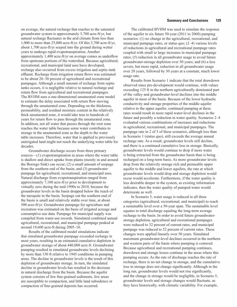
Summary and Conclusions 129
on average, the natural recharge that reaches to the saturated groundwater system is approximately 5,700 acre-ft/yr, but natural recharge fluctuates in the arid climate from less than 1,000 to more than 25,000 acre-ft/yr. Of this 5,700 acre-ft/yr, about 1,700 acre-ft/yr seeped into the ground during wetter years to undergo rapid evapotranspiration. Another approximately 1,400 acre-ft/yr on average comes as underflow from upstream portions of the watershed. Because agricultural, recreational, and municipal land uses have developed, recharge also occurred from excess irrigation and septic-tank effluent. Recharge from irrigation return flows was estimated to be about 20–30 percent of agricultural and recreational pumpages. Although a small amount of recharge from septic tanks occurs, it is negligible relative to natural recharge and return flow from agricultural and recreational pumpages. The BVHM uses a one-dimensional unsaturated-zone model to estimate the delay associated with return flow moving through the unsaturated zone. Depending on the thickness, permeability, and residual moisture content in the relatively thick unsaturated zone, it would take tens to hundreds of years for return flow to pass through the unsaturated zone. In addition, not all water that passes through the root zone reaches the water table because some water contributes to storage in the unsaturated zone as the depth to the water table increases. Therefore, water that is applied to previously unirrigated land might not reach the underlying water table for decades.
Groundwater discharge occurs from three primary sources—(1) evapotranspiration in areas where the water table is shallow and direct uptake from plants (mostly in and around the Borrego Sink) can occur; (2) a small amount of seepage from the southern end of the basin; and (3) groundwater pumpage for agricultural, recreational, and municipal uses. Natural discharge from evapotranspiration ranged from approximately 7,100 acre-ft/yr prior to development to virtually zero during the mid-1990s to 2010, because the groundwater levels in the basin dropped below the reach of the mesquite in the basin. Seepage out the southern end of the basin is small and relatively stable over time, at about 500 acre-ft/yr. Groundwater pumpage for agriculture and recreation was estimated on the basis of irrigated acreage and consumptive-use data. Pumpage for municipal supply was compiled from water-use records. Simulated combined annual agricultural, recreational, and municipal pumpage peaked at around 19,600 acre-ft during 2005–10.
Results of the calibrated model simulations indicate that simulated groundwater pumpage exceeded recharge in most years, resulting in an estimated cumulative depletion in groundwater storage of about 440,000 acre-ft. Groundwater pumping resulted in simulated groundwater levels declining by more than 150 ft relative to 1945 conditions in pumping areas. The decline in groundwater levels is the result of this depletion of groundwater storage. In turn, the simulated decline in groundwater levels has resulted in the decrease in natural discharge from the basin. Because the aquifer system consists of few fine-grained sediments, few areas are susceptible to compaction, and little land subsidence or compaction of fine-grained deposits has occurred.
The calibrated BVHM was used to simulate the response of the aquifer to six future 50-year (2011 to 2060) pumping scenarios: (1) no change in the agricultural, recreational, and municipal pumpage rates, or status quo; (2–4) various levels of reductions in agricultural and recreational pumpage rates coupled with small to large increases in municipal pumpage rates; (5) reduction in all groundwater usage to avoid future groundwater-storage depletion over 50 years; and (6) a less severe, but more rapid, reduction in all groundwater usage over 20 years, followed by 30 years at a constant, much lower usage rate.
Results from Scenario 1 indicate that the total drawdown observed since pre-development would continue, with values exceeding 125 ft in the northern agriculturally dominated part of the valley and groundwater-level declines into the middle aquifer in most of the basin. Because of the lower hydraulic conductivity and storage properties of the middle aquifer relative to the upper aquifer, continued pumping at these rates would result in more rapid water-level declines in the future and possibly a reduction in water quality. Scenarios 2–4 evaluated various combinations of increases and reductions in agricultural, recreational, and municipal pumpages. The pumpage rate in 2 of 3 of these scenarios, although less than in Scenario 1 (status quo), still exceeds the average annual recharge rate. As a result, groundwater levels still decline, and there is a continued cumulative loss in storage. Basically, groundwater levels would continue to drop if more water is being extracted from the groundwater basin than is being recharged on a long-term basis. As more groundwater levels drop from the relatively storage rich and permeable upper aquifer to the middle and lower aquifers, the rate at which groundwater levels would drop and storage depletion would occur would accelerate. Furthermore, if the water quality is less desirable deeper in the system, as existing information indicates, then the water quality of pumped water would deteriorate as well.
In Scenario 5, water usage is reduced in all three categories (agricultural, recreational, and municipal) to reach a sustainable level over a 50-year span. The sustainable level equates to total discharge equaling the long-term average recharge to the basin. In order to avoid future groundwater-storage depletion, agricultural and recreational pumpages were reduced to 32 percent of current rates, and municipal pumpage was reduced to 52 percent of current rates. These changes were applied linearly over 50 years. Simulated maximum groundwater-level declines occurred in the northern and western parts of the basin where pumping is centered. Because agricultural and recreational pumping continues, drawdown and storage losses continue in the areas where this pumping occurs. As the rate of discharge reaches the rate of recharge, there is no net change in storage, and the cumulative loss in storage does not change significantly. Although in the long run, groundwater levels would not rise significantly, and the change in storage would be negligible, in Scenario 5, groundwater levels and storage changes would fluctuate, as they have historically, with climatic variability. For example,
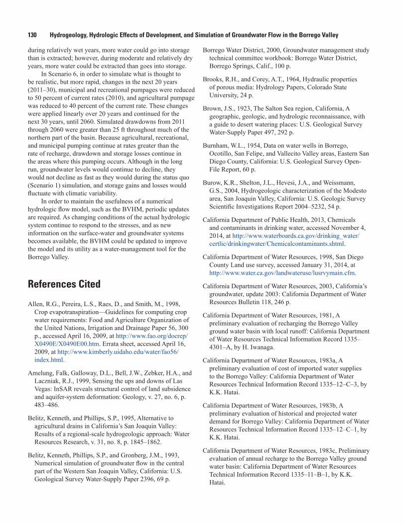
130 Hydrogeology, Hydrologic Effects of Development, and Simulation of Groundwater Flow in the Borrego Valley
during relatively wet years, more water could go into storage than is extracted; however, during moderate and relatively dry years, more water could be extracted than goes into storage.
In Scenario 6, in order to simulate what is thought to be realistic, but more rapid, changes in the next 20 years (2011–30), municipal and recreational pumpages were reduced to 50 percent of current rates (2010), and agricultural pumpage was reduced to 40 percent of the current rate. These changes were applied linearly over 20 years and continued for the next 30 years, until 2060. Simulated drawdowns from 2011 through 2060 were greater than 25 ft throughout much of the northern part of the basin. Because agricultural, recreational, and municipal pumping continue at rates greater than the rate of recharge, drawdown and storage losses continue in the areas where this pumping occurs. Although in the long run, groundwater levels would continue to decline, they would not decline as fast as they would during the status quo (Scenario 1) simulation, and storage gains and losses would fluctuate with climatic variability.
In order to maintain the usefulness of a numerical hydrologic flow model, such as the BVHM, periodic updates are required. As changing conditions of the actual hydrologic system continue to respond to the stresses, and as new information on the surface-water and groundwater systems becomes available, the BVHM could be updated to improve the model and its utility as a water-management tool for the Borrego Valley.
References Cited
Allen, R.G., Pereira, L.S., Raes, D., and Smith, M., 1998, Crop evapotranspiration—Guidelines for computing crop water requirements: Food and Agriculture Organization of the United Nations, Irrigation and Drainage Paper 56, 300 p., accessed April 16, 2009, at http://www.fao.org/docrep/X0490E/X0490E00.htm. Errata sheet, accessed April 16, 2009, at http://www.kimberly.uidaho.edu/water/fao56/index.html.
Amelung, Falk, Galloway, D.L., Bell, J.W., Zebker, H.A., and Laczniak, R.J., 1999, Sensing the ups and downs of Las Vegas: InSAR reveals structural control of land subsidence and aquifer-system deformation: Geology, v. 27, no. 6, p. 483–486.
Belitz, Kenneth, and Phillips, S.P., 1995, Alternative to agricultural drains in California’s San Joaquin Valley: Results of a regional-scale hydrogeologic approach: Water Resources Research, v. 31, no. 8, p. 1845–1862.
Belitz, Kenneth, Phillips, S.P., and Gronberg, J.M., 1993, Numerical simulation of groundwater flow in the central part of the Western San Joaquin Valley, California: U.S. Geological Survey Water-Supply Paper 2396, 69 p.
Borrego Water District, 2000, Groundwater management study technical committee workbook: Borrego Water District, Borrego Springs, Calif., 100 p.
Brooks, R.H., and Corey, A.T., 1964, Hydraulic properties of porous media: Hydrology Papers, Colorado State University, 24 p.
Brown, J.S., 1923, The Salton Sea region, California, A geographic, geologic, and hydrologic reconnaissance, with a guide to desert watering places: U.S. Geological Survey Water-Supply Paper 497, 292 p.
Burnham, W.L., 1954, Data on water wells in Borrego, Ocotillo, San Felipe, and Vallecito Valley areas, Eastern San Diego County, California: U.S. Geological Survey Open-File Report, 60 p.
Burow, K.R., Shelton, J.L., Hevesi, J.A., and Weissmann, G.S., 2004, Hydrogeologic characterization of the Modesto area, San Joaquin Valley, California: U.S. Geologic Survey Scientific Investigations Report 2004–5232, 54 p.
California Department of Public Health, 2013, Chemicals and contaminants in drinking water, accessed November 4, 2014, at http://www.waterboards.ca.gov/drinking_water/certlic/drinkingwater/Chemicalcontaminants.shtml.
California Department of Water Resources, 1998, San Diego County Land use survey, accessed January 31, 2014, at http://www.water.ca.gov/landwateruse/lusrvymain.cfm.
California Department of Water Resources, 2003, California’s groundwater, update 2003: California Department of Water Resources Bulletin 118, 246 p.
California Department of Water Resources, 1981, A preliminary evaluation of recharging the Borrego Valley ground water basin with local runoff: California Department of Water Resources Technical Information Record 1335–4301–A, by H. Iwanaga.
California Department of Water Resources, 1983a, A preliminary evaluation of cost of imported water supplies to the Borrego Valley: California Department of Water Resources Technical Information Record 1335–12–C–3, by K.K. Hatai.
California Department of Water Resources, 1983b, A preliminary evaluation of historical and projected water demand for Borrego Valley: California Department of Water Resources Technical Information Record 1335–12–C–1, by K.K. Hatai.
California Department of Water Resources, 1983c, Preliminary evaluation of annual recharge to the Borrego Valley ground water basin: California Department of Water Resources Technical Information Record 1335–11–B–1, by K.K. Hatai.
References Cited 131
California Department of Water Resources, 1984a, Borrego Valley water management plan: California Department of Water Resources 45 p.
California Department of Water Resources, 1984b, Evaluation of future operations of the Borrego Valley ground water basin: California Department of Water Resources Technical Information Record 1335–11–B–2, by P. Louie and H. Iwanaga.
California Department of Water Resources, 2015, California Sustainable Groundwater Management Act, accessed July 3, 2015, http://www.water.ca.gov/cagroundwater/moresgma.cfm.
California Irrigation Management System, 2012, California ETo zones map: California Department of Water Resources, accessed January 15, 2014, http://wwwcimis.water.ca.gov/App_Themes/images/etozonemap.jpg.
Clark, I.D., and Fritz, P., 1997, Environmental isotopes in hydrogeology: New York, Lewis Publishers, 328 p.
Craig, H., and Lal, D., 1961, The production rate of natural tritium: Tellus, v. 13, no. 1, p. 85–105.
Daly, C., Gibson, W.P., Doggett, M., Smith, J., and Taylor, G., 2004, Up-to-date monthly climate maps for the conterminous United States, in Proceedings of the 14th American Meteorological Society Conference on applied climatology, January 13–16, 2004: Seattle, Wash., American Meteorological Society, Paper P5.1, CD-ROM.
Dibblee, T.W., Jr., 1954, Geology of the Imperial Valley region, in Jahns, R.H., ed., Geology of southern California: California Division of Mines Bulletin 170, chap. 2, p. 21–28.
Dibblee, T.W., Jr., 1984, Stratigraphy and tectonics of the San Felipe Hills, Borrego Badlands, Superstition Hills, and vicinity, in Rigsby, C.A., ed., The Imperial Basin—Tectonics, Sediments, and Thermal Aspects: Pacific Section SEPM, p. 31–34.
Dimitrakopoulos, Roussos, and Desbarats, A.J., 1993, Geostatistical modeling of grid block permeabilities for 3D reservoir simulators: Reservoir Engineering, v. 8, p. 13–18.
Doherty, J.E., 2003, Groundwater model calibration using pilot points and regularization: Ground Water, v. 41, no. 2, p. 170–177, doi:10.1111/j.17456584.2003.tb02580.x.
Doherty, J., 2010a, PEST, Model-independent parameter estimation—User manual (5th ed., with slight additions): Brisbane, Australia, Watermark Numerical Computing.
Doherty, J., 2010b, Addendum to the PEST manual: Brisbane, Australia, Watermark Numerical Computing.
Doherty, J., 2010c, BeoPEST for Windows: Brisbane, Australia, Watermark Numerical Computing.
Doherty, J.E., and Hunt, R.J., 2010, Approaches to highly parameterized inversion—A guide to using PEST for groundwater-model calibration: U.S. Geological Survey Scientific Investigations Report 2010–5169, 59 p.
Dorsey, R.J., 2002, Stratigraphic record of Pleistocene initiation and slip on the Coyote Creek fault, Lower Coyote Creek, southern California, in Barth A., ed., Contributions to crustal evolution of the Southwestern United States: Boulder, Colorado, Geological Society of America Special Paper 365, p. 251–269.
Faunt, C.C., Hanson R.T., Schmid, Wolfgang, Belitz, K., and Predmore, S., 2009a, Documentation of the Ground-water Flow Model: U.S. Geological Survey Professional Paper 1766, Chapter C of Ground-Water Availability of California’s Central Valley, Claudia Faunt, ed., p. 121–212
Faunt, C.C., Belitz, K., and Hanson, R.T., 2009b, Texture Model of the valley fill deposits of the Central Valley, California: Hydrogeology Journal, DOI 10.1007/s10040–009–0539–7, 25 p.
Fielding, E.J., Blom, R.G., and Goldstein, R.M., 1998, Rapid subsidence over oil fields measured by SAR interferometry: Geophysical Research Letters, v. 27, p. 3215–3218.
Fio, J.L., and Leighton, D.A., 1995, Hydrogeologic framework, historical development of the ground-water system, and general hydrologic and water-quality conditions in 1990, South San Francisco Bay and Peninsula area, California: U.S. Geological Survey Open-File Report 94–357, 46 p.
Flint, A.L, and Flint, L.E., 2007a, Application of the Basin Characterization Model to estimate in-place recharge and runoff potential in the Basin and Range carbonate-rock aquifer system, White Pine County, Nevada, and adjacent areas in Nevada and Utah: U.S. Geological Survey Scientific Investigations Report 2007–5099, 19 p., http://pubs.water.usgs.gov/sir20075099.
Flint, L.E., and Flint, A.L., 2007b, Regional analysis of groundwater recharge, in Stonestrom, D.A., Constantz, Jim, Ferre, T.P.A., and Leake, S.A., eds., Groundwater recharge in the arid and semiarid southwestern United States: U.S. Geological Survey Professional Paper 1703–B, p. 29–60, http://pubs.usgs.gov/pp/pp1703/b/.
Flint, L.E., and Martin, Peter, eds., with contributions by Brandt, Justin, Christensen, A.H., Flint, A.L., Flint, L.E., Hevesi, J.A., Jachens, Robert, Kulongoski, J.T., Martin, Peter, and Sneed, Michelle, 2012, Geohydrology of Big Bear Valley, California: Phase 1—Geologic framework, recharge, and preliminary assessment of the source and age of groundwater: U.S. Geological Survey Scientific Investigations Report 2012–5100, 112 p.
132 Hydrogeology, Hydrologic Effects of Development, and Simulation of Groundwater Flow in the Borrego Valley
Flint, A.L., Flint, L.E., Hevesi, J.A., and Blainey, J.M., 2004, Fundamental concepts of recharge in the Desert Southwest, a regional modeling perspective, in Hogan, J.F., Phillips, F.M., and Scanlon, B.R., eds., Groundwater recharge in a desert environment, the Southwestern United States: American Geophysical Union, Water Science and Applications Series, v. 9, p. 159–184.
Flint, A.L., Flint, L.E., and Masbruch, M.D., 2011, Input, calibration, uncertainty, and limitations of the Basin Characterization Model, Appendix 3 of Heilweil, V.M., and Brooks, L.E., eds., Conceptual Model of the great Basin Carbonate and Alluvial Aquifer System: U.S. Geological Survey Scientific Investigations Report 2010–5193, p. 149–163.
Flint, L.E., Flint, A.L., Stolp, B.J., and Danskin, W.R., 2012, A basin-scale approach for assessing water resources in a semiarid environment: San Diego region, California and Mexico: Hydrology and Earth System Sciences, v. 16, p. 1–17.
Flint, L.E., Flint, A.L., Thorne, J.H., and Boynton, R., 2013, Fine-scale hydrological modeling for climate change applications; using watershed calibrations to assess model performance for landscape projections: Ecological Processes, v. 2, no. 25, 21 p.
Folk, R.L., 1954, The distinction between grain size and mineral composition in sedimentary rock nomenclature: Journal of Geology, v. 62, no. 4, p. 344–359.
Fontes, J.C., and Garnier, J.M., 1979, Determination of the initial 14C activity of the total dissolved carbon: A review of the existing models and a new approach: Water Resources Research, v. 15, no. 2, p. 399–413.
Freeze, A.R., and Cherry, J.A., 1979, Groundwater: Englewood Cliffs, N.J., Prentice-Hall, Inc., 604 p.
Galloway, D.L., Hudnut, K.W., Ingebritsen, S.E., Phillips, S.P., Peltzer,G., Rogez, F., and Rosen, P.A., 1998, Detection of aquifer system compaction and land subsidence using interferometric synthetic aperture radar, Antelope Valley, Mojave Desert, California: Water Resources Research, v. 34, no. 10, p. 2573–2585.
Galloway, D.L., Jones, D.R., and Ingebritsen, S.E., eds., 1999, Land subsidence in the United States: U.S. Geological Survey Circular 1182, 177 p., http://pubs.usgs.gov/circ/circ1182/, accessed Sept. 21, 2015.
Halford, K.J., 2009, AnalyzeHOLE—An integrated wellbore flow analysis tool. U.S. Geological Survey Techniques and Methods 4-F2, 46 p.
Hanson, R.T., and Leake, S.A., 1998, Documentation for HYDMOD, A program for time-series data from the U.S. Geological Survey’s modular three-dimensional finite-difference ground-water flow model: U.S. Geological Survey Water-Resources Investigations Report 98–564, 57 p.
Hanson, R.T., Boyce, S.E., Schmid, Wolfgang, Hughes, J.D., Mehl, S.M., Leake, S.A., Maddock, Thomas, III, and Niswonger, R.G., 2014a, One-Water Hydrologic Flow Model (MODFLOW-OWHM): U.S. Geological Survey Techniques and Methods 6–A51, 120 p., http://dx.doi.org/10.3133/tm6A51.
Hanson, R.T., Flint, L.E., Faunt, C.C., Gibbs, D.R., and Schmid, W., 2014b, Hydrologic models and analysis of water availability in Cuyama Valley, California: U.S. Geological Survey Scientific Investigations Report 2014–5150, 150 p., http://dx.doi.org/10.3133/sir20145150.
Harbaugh, A.W., 2005, MODFLOW-2005, The U.S. Geological Survey modular groundwater model—The groundwater flow process: U.S. Geological Survey Techniques and Methods, book 6, chap. A16, [variously paged].
Harbaugh, A.W., Banta, E.R., Hill, M.C., and McDonald, M.G., 2000, MODFLOW-2000, The U.S. Geological Survey modular groundwater model—User guide to modularization concepts and the groundwater flow process: U.S. Geological Survey Open-File Report 00–92, 121 p.
Henderson, T.W., 2001, Hydrogeology and numerical modeling of the Borrego Valley aquifer system: Master’s Thesis, San Diego State University, 260 p.
Hill, M.C., and Tiedeman, C.R., 2007, Effective groundwater model calibration: with analysis of data, sensitivities, predictions, and uncertainty: New York, Wiley and Sons, 464 p.
Hill, M.C., Banta, E.R, Harbaugh, A.W., and Anderman, E.R., 2000, MODFLOW-2000, The U.S Geological Survey modular ground-water model—User guide to the observation, sensitivity, and parameter-estimation processes and three post-processing programs: U.S. Geological Survey Open-File Report 00–184, 209 p.
Hoffmann, J., Zebker, H.A., Galloway, D.L., and Amelung, F., 2001, Seasonal subsidence and rebound in Las Vegas Valley, Nevada, observed by synthetic aperture radar interferometry: Water Resources Research, v. 37, no. 6, p. 1551–1566.
Hogan, C.M., 2009, California Fan Palm: Washingtonia filifera, in Stromberg, Nicklas, ed., GlobalTwitcher.com.
References Cited 133
Hsieh, P.A., and Freckleton, J.R, 1993, Documentation of a computer program to simulate horizontal-flow barriers using the U.S. Geological Survey’s modular three-dimensional finite-difference ground-water from model: U.S. Geological Survey Open-File report 92–477, 32 p.
Hunt, C.B., 1967, Physiography of the United States: San Francisco and London, W.H. Freeman and Co., 480 p.
Hunt, R.J., Doherty, J., and Tonkin, M.J., 2007, Are models too simple? Arguments for increased parameterization: Issue Paper in Ground Water, v. 45, no. 3, p. 254–261. doi:10.1111/j.1745-6584.2007.00316.x.
Ikehara, M.E., Predmore, S.K., Swope, D.J., 1997, Geodetic network to evaluate historical elevation changes and to monitor land subsidence in lower Coachella Valley, California, 1996: U.S. Geological Survey Water-Resources Investigations Report, 97–4237, scale 1:63,000, 1 sheet.
Isaaks, E. H., and Srivastava, R. M., 1989, An introduction to applied geostatistics: New York, Oxford University Press, 561 p.
Izbicki, J.A., 2004, A small-diameter sample pump for collection of depth-dependent samples from production wells under pumping conditions: U.S. Geological Survey Fact Sheet 2004–3096, 2 p.
Izbicki, J.A., Christensen, A.H., and Hanson, R.T., 1999, U.S. Geological Survey combined well-bore flow and depth-dependent water sampler: U.S. Geological Survey Fact Sheet, FS–196–99.
Izbicki, J. A., Radyk, John, and Michel, R. L., 2002, Movement of water through a thick unsaturated zone underlying Oro Grande and Sheep Creek Washes in the western Mojave Desert, USA: Hydrogeology Journal, v. 10, no. 3, p. 409–427.
Journel, A.G., and Huijbregts, C.J., 1978, Mining geostatistics: New York, Academic Press, 600 p.
Konikow, L.F., Hornberger, G.Z., Halford, K.J., and Hanson, R.T., 2009, Revised multi-node well (MNW2) package for MODFLOW ground-water flow model: U.S. Geological Survey Techniques and Methods 6–A30, 67 p.
Koterba, M.T., Wilde, F.D., and Lapham, W.W., 1995, Groundwater data-collection protocols and procedures for the National Water-Quality Assessment Program—Collection and documentation of water-quality samples and related data: U.S. Geological Survey Open-File Report 95–399, 113 p.
Lane, E. W., 1947, Report of the subcommittee on sediment terminology: American Geophysical Union Transactions, v. 28, no. 6, p. 936–938.
Laudon, J., and Belitz, Kenneth, 1991, Texture and depositional history of late Pleistocene-Holocene alluvium in the central part of the western San Joaquin Valley, California: Bulletin of the Association of Engineering Geologists, v. 28, no. 1, p. 73–88.
Leake, S.A., and Lilly, M.R., 1997, Documentation of a computer program (FHB1) for assignment of transient specified-flow and specified-head boundaries in applications of the modular finite-difference ground-water flow model (MODFLOW): U.S. Geological Survey Open-File Report 97–571, 50 p.
Leighton, D.A., Fio, J.L., and Metzger, L.F., 1994, Database of well and areal data, South San Francisco Bay and Peninsula area, California: U.S. Geological Survey Water-Resources Investigations Report 94–4151, 47 p.
Loetlz, O.J., Irelan, Burge, Robison, J. H., and Olmsted, F. H., 1975, Hydrogeologic Reconnaissance of the Imperial Valley, California: U.S. Geological Survey Professional Paper 486–K, 54 p.
Lucas, L.L., and Unterweger, M.P., 2000, Comprehensive review and critical evaluation of the half-life of tritium: Journal of Research of the National Institute of Standards and Technology, v. 105, no. 4, p. 541–549.
Massonnet, D., Rossi, M., Carmona, C., Adragna, F., Peltzer, G., Feigl, K., and Rabaute, T., 1993, The displacement field of the Landers earthquake mapped by radar interferometry: Nature, v. 364, p. 138–142.
Massonnet, D., Briole, P., and Arnaud, A., 1995, Deflation of Mount Etna monitored by spaceborne radar interferometry: Nature, v. 375, p. 567–570.
Massonnet, D., Holzer, T., and Vadon, H., 1997, Land subsidence caused by the East Mesa geothermal field, California, observed using SAR interferometry: Geophysical Research Letters, v. 24, p. 901–904.
McDonald, M.G., and Harbaugh, A.W., 1988, A modular three-dimensional finite-difference groundwater flow model: U.S. Geological Survey Techniques of Water-Resources Investigations, book 6, chap. A1, 596 p.
Mendenhall. W.C., 1909, Some desert watering places in the southeastern California and southwestern Nevada: U.S. Geological Survey Water-Supply Paper 224, 98 p.
Michel, R.L., 1989, Tritium deposition in the continental United States: U.S. Geological Survey Water-Resources Investigations Report 89–4072, 46 p.
Mills, W.R., 2009, Borrego Water District integrated water Resources management plan final report: 128 p., accessed August 31, 20152 at http://www.borregowd.org/uploads/IWRMP_Final_3.2009.pdf.
134 Hydrogeology, Hydrologic Effects of Development, and Simulation of Groundwater Flow in the Borrego Valley
Mitten, H.T., Lines, G.C., Berenbrock, Charles., and Durbin, T.J., 1988, Water resources of Borrego Valley and vicinity, California, San Diego County, California; Phase 2, Development of a groundwater flow model: U.S. Geological Survey Water-Resources Investigation Report 87–4199, 27 p.
Mook, W.G., 1980, The dissolution-exchange model for dating of groundwater with 14C., in Fritz, P., and Fontes, J.C., eds., Handbook of environmental isotopes geochemistry: Amsterdam, Elsevier, v. 1, p. 50–74.
Moyle, W.R., Jr., 1968, Water wells and springs in the Borrego, Carrizo, and San Felipe Valley areas, San Diego and Imperial Counties, California: California Department of Water Resources, Bulletin 91–15, 16 p.
Moyle, W. R., 1982, Water resources of Borrego Valley and vicinity, California; Phase 1, Definition of geologic and hydrologic characteristics of basin: U.S. Geological Survey Open-File Report 82–855, 39 p.
Nalder, I. A., Wein, R.W., 1998, Spatial interpolation of climatic normals: test of a new method in the Canadian boreal forest: Agricultural and Forest Meteorology, v. 92, p. 211–225.
Natural Resources Conservation Service, 2006, U.S. General Soil Map (STATSGO2), U.S. Department of Agriculture, accessed January 14, 2015, at https://catalog.data.gov/dataset/u-s-general-soil-map-statsgo2-for-the-united-states-of-america.
Netto, S.P., 2001, Water Resources of Borrego Valley San Diego County, California: Master’s Thesis, San Diego State University, 143 p.
Newhouse, M.W., Izbicki, J.A., and Smith, G.A., 2005, Comparison of velocity-log data collected using impeller and electromagnetic flowmeters: Groundwater, v. 43, no. 3, p. 434–438.
Niswonger, R.G., and Prudic, D.E., 2005, Documentation of the Streamflow-Routing (SFR2) Package to include unsaturated flow beneath streams—A modification to SFR1: U.S. Geological Survey Techniques and Methods 6–A13, 50 p.
Niswonger, R.G., Prudic, D.E., and Regan, R.S., 2006, Documentation of the Unsaturated-Zone Flow (UZF1) Package for modeling unsaturated flow between the land surface and the water table with MODFLOW-2005: U.S. Geological Survey Techniques and Methods 6–A19, 62 p.
Niswonger, R.G., Panday, Sorab, and Ibaraki, Motomu, 2011, MODFLOW-NWT, A Newton formulation for MODFLOW-2005: U.S. Geological Survey Techniques and Methods 6–A37, 44 p.
Page, R.W., 1986, Geology of the fresh groundwater basin of the Central Valley, California, with texture maps and sections: U.S. Geological Survey Professional Paper 1401–C, 54 p.
Phillips, S.P., and Belitz, Kenneth, 1991, Calibration of a texture-based model of a ground water flow system, western San Joaquin Valley, California: Ground Water, v. 29, no. 5, p. 702–715.
Phillips, S.P, Green, C.T., Burow, K.R., Shelton, J.L., and Rewis, D.L., 2007, Simulation of multiscale ground-water flow in part of the northeastern San Joaquin Valley, California: U.S. Geological Survey Scientific Investigations Report 2007–5009, 43 p.
Priestley C.H.B., and Taylor, R.J., 1972, On the assessment of surface heat flux and evaporation using large-scale parameters: Monthly Weather Review, v. 100, no. 2, p. 81–92.
Prudic, D.E., Konikow, L.F., and Banta, E.R.,2004, A new streamflow-routing (SFR1) Package to simulate stream-aquifer interaction with MODFLOW-2000: U.S. Geological Survey Open-File Report 2004–1042, 95 p.
Rewis, D.L., Christensen, A.H., Matti, J., Hevesi, J.A., Nishikawa, T., and Martin, P., 2006, Geology, groundwater hydrology, geochemistry, and groundwater simulation of the Beaumont and Banning storage units, San Gorgonio Pass Area, Riverside County, California: U. S. Geological Survey Scientific Investigations Report 2006–5026, 191 p.
Riley, F.S., and Worts, G.F., Jr., 2001, Geologic reconnaissance and test-well drilling program, Marine Corps Training Center, Twentynine Palms, California: U.S. Geological Survey Open-File Report 98–166, 64 p.
Scanlon, B.R., Jolly, Ian, Sophocleous, Marios, and Zhang, Lu, 2007, Global impacts of conversions from natural to agricultural ecosystems on water resources: Quantity versus quality: Water Resources Research, v. 43, W03437.
Schmid, Wolfgang, and Hanson R.T., 2009, The Farm Process Version 2 (FMP2) for MODFLOW-2005—Modifications and Upgrades to FMP1: U.S. Geological Survey Techniques in Water Resources Investigations, book 6, chap. A32, 102 p.
Schmid, Wolfgang, Hanson, R.T., Maddock, III, T.M., and Leake, S.A., 2006a, User’s guide for the Farm process (FMP) for the U.S. Geological Survey’s modular three-dimensional finite-difference ground-water flow model, MODFLOW-2000: U.S. Geological Survey Techniques and Methods 6–A17, 127 p.
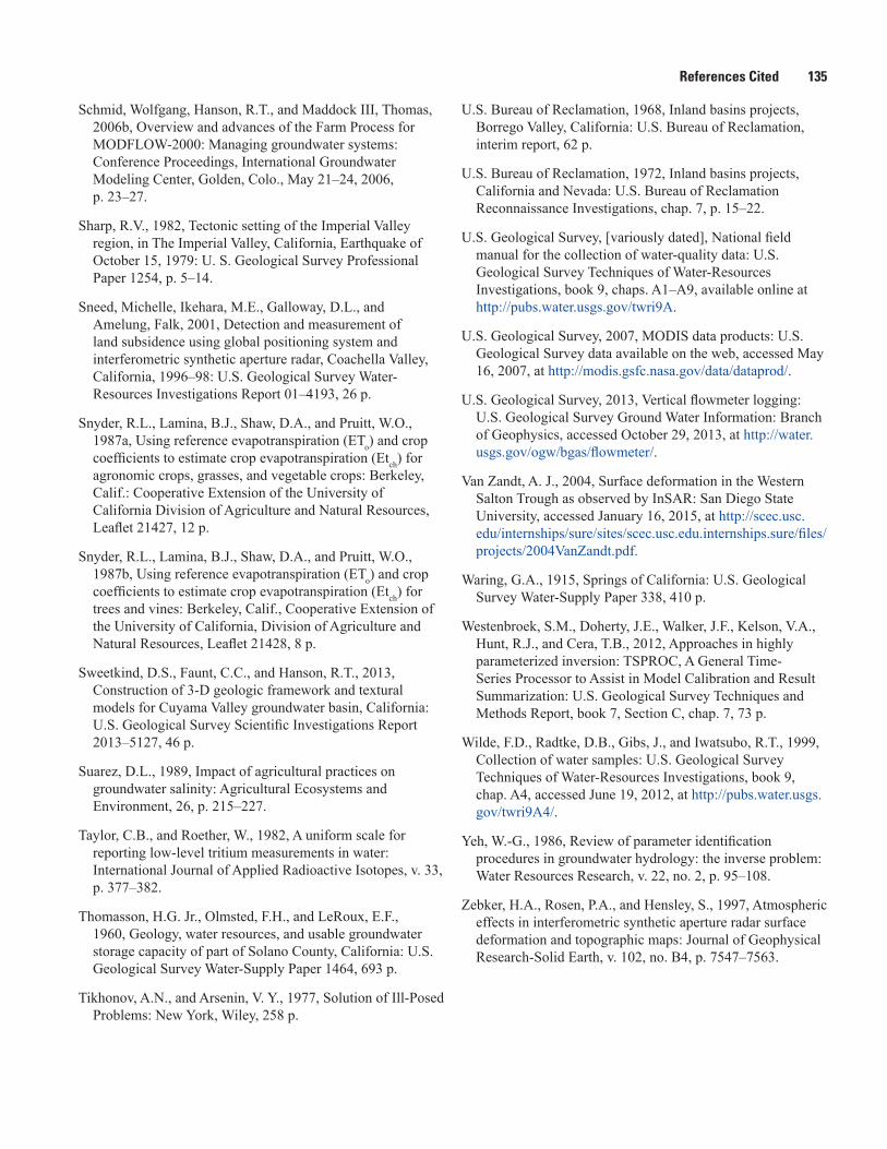
References Cited 135
Schmid, Wolfgang, Hanson, R.T., and Maddock III, Thomas, 2006b, Overview and advances of the Farm Process for MODFLOW-2000: Managing groundwater systems: Conference Proceedings, International Groundwater Modeling Center, Golden, Colo., May 21–24, 2006, p. 23–27.
Sharp, R.V., 1982, Tectonic setting of the Imperial Valley region, in The Imperial Valley, California, Earthquake of October 15, 1979: U. S. Geological Survey Professional Paper 1254, p. 5–14.
Sneed, Michelle, Ikehara, M.E., Galloway, D.L., and Amelung, Falk, 2001, Detection and measurement of land subsidence using global positioning system and interferometric synthetic aperture radar, Coachella Valley, California, 1996–98: U.S. Geological Survey Water-Resources Investigations Report 01–4193, 26 p.
Snyder, R.L., Lamina, B.J., Shaw, D.A., and Pruitt, W.O., 1987a, Using reference evapotranspiration (ETo) and crop coefficients to estimate crop evapotranspiration (Etch) for agronomic crops, grasses, and vegetable crops: Berkeley, Calif.: Cooperative Extension of the University of California Division of Agriculture and Natural Resources, Leaflet 21427, 12 p.
Snyder, R.L., Lamina, B.J., Shaw, D.A., and Pruitt, W.O., 1987b, Using reference evapotranspiration (ETo) and crop coefficients to estimate crop evapotranspiration (Etch) for trees and vines: Berkeley, Calif., Cooperative Extension of the University of California, Division of Agriculture and Natural Resources, Leaflet 21428, 8 p.
Sweetkind, D.S., Faunt, C.C., and Hanson, R.T., 2013, Construction of 3-D geologic framework and textural models for Cuyama Valley groundwater basin, California: U.S. Geological Survey Scientific Investigations Report 2013–5127, 46 p.
Suarez, D.L., 1989, Impact of agricultural practices on groundwater salinity: Agricultural Ecosystems and Environment, 26, p. 215–227.
Taylor, C.B., and Roether, W., 1982, A uniform scale for reporting low-level tritium measurements in water: International Journal of Applied Radioactive Isotopes, v. 33, p. 377–382.
Thomasson, H.G. Jr., Olmsted, F.H., and LeRoux, E.F., 1960, Geology, water resources, and usable groundwater storage capacity of part of Solano County, California: U.S. Geological Survey Water-Supply Paper 1464, 693 p.
Tikhonov, A.N., and Arsenin, V. Y., 1977, Solution of Ill-Posed Problems: New York, Wiley, 258 p.
U.S. Bureau of Reclamation, 1968, Inland basins projects, Borrego Valley, California: U.S. Bureau of Reclamation, interim report, 62 p.
U.S. Bureau of Reclamation, 1972, Inland basins projects, California and Nevada: U.S. Bureau of Reclamation Reconnaissance Investigations, chap. 7, p. 15–22.
U.S. Geological Survey, [variously dated], National field manual for the collection of water-quality data: U.S. Geological Survey Techniques of Water-Resources Investigations, book 9, chaps. A1–A9, available online at http://pubs.water.usgs.gov/twri9A.
U.S. Geological Survey, 2007, MODIS data products: U.S. Geological Survey data available on the web, accessed May 16, 2007, at http://modis.gsfc.nasa.gov/data/dataprod/.
U.S. Geological Survey, 2013, Vertical flowmeter logging: U.S. Geological Survey Ground Water Information: Branch of Geophysics, accessed October 29, 2013, at http://water.usgs.gov/ogw/bgas/flowmeter/.
Van Zandt, A. J., 2004, Surface deformation in the Western Salton Trough as observed by InSAR: San Diego State University, accessed January 16, 2015, at http://scec.usc.edu/internships/sure/sites/scec.usc.edu.internships.sure/files/projects/2004VanZandt.pdf.
Waring, G.A., 1915, Springs of California: U.S. Geological Survey Water-Supply Paper 338, 410 p.
Westenbroek, S.M., Doherty, J.E., Walker, J.F., Kelson, V.A., Hunt, R.J., and Cera, T.B., 2012, Approaches in highly parameterized inversion: TSPROC, A General Time-Series Processor to Assist in Model Calibration and Result Summarization: U.S. Geological Survey Techniques and Methods Report, book 7, Section C, chap. 7, 73 p.
Wilde, F.D., Radtke, D.B., Gibs, J., and Iwatsubo, R.T., 1999, Collection of water samples: U.S. Geological Survey Techniques of Water-Resources Investigations, book 9, chap. A4, accessed June 19, 2012, at http://pubs.water.usgs.gov/twri9A4/.
Yeh, W.-G., 1986, Review of parameter identification procedures in groundwater hydrology: the inverse problem: Water Resources Research, v. 22, no. 2, p. 95–108.
Zebker, H.A., Rosen, P.A., and Hensley, S., 1997, Atmospheric effects in interferometric synthetic aperture radar surface deformation and topographic maps: Journal of Geophysical Research-Solid Earth, v. 102, no. B4, p. 7547–7563.

This page intentionally left blank.

Prepared by the Sacramento Publishing Service Center.
For more information concerning this report, contact:
DirectorU.S. Geological SurveyCalifornia Water Science Center6000 J Street, Placer HallSacramento, CA [email protected]
or visit our Web site at:http://ca.water.usgs.gov

sac13-0509_fig40_updated
19452010
1966: Grape irrgation ends
1978: Citrus expands
Cumulative storage change
–500
Sealevel
1,000FEET
NorthwestSoutheast
Cumulative storage change
Faunt and others—H
ydrogeology, hydrologic effects of development, and sim
ulation of groundwater flow
in the Borrego Valley, San D
iego, California—Scientific Investigations Report 2015–5150ISSN 2328-0328 (online)
http://dx.doi.org/10.3133/sir20155150