Embed Size (px)
Citation preview

l
Techniques of Water-Resources Investigations
of the United States Geological Survey
Chapter C2
COMPUTER MODEL OF TWO-DIMENSIONAL SOLUTE TRANSPORT AND DISPERSION
IN GROUND WATER
By L. F. Konikow and J. D. Bredehoeft
Book 7
AUTOMATED DATA PROCESSING AND COMPUTATIONS

DEPARTMENT OF THE INTERIOR
WILLIAM P. CLARK, Secretary
U.S. GEOLOGICAL SURVEY
Dallas L. Peck, Director
Requests, at cost, for the Card Deck listed in Attachment VII should be directed to: Ralph N. Either, Chief, Office of Teleprocessing, M.S. 805, National Center,
U.S. Geological Survey, Reston, Virginia 22092.
First printing 1978 Second printing 1984
UNITED STATES GOVERNMENT PRINTING OFFICE, WASHINGTON : 1979
For sale by the Distribution Branch, U.S. Geological Survey 604 South Pick&t Street, Alexandria, VA 22304

PREFACE
The series of manuals on techniques describes procedures for plan- ning and executing specialized work in water-resources investigations. The material is grouped under major headings called books and further subdivided into sections and chapters ; section C of Book 7 is on computer programs.
This chapter presents a digital computer model for calculating changes in the concentration of a dissolved chemical species in flowing ground water. The computer program represents a basic and general model that may have to be modified by the user for efficient application to his specific field problem. Although this model will produce reliable cal- culations for a wide variety of field problems, the user is cautioned that in some cases the accuracy and efficiency of the model can be affected sig- nificantly by his selection of values for certain user-specified options.
III

CONTENTS
Abstract __________-_____-________________ Introduction _-___-_-_____-_____-__________ Theoretical background ____ ______ ---___---
Flow equation _-___I______-_______ Transport equation _______________ Dispersion coefficient, ______ -___-__ Review of assumptions ____ -_ _- ____
Numerical methods _- _____ -__-_---__-_-___ Flow equation ______ ---.._----_-_---___ Transport equation _-_-__----_-_-_-___
Method of characteristics ---__--_-_ Particle tracking _-._ ____ --_- _____ - Finite-difference approximations --_ Stability criteria ___ .____ ---- ______ Boundary and initial conditions _-__ Mass balance __-_- __.__ --_-___--___ Special problems ___._______ - _____ -
Computer program - __-__________ --_- ______ General program features ___--_-_- ____ Program segments _---__----- ____ ---__
MAIN __--___--__- _.___ ---_-_---__ Subroutine PARLOD _--- ____ - ____ Subroutine ITERAT --___-__- ____ Subroutine GENPT ____ -_- _____ -_ Subroutine VELO _ ___- _____ --___ Subroutine MOVE _______ -_-__--_-
Page 1 1 2 2 3 3 4 4 4 5 5 6 7
11 13 14 15 19 20 21 21 22 22 22 23 23
Computer program-Continued Program segments-Continued
Subroutine CNCON --_-_-__--_--__ Subroutine OUTPT ____ - __________ Subroutine CHMOT _-_----___--__
Evaluation of model ____ - ______ ---- ____ -__ Comparison with analytical solutions --_ Mass balance tests _- _______ --- _____ --
Test problem l-spreading of a tracer slug _____-______-__-_-_--------
Test problem Leffects of wells ____ Test problem 3-effects of user
options -_-______________-______ Possible program modifications -__--_-_
Coordinate system and boundary conditions --___-_-_-_---___- ____
Basic equations _- _______ -- _______ Input and output _- _____ -- ________
Conclusions ____-___________---___________ References cited _-_____--___---___________ Attachment I, Fortran IV program listing -_ Attachment II, Definition of selected program
variables _____________-_________________ Attachment III, Data input formats _-_____ Attachment IV, Input data for test problem 3 Attachment V, Selected output for test
problem 3 _______________-___-__________
FIGURES
1. Part of hypothetical finite-difference grid showing relation of flow field to movement of points--- 2. Part of hypothetical finite-difference grid showing areas over which bilinear interpolation is used
to compute the velocity at a point __________--_--______________ - __-__-___--____________ 3. Representative change in breakthrough curve from time level k-l to k ________-____________ 4. Possible movement of particles near an impermeable (no-flow) boundary ____________ --- _______ 5. Replacement of points in source cells adjacent to a no-flow boundary __-___ - __________________ 6. Replacement of points in source cells not adjacent to a no-flow boundary for negligible regional
flow (a) and for relatively strong regional flow (b) __________ -- ___________-___ -_- ______ 7. Relation between possible initial locations of points and indices of adjacent nodes _______---___ 8. Simplified flow chart illustrating the major steps in the calculation procedure ________-__-____- 9. Parts of finite-difference grids showing the initial geometry of particle distribution for the specifi-
cation of four (a), five (b), eight (c), and nine (d) particles per cell ____ - ______ -_-___-__ 10. Generalized flow chart of subroutine MOVE ---__________-____--____________________------- 11. Comparison between analytical and numerical solutions. for dispersion in one-dimensional,
steady-state flow ____________ -------------__--_----------------------------------------
Page
25 25 25 25 25 28
28 31
32 34
35 36 36 37 37 41
74 76 79
80
Page
7
7 11 15 16
17 19 21
23 24
26
V

VI CONTENTS
FIGURES-Continued 12. Comparison between analytical and numerical solutions for dispersion in plane radial steady-
13. 14. 16. 16. 17. 18. 19.
state flow ____________________-------------------------------------------------------- Grid, boundary conditions, and flow field for test problem 1 ___-- _______________-____________ Mass-balance errors for test problem 1 ___________ _-- ____ -- ____ --_-_-___--- ____ -- ___--____--_-- Grid, boundary conditions, and flow field for test problem 2 _______ -_-___-- __________--___-__-_ Mass-balance errors for test problem 2 ________ - ____________ ______________ - _-__- _ ___- _______ Grid, boundary conditions, and flow field for test problem 3 ________________ - _____ - ________- Effect of NPTPND on mass-balance error for test problem 3; CELDIk0.50 in all cases ______- Effect of CELDIS on mass-balance error for test problem 3; NPTPNDz9 in all cases -_____-__
TABLES
1. 2. 3. 4. 6.
List of subroutines for solute-transport model ________________________________________------ Model parameters for test problem 1 ________________________________________-------- - ____ Model parameters for test problems 2 and 3 ___--------__-__-__-____________________------- Effect of NPTPND on accuracy, precision, and efficiency of solution to test problem 3 ________ Effect of CELDIS on accuracy, precision, and efficiency of solution to test problem 3 ___________ 33
PEGli-3 0
28 29 30 30 31 32 33 34
Page 20 29 31 33

COMPUTER MODEL OF TWO-DIMENSIONAL SOLUTE TRANSPORT AND DISPERSION IN GROUND WATER
By L. F. Konikow and J. D. Bredehoeft
Abstract
This report presents a model that simulates solute transport in flowing ground water. The model is both general and flexible in that it can be applied to a wide range of problem types. It is applicable to one- or two-dimensional problems involving steady-state or transient flow. The model computes changes in concentration over time caused by the processes of convective transport, hydrodynamic dispersion, and mixing (or dilution) from fluid sources. The model assumes that the solute is non- reactive and that gradients of fluid density, viscos- ity, and temperature do not affect the velocity dis- tribution. However, the aquifer may be hetero- geneous and (or) anisotropic.
The model couples the ground-water flow equa- tion with the solute-transport equation. The digital computer program uses an alternating-direction im- plicit procedure to solve a finite-difference approxi- mation to the ground-water flow equation, and it uses the method of characteristics to solve the solute-transport equation. The latter uses a particle- tracking procedure to represent convective transport and a two-step explicit procedure to solve a finite- difference equation that describes the effects of hy- drodynamic dispersion, fluid sources and sinks, and divergence of velocity. This explicit procedure has several stability criteria, but the consequent time- step limitations are automatically determined by the program.
The report includes a listing of the computer pro- gram, which is written in FORTRAN IV and con- tains about 2,000 lines. The model is based on a rectangular, block-centered, finitedifference grid. It allows the specification of any number of injection or withdrawal wells and of spatially varying diffuse recharge or discharge, saturated thickness, trans- missivity, boundary conditions, and initial heads and concentrations. The program also permits the desig- nation of up to five nodes as observation points, for which a summary table of head and concentration versus time is printed at the end of the calculations. The data input formats for the model require three data cards and from seven to nine data sets to de-
scribe the aquifer properties, boundaries, and stresses.
The accuracy of the model was evaluated for two idealized problems for which analytical solutions could be obtained. In the case of one-dimensional flow the agreement was nearly exact, but in the case of plane radial flow a small amount of nu- merical dispersion occurred. An analysis of several test problems indicates that the error in the mass balance will be generally less than 10 percent. The test problems demonstrated that the accuracy and precision of the numerical solution is sensitive to the initial number of particles placed in each cell and to the size of the time increment, as determined by the stability criteria. Mass balance errors are commonly the greatest during the first several time increments, but tend to decrease and stabilize with time.
Introduction This report describes and documents a
computer model for calculating transient changes in the concentration of a nonreac- tive solute in flowing ground water. The computer program solves two simultaneous partial differential equations. One equation is the ground-water flow equation, which de- scribes the head distribution in the aquifer. The second is the solute-transport equation, which describes the chemical concentration in the system. By coupling the flow equation with the solute-transport equation, the model can be applied to both steady-state and tran- sient flow problems.
The purpose of the simulation model is to compute the concentration of a dissolved chemical species in an aquifer at any speci- fied place and time. Changes in chemical concentration occur within a dynamic ground-water system primarily due to four
1

2 TECHNIQUES OF WATER-RESOURCES INVESTIGATIONS
distinct processes : (1) convective transport, in which dissolved chemicals are moving with the flowing ground water; (2) hydro- dynamic dispersion, in which molecular and ionic diffusion and small-scale variations in the velocity of flow through the porous media cause the paths of dissolved molecules and ions to diverge or spread from the average direction of ground-water flow; (3) fluid sources, where water of one composition is introduced into water of a different composi- tion ; and (4) reactions, in which some amount of a particular dissolved chemical species may be added to or removed from the ground water due to chemical and physical reactions in the water or between the water and the solid aquifer materials. The model presented in this report assumes (1) that no reactions occur that affect the concentration of the species of interest, and (2) that gra- dients of fluid density, viscosity, and tem- perature do not affect the velocity distribu- tion.
This model can be applied to a wide variety of field problems. However, the user should first become aware of the assumptions and limitations inherent in the model, as described in this report. The computer pro- gram presented in this report is offered as a basic working tool that may have to be modified by the user for efficient application to specific field problems. The program is written in FORTRAN IV and is compatible with most high-speed computers. The data requirements, input format specifications, program options, and output formats are all structured in a general manner that should be readily adaptable to many field problems.
This report includes a detailed description of the numerical method used to solve the solute-transport equation. The reader is as- sumed to have (or can obtain elsewhere) a moderate familiarity with finite-difference methods and ground-water flow models.
Theoretical Background Flow equation
By following the derivation of Pinder and Bredehoeft (1968), the equation describing
the transient two-dimensional area1 flow of a homogeneous compressible fluid through a nonhomogeneous anisotropic aquifer can be written in Cartesian tensor notation as
$& ax? =s$+ w i,j = 1,2 (1) % J
where Tij is the transmissivity ten-
sor, L?/T; h is the hydraulic head, L ; S is the storage coefficient,
(dimensionless) ; t is the time, T; W = W (x,y,t) is the volume flux per unit
area (positive sign for outflow and negative for inflow), L/T ; and
xi and xj are the Cartesian coordi- nates, L.
If we only consider fluxes of (1) direct with- drawal or recharge, such as well pumpage, well injection, or evapotranspiration, and (2) steady leakage into or out of the aquifer through a confining layer, streambed, or lakebed, then W (x,y,t) may be expressed as
W(X,Y,-a =Q(x,zl,t) -m K”(H,-h) (2)
where Q is the rate of withdrawal (posi-
tive sign) or recharge (negative sign), L/T;
K, is the vertical hydraulic conductiv- ity of the confining layer, stream- bed, or lakebed, L/T ;
m is the thickness of the confining layer, streambed, or lakebed, L ; and
H, is the hydraulic head in the source bed, stream, or lake, L.
Lohman (1972) shows that an expression for the average seepage velocity of ground water can be derived from Darcy’s law. This expression can be written in Cartesian ten- sor notation as
(3)
c
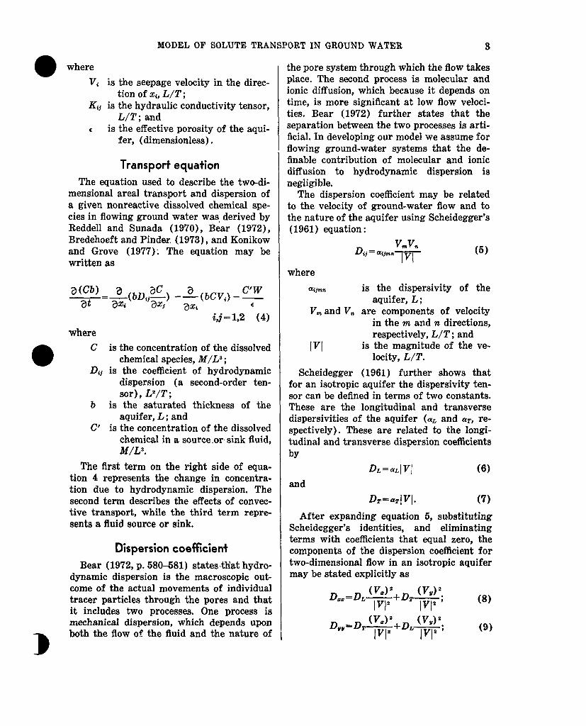
MODEL OF SOLUTE TRANSPORT IN GROUND WATER 3
where Vc is the seepage velocity in the direc-
tion of x4, L/T; K&j is the hydraulic conductivity tensor,
L/T; and c is the effective porosity of the aqui-
fer, (dimensionless).
Transport equation The equation used to describe the twsdi-
mensional area1 transport and dispersion of a given nonreactive dissolved chemical spe- cies in flowing ground water was. derived by Reddell and Sunada (1970)) Bear (1972)) Bredehoeft and Pinder (1973)) and Konikow and Grove (1977): The equation may be written as
where i,j=1,2 (4)
C is the concentration of the dissolved chemical species, M/L3 ;
Ddj is the coefficient of hydrodynamic dispersion (a second-order ten- sor), LZ/T;
b is the saturated thickness of the aquifer, L ; and
C’ is the concentration of the dissolved chemical in a sourceor, sink fluid, M/LS.
The first term on the right side of equa- tion 4 represents the change in concentra- tion due to hydrodynamic dispersion. The second term describes the effects of convec- tive transport, while the third term repre- sents a fluid source or sink.
Dispersion coefficient Bear (1972, p. 580681) states-that hydro-
dynamic dispersion is the macroscopic out- come of the actual movements of individual tracer particles through the pores and that it includes two processes. One process is mechanical dispersion, which depends upon both the flow of the fluid and the nature of
the pore system through which the flow takes place. The second process is molecular and ionic diffusion, which because it depends on time, is more significant at low flow veloci- ties. Bear (1972) further states that the separation between the two processes is arti- ficial. In developing our model we assume for flowing ground-water systems that the de- finable contribution of molecular and ionic diffusion to hydrodynamic dispersion is negligible.
The dispersion coefficient may be related to the velocity of ground-water flow and to the nature of the aquifer using Scheidegger’s (1961) equation :
TI T,
where %jmtt is the dispersivity of the
aquifer, L ; V, and V,, are components of velocity
in the m and n directions, respectively, L/T ; and
IV is the magnitude of the ve- locity, L/T.
Scheidegger (1961) further shows that for an isotropic aquifer the dispersivity ten- sor can be defined in terms of two constants. These are the longitudinal and transverse dispersivities of the aquifer (aL and aT, re- spectively). These are related to the longi- tudinal and transverse dispersion coefficients by
DL=aLlVI (6)
and DT=aTIV(. (7)
After expanding equation 5, substituting Scheidegger’s identities, and eliminating terms with coefficients that equal zero, the components of the dispersion coefficient for two-dimensional flow in an isotropic aquifer may be stated explicitly as
TIv(3 (9)

TECHNIQUES OF WATER-RESOURCES INVESTIGATIONS
vmv, D##=Dv;lr= (DL-DT)-. w
(10)
Note that while D, and D,, must have positive values, it is possible for the cross- product terms (eq 10) to have negative values if V, and V, have opposite signs.
Review of assumptions A number of assumptions have been made
in the development of the previous equa- tions. Following is a list of the main assump- tions that must be carefully evaluated before applying the model to a field problem. 1. Darcy’s law is valid and hydraulic-head
gradients are the only significant driv- ing mechanism for fluid flow.
2. The porosity and hydraulic conductivity of the aquifer are constant with time, and porosity is uniform in space.
3. Gradients of fluid density, viscosity, and temperature do not affect the velocity distribution.
4. No chemical reactions occur that affect the concentration of the solute, the fluid properties, or the aquifer proper- ties.
5. Ionic and molecular diffusion are negli- gible contributors to the total disper- sive flux.
6. Vertical variations in head and concen- tration are negligible.
7. The aquifer is homogeneous and isotropic with respect to the coefficients of longi- tudinal and transverse dispersivity.
The nature of a specific field problem may be such that not all of these underlying as- sumptions are completely valid. The degree to which field conditions deviate from these assumptions will affect the applicability and reliability of the model for that problem. If the deviation from a particular assumption is significant, the governing equations will have to be modified to account for the ap- propriate processes or factors.
Numerical Methods Because aquifers have variable properties
and complex boundary conditions, exact ana-
lytical solutions to the partial differential equations of flow (eq 1) and solute trans- port (eq 4) cannot be obtained directly. Therefore, approximate numerical methods must be employed.
The numerical methods require that the area of interest be subdivided by a grid into a number of smaller subareas. The model developed here utilizes a rectangular, uni- formly spaced, block-centered, hnite-differ- ence grid, in which nodes are defined at the centers of the rectangular cells.
Flow equation Pinder and Bredehoeft (1968) show that
if the coordinate axes are alined with the principal directions of the transmissivity tensor, equation 1 may be approximated by the following implicit finite-difference equa- tion :
where
i,j,k are indices in the x, g, and time dimensions, respec- tively ;
Ax,Ag,At are increments in the x, 2/, and time dimensions, re- spectively ; and
Go is the volumetric rate of with- drawal or recharge at the (i,j) node, L3/T.
Note that k represents the new time level and k-l represents the previous time level. To avoid confusion between tensor sub-

MODEL OF SOLUTE TRANSPORT IN GROUND WATER 6
scripts and nodal indices, the latter are sep- arated by commas.
The finite-difference equation (eq 11) is solved numerically for each node in the grid using an iterative alternating-direction im- plicit (ADI) procedure. The derivation and solution of the finite-difference equation and the use of the iterative AD1 procedure have been previously discussed in detail in the literature. Some of the more relevant refer- ences include Pinder and Bredehoeft (1968)) Prickett and Lonnquist (1971)) and Tres- cott, Pinder, and Larson (1976).
After the head distribution has been com- puted for a given time step, the velocity of ground-water flow is computed at each node using an explicit finite-difference form of equation 3. For example, the velocity in the x direction at node (i,j) would be computed as
V Km(C,j, (hi-t,i,a- j2J+1,j,d m(iA = - (12) c ZAX *
The velocity in the x direction can also be computed on the boundary between node (i,j) and node (i+l,j) using the following equation :
V K ~z(~+%J) tF, We -Jci+l,j,k )
z(i+%,i) I AX (13) c
where the hydraulic conductivity on the boundary is computed as the harmonic mean of the hydraulic conductivities at the two adjacent nodes.
Expressions similar to equations 12 and 13 are used to compute the velocities in the y direction at (i,j) and (i,j+ l/2) respectively. Note that equation 13, which computes the head difference over a distance Ax, is more accurate than equation 12, which computes the head difference over 2Ax.
Transport equation
Method of characteristics
The method of characteristics is used in this model to solve the solute-transport equa- tion. This method was developed to solve hyperbolic differential equations. If solute
transport is dominated by convective trans- port, as is common in many field problems, then equation 4 may closely approximate a hyperbolic partial differential equation and be highly compatible with the method of characteristics. Although it is difficult to present a rigorous mathematical proof for this numerical scheme, it has been success- fully applied to a variety of field problems. The development of this technique for prob- lems of flow through porous media has been presented by Garder, Peaceman, and Pozzi (1964)) Pinder and Cooper (1970)) Reddell and Sunada (1970)) and Bredehoeft and Pinder (1973). Garder, Peaceman, and Pozzi (1964) state that this technique does not introduce numerical dispersion (artifi- cial dispersion resulting from the numerical calculation process). They and Reddell and Sunada (1970) also compared solutions ob- tained using the method of characteristics with those derived by analytical methods and found good agreement for the cases in- vestigated. Applications of the method to field problems have been documented by Bredehoeft and Pinder (1973)) Konikow and Bredehoeft (1974)) Robertson (1974)) Robson (1974)) and Konikow (1977).
The approach taken by the method of char- acteristics is not to solve equation 4 directly, but rather to solve an equivalent system of ordinary differential equations. Konikow and Grove (1977, eq 61) show that by consider- ing saturated thickness as a variable and by expanding the convective transport term, equation 4 may be rewritten as
~=g-&hg)-vg
C(P -+ w- + at
c$) -~c’w
cb * (14)
Equation 14 is the form of the solute-trans- port equation that is solved in the computer program presented in this report. For con- venience we may also write equation 14 as

6 TECHNIQUES OF WATER-RESOURCES INVESTIGATIONS
where
C(Sah -+w- 2) -C’W F= at at .
cb (16)
Next consider representative fluid par- ticles that are convected with flowing ground water. Note that changes with time in prop erties of the fluid, such as concentration, may be described either for fixed points within a stationary coordinate system as successive fluid particles pass the reference points, or for reference fluid particles as they move along their respective paths past fixed points in space. Aris (1962, p. 78) states that “as- sociated with these two descriptions are two derivatives with respect to time.” Thus aC/at is the rate of change of concentration as observed from a fixed point, whereas dC/dt is the rate of change as observed when moving with the fluid particle. Aris (1962) calls the latter the material derivative.
The material derivative of concentration may be defined as
dC aC aC dx aC dy -=-++-+--* (17) dt at ax dt ay dt ’ ‘
Note the correspondence of the second and third terms on the right side of equation 15 with the second and third terms on the right side of equation 17. The latter includes the material derivatives of position, which are defined by velocity. Thus for the 2 and 2/ components, respectively, of position and velocity we have
dx -= dt
V*
and
dy v -= dt ’
(18)
(19)
If we next substitute the right sides of equations 15, 18, and 19 for the correspond- ing terms in equation 17, we obtain
-$=;&(bD$&) +F. (20)
The solutions of the system of equations comprising equations 18-20 may be given as
x=x(t) ; y=y(t) ; and C=C(t) (21)
and are called the characteristic curves of equation 15.
Given solutions to equations 18-20, a solu- tion to the partial differential equation (eq 15) may be obtained by following the char- acteristic curves. This is accomplished nu- merically by introducing a set of moving points (or reference particles) that can be traced within the stationary coordinates of the finite-difference grid. Garder, Peaceman, and‘Pozzi (1964, p. 27) state, “Each point corresponds to one characteristic curve, and values of x, y, and C are obtained as func- tions of t for each characteristic.” Each point has a concentration and position associated with it and is moved through the flow field in proportion to the flow velocity at its loca- tion. Intuitively, the method may be visual- ized as tracing a number of fluid particles through a flow field and observing changes in chemical concentration in the fluid par- ticles as they move.
Particle tracking
The first step in the method of character- istics involves placing a number of trace- able particles or points in each cell of the finite-difference grid to form a set of points that are distributed in a geometrically uni- form pattern throughout the area of inter- est. It was found that placing from four to nine points per cell provided satisfactory re- sults for most two-dimensional problems. The location or position of each particle is specified by its x- and y- coordinates in the finite-difference grid. The initial concentra- tion assigned to each point is the initial con- centration associated with the node of the cell containing the point.
For each time step every point is moved a distance proportional to the length of the time increment and the velocity at the loca- tion of the point. (See fig. 1.) The new posi- tion of a point is thus computed with the fol- lowing finite-difference forms of equations 18 and 19:
%,k= zp.k-1 + 8% = %,k--1 + AtVz[zt,,,,.vo,,,l
(22) and

MODEL OF SOLUTE TRANSPORT IN GROUND WATER 7
EXPLANATION 0 Initial location of p&tick
0 New location of particle + Flow line and direction of flow ---Computed path of particle
Figure 1 .-Part of hypothetical finite- difference grid showing relation of flow field to movement of points.
%‘,k=?h>k--l+% =7dp,k-lfAtVYrZ~p,l).v~p,*)l (23)
where P is the index number for
point identification ; and 8x, and 6~~ are the distances moved in
the x and 2/ directions, re- spectively.
The x and 2/ velocities at the position of any particular point p, indicated as ‘v~[%k,.% ?$,I9 for time k are calculated through bilinear interpolation over the area of half of a cell using the x and 2/ velocities com- puted at adjacent nodes and cell boundaries. For example, figure 2 illustrates that the velocity in the x direction of point p, located in the southeast quadrant of cell (i,i) , would be computed using bilinear interpolation be- tween the x velocities computed with equa- tions 12 and 13 at (i,i), (i,i+l), (i+1/,j), and (i+ r/&j+ 1). Similarly, the velocity in the II direction of point p would be based on the 2/ velocities computed at (i,i), (i+l,j), (i,i+$) and (i+l,j+1/2).
After all points have been moved, the con- centration at each node is temporarily as- signed the average of the concentrations of
x-
'i-l,j-1 / l l i,j-1 j l i+l,j-1 1
Y
I
. I . 1 . 1 .
EXPLANATION . Node of finite-difference grid 0 Location of particle p
-----C Xor Y Component of velocity
Area of influence for interpolating velocity in X direction at particle p
Area of influence for interpolating velocity in Y direction at particle p
Figure P.-Part of hypothetical finite-difference grid showing areas over which bilinear interpolation is used to compute the velocity at a point. Note that each area of influence is equal to one-half of the area of a cell.
all points then located within the area of that cell ; \this average concentration is denoted as Ci,j,k** The time index is distinguished with an asterisk here because this tempo- rarily assigned average concentration rep- resents the new time level only with respect to convective transport. The moving points simulate convective transport because the concentration at each node of the grid will change with each time step as different points having different concentrations enter and leave the area of that cell.
Finite-difference approximations
The total change in concentration in an aquifer may be computed by solving equa- tions M-20. Equations 18 and 19, which are related to changes in concentration caused
8 TECHNIQUES OF WATER-RESOURCES INVESTIGATIONS
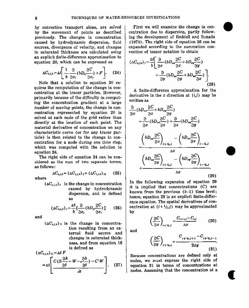
by convective transport alone, are solved by the movement of points as described previously. The changes in concentration caused by hydrodynamic dispersion, fluid sources, divergence of velocity, and changes in saturated thickness are calculated using an explicit finite-difference approximation to equation 20, which can be expressed as
AC,,j,,k = At ‘“(bD& +F ac -I . (24) Lb 3% -axj J
Note that a solution to equation 20 re- quires the computation of the change in con- centration at the tracer particles. However, primarily because of the difficulty in comput- ing the concentration gradient at a large number of moving points, the change in con- centration represented by equation 20 is solved at each node of the grid rather than directly at the location of each pomt. The material derivative of concentration on any characteristic curve (or for any tracer par- ticle) is then related to the change in con- centration for a node during one time step, which was computed with the solution to equation 24.
The right side of equation 24 can be con- sidered as the sum of two separate terms, as follows :
AC,,,,, = (AC&,,,) I+ (AC4,j,e) II (25) where
(aC,,,,,) I is the change in concentration caused by hydrodynamic dispersion, and is defined as
(26)
and (ACa,j,e) II is the change in concentra-
tion resulting from an ex- ternal fluid source and changes in saturated thick- ness, and from equation 16 is defined as
(A’%,,d,,=At 8’
=At C(S$+W-p, -C’W
at
L cb 1 * (27)
First we will examine the change in con- centration due to dispersion, partly follow- ing the development of Reddell and Sunada 1(19’70). The right side of equation 26 can he expanded according to the summation con- vention of tensor notation to obtain
Gm A finite-difference approximation for the
derivative in the x direction at (i,j) may be written as
AX (29)
In the following expansion of equation 29 it is implied that concentrations (C) are known from the previous (k-l) time level ; hence, equation 29 is an explicit finite-differ- ence equation. The spatial derivatives of con- centration at (i+ l/&j) may be approximated by
(36)
and
8 ( >
c i+w+1 -‘i+lA,j-I
ZF i+W.j= 2A1/ ’ (31)
Because concentrations are defined only at nodes, we must express the right side of equation 31 in terms of concentrations at nodes. Assuming that the concentration at a

MODEL OF SOLUTE TRANSPORT IN GROUND WATER 9
cell boundary is approximately equal to the average (arithmetic mean) of the concentra- tions at adjacent nodes, we have
C C ij+l +‘i+l,j+l
i+w+1 = (32) 2
and
C 63-l *‘i+l.j-1
c = i+%,j-1 . 2 (33)
Substitution of equations 32 and 33 into After substituting equations 30, 34, 35, and equation 31 results in : 36 into equation 29, we have
~,j+l+Ci+l.j+l -Ci,j--l-Ci+l.j--l .
4&V (34)
Similarly, the spatial derivatives of con- centration at (i - l/zJ) are
and
c&j-G-1 (35)
Ax
‘i-l,j+l +‘i.j+l -ci-l,j-l -ciej-l
4W .
(36)
bD ~=ri+W.jl(Ci+l.j-Cij) bDzzIi-%,il “i,i -ci-l.i) =
(Ax)’ - (AxI
bDzy[i+$$.j] (ci,j+l+ci+l,j+l-c~~ M-1 -ci+I,j-l)
I 4AxAy
bD *u[j-$$,j](Ci-l,j+l +’ i,j+l-Ci-l,j--l -’ G-1)
. (37) 4AxAy
A finite-difference approximation for the I
may be developed for node (i,i) in an analo- derivative in the g direction in equation 28 gous manner to equation 37 to produce
$(bDuu$+ bQ,m$$
( bDug)i,j+g -( bDu$)j,j-n ( bDuE)j,j+$4 - ( bDux$)i,j--K
= +
A2/ AlI
bD,rij+~l (C~j+l -C~j> bD,rij_ul (C,j-C.. . W-1 )
=
(AY)' - (AY)2
bD~[i,j+~](ci+lj+ci+l~+l-ci-IJ -ci-l,i+l) ,
4AxAy
bDuz[j,j,x] (‘i+*,j-1 +‘i+l j-Ct-l,j-*-Ci-l,j) , . (38)
4AxAy
Equation 28 may then be solved explicitly I
by equations 3’7 and 38 for the terms within by substituting the relationships expressed brackets on the right side of equation 28.

10 TECHNIQUES OF WATER-RESOURCES INVESTIGATIONS
Next we will examine the change in con- centration denoted by equation 27. Substi- tuting explicit finite-difference approxima- tions for the terms in equation 27, we have
(ACM) II = $[ G,,,*.+ (s[ ~J~k---$J+l ]
+ wS,,,k - l
b ha-1 bbnG -
At I) -qj,w, ik . *. ,. I (39)
Equations 28, 37, 38, and 39 together pro- vide a solution to equation 24, which in turn allows us to solve equation 20 and complete the definition of the characteristic curves of equation 15.
Because the processes of convective trans- port, hydrodynamic dispersion, and mixing are occurring continuously and simultane- ously, equations 18, 19, and 20 should be solved simultaneously. However, equations 18 and 19 are solved by particle movement based on implicitly computed heads while equation 20 is solved explicitly with respect to concentrations. Because the change in con- centration at a source node due to mixing is proportional to the difference in concentra- tion between the node and the source fluid (see eq 27)) the accuracy of estimating the concentration at the node during a time in- crement will clearly affect the computed change. Similarly, because the change in con- centration due to dispersion is proportional to the concentration gradient at a point, the accuracy of estimating the concentration
gradient will clearly affect the accuracy of the numerical results. As the position of a front or breakthrough curve advances with time, say from the k-l to k time level, the concentration gradient at any fixed reference point and the concentration differences at sources are continuosly changing. The con- sequent limitations imposed by estimating nodal concentrations in a strict explicit man- ner can be minimized by using a two-step explicit procedure in which equation 24 is solved at each node by giving equal weight to concentration gradients computed from the concentrations at the previous time level (k-l) and to concentration gradients com- puted from concentrations at time level (k*) , which represents the convected position of the front at the new time level (k) prior to adjustments of concentration for dispersion and mixing. Figure 3 illustrates the sequence of calculations to solve equations 18-20 over a given time increment. First the concentra- tion gradients at the previous time level (k- 1) are determined at each node. Then the front is convected to a new position for time level k* based on the velocity of flow and length of the time increment. Next the concentration gradients at each node are re- computed for the new position of the front. The concentrati& distribution for the new frontal position is then adjusted at each node in two steps: first based on concentration gradients at k-l and second based on con- centration gradients at k*.
The finite-difference approximation to equation 24 may thus be expressed as
1
&,,,k =
ah c(k-I) (s-+ w- $) -C’W + at
ah c,k.,(s--+ w- + at
2) -C’W
c
in which the appropriate finite-difference ap- proximations for the terms within brackets are indicated by equations 37, 38, and 39.
(40)
The new nodal concentrations at the end of time increment k are computed as
Cd,i,~= Ci,j,k* + ACi,j,k (41)
c

MODEL OF SOLUTE TRANSPORT IN GROUND WATER 11
i-
D
RELATIVE DISTANCE
Figure J.-Representative change in breakthrough curve from time level k-l to k. Note that concentration changes are exaggerated to help illustrate the sequence of calculations.
where C I,f,k. is the average of the concentra- tions of all points in cell (i,j) after equations 22 and 23 were solved for all points for time step k, and ACs,j,, is the change in concentra- tion caused by hydrodynamic dispersion, sources, and sinks, as calculated in equation 40.
Because the concentrations of points in a cell vary about the concentration of the node, the change in concentration computed at a node using equation 40 cannot be applied directly in all cases to the concentrations of the points. If the change in concentration at the node (AC& is positive, the increase is simply added to the point concentrations. But if the concentration change is negative, it is applied to points in that cell as a per- centage decrease in concentration at each point that is equal to the percentage decrease
at the node. This technique preserves a mass balance within each cell, but when a decrease in concentration is computed for a node, it will also prevent a possible but erroneous computation of negative concentrations at those points that had a concentration less than that at the node.
Stability criteria The explicit numerical solution of the
solute-transport equation has a number of stability criteria associated with it. These may require that the time step used to solve the flow equation be subdivided into a num- ber of smaller time increments to accurately solve the solute-transport equation.
First, Reddell and Sunada (1970, p. 62) show that for an explicit finite-difference solution of equation 26 to be stable,

12 TECHNIQUES OF WATER-RESOURCES INVESTIGATIONS
D,a At + D, AtL 1 ---.
(AxI (AYj2 2 (42)
Solving equation 42 for At, we see that
Substituting equation 47 into equation 45 results in 0
AS * (43)
Because the solution to equation 26 is ac- tually written as a set of iV equations for N nodes, the maximum permissible time incre- ment is the smallest At computed for any in- dividual node in the entire grid. The smallest At will then occur at the node having the largest value of
Next consider the effects of mixing ground water of one concentration with injected or recharged water of a different concentra- tion, as represented by the source terms in equation 39. The change in concentration in a source node cannot exceed the difference between the source concentration (C: j ) and the concentration in the aquifer (C,;) , and the maximum possible change occurs when a source completely flushes out the volume of water in an aquifer cell at the start of a time step. Therefore
AcijbdCijk--l -cij,. (44) . l . .
After rearranging teims in equation 44, we have
A&k 41.0. CC*,,,-1 - c’W,k)
(45)
We may isolate the effects of mixing rep- resented in equation 39 by assuming steady- state flow in which ah&t=0 and ah/at =O. Then we can rewrite equation 39 as
At wij,k (&,k--1- C’&,,k)
(&,j,d II = . b
(46) l iJ,k
After rearranging terms in equation 46, we have
(ACw.) II At W&j,k
tc :. ij,k-I-C;jk) = ‘Qk * (47)
At W4,j.k L1.O. (48)
Solving equation 48 for At at all nodes yields the following criterion :
Ai% Min b f di,k (over grid) c [ 1 ’ (49)
A third type of stability check involves the movement of points computed by equations 22 and 23 to simulate convective transport. The distance a particle moves is defined as
and 6x = At VZ[~~~,~~.Y~,,~,I (56)
6Y = At vtlrqp,gcp,~,~ . (51) In effect, this constitutes a linear spatial extrapolation of the position of a particle from one time step to the next. Where streamlines are curvilinear, the extrapolated position of a particle will deviate from the streamline on which it was previously lo- cated. .This deviation introduces an error into the numerical solution that is propor- tional to At. Thus, it is thought that an ac- curate computation of concentration changes caused by convective transport requires the maintenance of a relatively uniformly spaced field of marker particles that are moving along relatively smooth and continuous path- lines. Also, if ax is greater than Ax, or 6~ is greater than Ay, it might be possible for par- ticles to move beyond the boundaries of the grid during one time increment. Thus, for a given velocity field and grid, some restric- tion must be placed on the size of the time increment to assure that neither 8x nor Sy exceed some critical distances, called Sx*and Sz/*. Therefore
sx4x* (52) and
ayay*. (53) These critical distances can be related to
the dimensions of the finite-difference grid by
8x* = yAx (54) and

MODEL OF SOLUTE TRANSPORT IN GROUND WATER 13
&*=yAy (55) where y is the fraction of the grid dimen- sions that particles will be allowed to move (0 < y& 1).
If we replace the terms in equations 52 and 53 with the corresponding terms from equations 50, 51,54, and 55, we have
and At vz[z cp,r,%.,sJ LYAX (56)
At VYr2,p.*,.r(,,*,l --LYAY- (57) Because these criteria are governed by the maximum velocities in the system, and since the computed velocity of a tracer particle will always be less than or equal to the maximum velocity computed at a node or celh boundary, we have to check only the latter. Substituting the grid velocities and solving equations 56 and 57 for At results in
and
Ai% $; (53) a max
(59)
If the time step used to solve the flow equation exceeds the smallest of the time limits determined by equations 43, 49, 58, or 59, then the time step will be subdivided into the appropriate number of smaller time in- crements required for solving the solute- transport equation.
Boundary and initial conditions
Obtaining a solution to the equations that describe ground-water ilow and solute trans- port requires the specification of boundary and initial conditions for the domain of the problem. Specifications for solving the flow equation must be compatible with the solu- tion of the solute-transport equation. Several different types of boundary conditions can be incorporated into the solute-transport model. Two general types are incorporated in this model ; these are constant-flux and constant-head conditions. These can be used to represent the real boundaries of an aquifer as well as to represent artificial
3 boundaries for the model.- The use of the
latter can help to minimize data require- ments and the area1 extent of the modeled part of the aquifer.
A constant-flux boundary can be used to represent aquifer underflow, well with- drawals, or well injection. A finite flux is designated by specifying the flux rate as a well discharge or injection rate for the appro- priate nodes. A no-flow boundary is a spe- cial case of a constant-flux boundary. The numerical procedure used in this model re- quires that the area of interest be sur- rounded by a no-flow boundary. Thus the model will automatically specify the outer rows and columns of the finite-difference grid as no-flow boundaries. No-flow boundaries can also be located elsewhere in the grid to simulate natural limits or barriers to ground-water flow. No-flow boundaries are designated by setting the transmissivity equal to zero at appropriate nodes, thereby precluding the flow of water or dissolved chemicals across the boundaries of the cell containing that node.
A constant-head boundary in the model can represent parts of the aquifer where the head will not change with time, such as re- charge boundaries or areas beyond the in- fluence of hydraulic stresses. In this model constant-head boundaries are simulated by adjusting the leakage term (the last term on the right side of equation 11) at the appro- priate nodes. This is accomplished by setting the leakance coefficient (Z&/m) to a suffi- ciently high value (such as 1.0 s-l) to allow the head in the aquifer at a node to be im- plicitly computed as a value that is essen- tially equal to the value of H,, which in this case would be specified as the desired con- stant-head altitude. The resulting rate of leakage into or out of the designated con- stant-head cell would equal the flux required to maintain the head in the aquifer at the specified constant-head altitude.
If a constant+flux or constant-head bound- ary represents a fluid source, then the chemi- cal concentration in the source fluid (C’) must also be specified. If the boundary rep- resents a fluid sink, then the concentration of the produced fluid will equal the concen-

14 TECHNIQUES OF WATER-RESOURCES INVESTIGATIONS
tration in the aquifer at the location of the sink.
Because solute transport directly depends upon hydraulic and concentration gradients, the head and concentration in the aquifer at the start of the simulation period must be specified. The initial conditions can be deter- mined from field data and (or) from previ- ous simulations. It is important to note that the simulation results may be sensitive to variations or errors in the initial conditions. In discussing computed heads, Trescott, Pinder, and Larson (1976, p. 30) state:
If initial conditions are specified so that transient flow is occurring in the system at the start of the simulation, it should be recognized that water levels will change during the simulation, not only in re- sponse to the new pumping stress, but also due to the initial conditions. This may or may not be the irkent of the user.
Mass balance Mass balance calculations are performed
after specified time increments to help check the numerical accuracy and precision of the solution. The principle of conservation of mass requires that the cumulative sums of mass inflows and outflows (or net flux) must equal the accumulation of mass (or change in mass stored). The difference between the net flux and the mass accumulation is the mass residual (R,) and is one measure of the numerical accuracy of the solution. Al- though a small residual does not prove that the numerical solution is accurate, a large error in the mass balance is undesirable and may indicate the presence of a significant error in the numerical solution.
The model uses two methods to estimate the error in the mass balance. Both are based on the magnitude of the mass residual, R,, which is computed from
where
R,=AM,-M, (60)
AM, is the change in mass stored in the aquifer, M; and
Mt is the net mass flux, M.
The two mass terms, AM, and MI, are evaluated using the following equations :
where C,j,, is the initial concentration at node (i,j) , M/L3 ; and
M,=888Wc,j,khXayatk cij k Cjk ,I . (6lb)
The percent error (E) in the mass bal- ance is computed first by comparing the residual with the average of the net flux and net accumulation, as
E JOO.O(M,--a,) 1
O.~(M,+AMJ ' (62)
This is a good measure of the accuracy of the numerical solution when the flux and the change in mass stored are relatively large. However, equation 62 does not account for the initial mass of solute in the aquifer. If total fluxes are very small compared to the initial mass of solute in the aquifer, then equation 62 might indicate a relatively large error when the numerical solution is actually quite accurate. Therefore, the error may also be computed a second way by comparing the residual with the initial mass of solute (Mo) present in the aquifer, as
E 2 =lOO.O (M,-AM,)
Mo * (63)
Equation 63 provides a good measure of the accuracy of the numerical solution when fluxes are zero or relatively small. But when M, is zero or very small in comparison to AM,, then E, becomes meaningless. This problem can be overcome by correcting M, in the denominator of equation 63 for the net mass flux, resulting in
E =lOO.W,-alM,) 3
M,,-M, * (64
Note that as M, becomes very small, equa- tion 64 approaches equation 63, and as M. becomes very small, E, becomes just a com- parison of the residual with the net flux. In the latter case E, is a mass balance indicator similar to E, in equation 62. Thus, E, is con- sidered a more reliable and versatile indi- cator of numerical accuracy than is Ez. Either one or both of E, and E, are computed by the model, as appropriate.

MODEL OF SOLUTE TRANSPORT IN GROUND WATER 15
Special problems
There are a number of special problems associated with the use of the method of characteristics to solve the solute-transport equation. Some of these problems are asso- ciated with the movement and tracking of particles, while other problems are related to the computational transition between the concentrations of particles within a cell and the average concentration at that node. We will next describe the more significant prob- lems and the procedures used to minimize errors that might result from them.
One possible problem is related to no-flow boundaries. Neither water nor dissolved chemicals can be allowed to cross a no-flow boundary. However, under certain conditions it might be possible for the interpolated velocity at the location of a particle near a no-flow boundary to be such that the particle will be convected across the boundary during one time increment. Figure 4 illustrates such a possible situation, which arises from the deviation between the curvilinear flow line and the linearly projected particle path. If a particle is convected across a no-flow boundary, then it is relocated within the aquifer by reflection across the boundary, as also shown in figure 4. This correction thus will tend to relocate the particle closer to the true flow line.
Fluid sources and sinks also require special treatment. Because they tend to represent, singularities in the velocity field, the use of a central difference formulation (eq 12) to compute the velocity at a node may indicate zero or very small velocities at the nodes. Therefore, the velocity components at a source or sink node cannot be used for in- terpolation of the velocity at a point within or adjacent to that cell. To help maintain radial flow to or from a sink or source, re- spectively, the velocities computed on the boundaries of source or sink cells are as- signed to that node. The appropriate bound- ary velocities are determined on the basis of the quadrant of interest. This can be illus- trated by referring again to figure 2. If a point is located in the southeast quadrant of cell (i,i), the x velocity at node (iJ) would
.
EXPLANATION . Node of finite-difference grid a Previous location of particle p
0 Computed new location of particle p A Corrected new location of particle p
b Flow line and direction of flow --- Computed path of flow
N Zero transmissivity (or no-f low boundary)
Figure 4.-Possible movement of particles near an impermeable (no-flow) boundary.
be set equal to V
V7/(ii+M) *
z(i+M j,and the 9 velocity to Corresponding adjustments are
made for points in other quadrants, so that the magnitude and direction of velocity at the node are not fixed for a given time in- crement, but depend on the relative location of the point of interest within the cell. A similar approximation is made when a point of interest is located in a cell adjacent to a source or sink. Thus, if the same point, p, in figure 2 were located in an unstressed cell but the adjacent cell (i+l,j) represented a source or sink, then the y velocity at node (i+ l,i) would be approximated by
%+1 i+ 5) in order to estimate the y velocity
at point p. A corresponding approximation for the x velocity at node (i,i+ 1) would be made using Vsci+‘A j+l)if a source or sink were located at (i,ii 1).
The maintenance of a reasonably uniform and continuous spacing of points requires special treatment in areas where sources and sinks dominate the flow field. Points will con- tinually move out of a cell that represents a source, but few or none will move in to re-

16 TECHNIQUES OF WATER-RESOURCES INVESTIGATIONS
place them and thereby maintain a continuous stream of points. Thus, whenever a point that originated in a source cell moves out of that source cell, a new point is introduced into the source cell to replace it. Placement of new points in a source cell is compatible with and analogous to the generation of fluid and solute mass at the source.
The procedure used to replace points in source cells that are adjacent to no-flow boundaries is illustrated in figure 5. Here a steady, uniformly spaced stream of points is maintained by generating a new point at the same relative position in the source cell as the new position in the adjacent cell of the point that left the source cell. As an example, point ‘7 was convected from cell (i- l,i) to cell (i,i) . So the replacement point (22) was placed at a location within cell (i-1,j) that is identical to the new location of point 7 within cell (i,j) .
The procedure used to replace points in source cells that lie within the aquifer and not adjacent to a no-flow boundary is illus- trated in figure 6. Here a steady, uniformly spaced stream of particles is maintained by generating a new point in the source cell at the original location of the point that left the source cell. When a relatively strong
time k-l
source is imposed on a relatively weak re- gional flow field, as illustrated in figure 6a, then radial flow will be maintained in the area of the source, and all initial and replace- ment points will move symmetrically away from node (i,j). For example, after point 7 moves from cell (i,i) to (i+l, i-l), the re- placement point (18) is positioned at time k in cell (i,i) at the same location as the ini- tial position of point ‘7. Although the re- placement procedure illustrated earlier by figure 5 would work just as well for the case illustrated in figure 6a, it would not be satis- factory for the situation presented in figure 6b, which illustrates the imposition of a rela- tively weak source in a relatively strong regional flow field. In this case the velocity distribution within the source cell does not possess radial symmetry, and the velocity within the upgradient part of the source cell is much lower than the velocity within the d,owngradient part of the source cell. Re- placement of points at original locations in source cells, as illustrated in figure 6b, will maintain a steady stream of points leaving the source cell in proportion to the velocity field. However, the use of the procedure illus- trated in figure 5 for the case presented in figure 6b would result in the accumulation of
time k
EXPLANATION . Node of finite-difference gid
n p initial location Of psrticle P Op New location of particle P Ap Location of replacement particle p
q Cmsmnt -head source
018 .
.
04
OS
t
l
014
019
.
Figure &-Replacement of points in source cells adjacent to a no-flow boundary. c

MODEL OF SOLUTE TRANSPORT IN GROUND WATER 17
time k-l
time k-l
time k
-01 ‘2 ‘i.j-1 ‘3
6. o7 :
OS
time I(
.j-1
EXPLANATION
. Node of finite-difference grid
8p Initial location of particle p I&, New location of particle p *P Location of replacement particle p
Fluid oourco
Figure 6.-Replacement of points in source cells not adjacent to a no-flow boundary for negligible regional flow (a) and for relatively stroyg regional flow (b).
points in the low-velocity area of the source cell (i,i) , with few points being replaced into the high-velocity area, where convective transport is the greatest.
Although we normally expect points to be convected out of source cells, figure 6b also demonstrates the possibility that points may sometimes enter a source cell. This can also occur when two or more source cells of dif- ferent strengths are adjacent to each other. An erroneous multiplication of points might then result if points that did not originate in a particular source cell are replaced when
they in turn are convected out of that source cell. Therefore, points leaving a source cell are replaced only if they had originated in that source cell.
Hydraulic sinks also require some special treatment. Points will continually move into a cell representing a strong sink, but few or none will move out. To avoid the resultant crowding and stagnation of tracer points, any point moving into a sink cell is removed from the flow field after the calculations for that time increment have been completed.
i The numerical removal of points which enter

18 TECHNIQUES OF WATER-RESOURCES INVESTIGATIONS
sink cells is analogous to the withdrawal of fluid and solute mass through the hydraulic sink. The combination of creating new points at sources and destroying old points at sinks will tend to maintain the total number of points in the flow field at a nearly constant value.
Both the flow model and the transport model assume that sources and sinks act over the entire cell area surrounding a source or sink node. Thus, in effect, heads and concentrations computed at source or sink nodes represent average values over the area of the cell. Part of the total concentra- tion change computed at a source node repre- sents mixing between the source water at one concentration and the ground water at a different concentration (eq 39). It can be shown from the relationship between the source concentration ( C,:i,k ) and the aquifer concentration (Ci,j,k-1) , as indicated by equation 44, that the following constraints generally must be met in a source cell:
c ti.k LC’
ijk * 9 for ‘:jk >Ci,j,k--l VW * .
and cijk~C’ijk for Cijk <Cijkel. (65b) * . . , , . 9 .
If it is assumed that the sources act over the area of the source cell and that there is complete vertical mixing, then these same constraints should also apply to all points within the cell. Because of the possible devia- tion of the concentrations of individual points within a source cell from the average concentration, the change in concentration cqmputed at a source node (AC,,& should not be applied directly to each of the points in the cell. Rather, at the end of each time increment the concentration of each point in a source cell is updated by setting it equal to the final nodal concentration. Although this may introduce a small amount of nu- merical dispersion by eliminating possible concentration variations within the area of a source cell, it prevents the adjustment of the concentration at any point in the source cell to a value that would violate the constraints indicated by equation 65.
In areas of divergent flow there may be a problem because some cells can become void
of points where pathlines become spaced a widely apart. This would result in a calcula- tion of zero change in concentration at a node due to convective transport, although the nodal concentration would still be ad- justed for changes caused by hydrodynamic dispersion (eq 28). Also, some numerical dispersion is generated at nodes in and ad- jacent to the cells into which the convective transport of solute was underestimated be- cause of the resulting error in the concentra- tion gradient. This might not cause a serious problem if only a few cells in a large grid ‘became void or if the voiding were transitory (that is, if upgradient points were convected into void cells during later or subsequent time increments). Figure 6a illustrates radial flow, which represents the most severe case of divergent flow. Here it can be seen that when four points per cell are used to simulate convect,ive transport, then in the numerical procedure four of the eight sur- rounding cells would erroneously not receive any solute by convection from the adjacent source. If eight points per cell were used initially, then at a distance of two rows or columns from the source only 8 of 16 cells would be on pathlines originating in the source cell. So, while increasing the initial number of points per cell would help, it is obvious that for purely radial flow, an im- practically large initial number of points per cell would be required to be certain that at least one particle pathline passes from the source through every cell in the grid.
The problem of cells becom,ing void of par- ticles can be minimized by limiting the num- ber of void cells to a small percentage of the total number of cells that represent the aquifer. If the limit is exceeded, the numeri- cal solution to the solute-transport equation is terminated at the end of that time incre- ment and the “final” concentrations at that t,ime are saved. Next the problem is reini- tialized at the time of termination by re- generating the initial particle distribution throughout the grid and assigning the “final” concentrations at the time of termination as new “initial” concentrations for nodes and particles. The solution to the solute-transport

MODEL OF SOLUTE TRANSPORT IN GROUND WATER 19
equation is then simply continued in time from this new set of “initial” conditions until the total simulation period has elapsed. This procedure preserves the mass balance within each cell but also introduces a small amount of numerical dispersion by eliminating vari- ations in concentration within individual cells.
To help minimize the amount of numer,i- cal dispersion resulting from the regenera- tion of points, the program also includes an optimization routine that attempts to main- tain an approximation of the previous con- centration gradient within a cell. The opti- mization routine aims to meet the following constraints :
SC; n=l
-=G,j NP
(6W
c, ,Ic*Lc ’ n t,m for C&G,,,, (66b) and
Cl mLCn*IC4,1 I for C$Cl,m (66c) where
C,* is the concentration of the nth point in cell (i,j) , M/L3 ;
NP is the total number of points ini- tially placed in a cell ; and
C Lm is the concentration at node (Z,m), which represents a cell adjacent to (i,j) and on a line that starts at (i,j) and extends through the coordinates of the point (n) of interest, as illustrated in figure 7, M/L3.
Note that equation 66a simply indicates that a mass balance must be preserved in a cell regardless of the range in variation of point concentrations within the cell. Equa- tions 66b and c indicate that the concentra- tion of any point must lie between Ct,, and the concentration at the node adjacent to particle n. The coordinates of the adjacent node would take on values of l=i or l=i+ 1 and m= i or m= j f 1. For example, figure 7 shows that for point 2, the coordinates (I+) would equal (i,i - 1)) while for point 3, (Z,m) would equal (i+ 1,j - 1) . The optimization
.
.
.
f i. j-1
/’ i+l,i-1
/
I /
/
! /
/ I /
.
‘6 ‘7 ‘6
. I .
EXPLANATION . Node of finite -difference grid
mn Location of particle n
Figure 7.-Relation between possible ini- tial locations of points and indices of ad- jacent nodes.
routine is written so that if equations 66a-c cannot be satisfied simultaneously for node (i,j) within two iterations, then to avoid fur- ther computational delay all C: are simply set equal to C4+
Computer Program The computer program serves as a means
of translating the numerical algorithm into machine executable instructions. The pur- pose of this chapter is to describe the overall structure of the program and to present a detailed description of its key elements, thereby providing a link between the numeri- cal methods and the computer code. We hope that this link will make it easier for the model user to understand and, if necessary, modify the program. The FORTRAN IV source program developed for this model is listed in attachment I and includes almost 2,000 lines. For reference purposes columns 73-80 of each line contain a label that is numbered sequentially within each sub- routine. The definition of selected variables used in the program is presented in attach- ment II ; this glossary therefore also serves as a key for relating the program variables

20 TECHNIQUES OF WATER-RESOURCES INVESTIGATIONS
to their corresponding mathematical terms. The computer program is compatible with many scientific computers ; it has been suc- cessfully run on Honeywell, IBM, DEC, and CDC computers.
General program features
The program is segmented into a main routine and eight subroutines. The name and primary purpose of each segment are listed in Table 1. Each program segment will be described in more detail in later sections of this chapter.
Table l.-List of subroutines for solute-transport model
NMIle Purpose
MAIN ----Control execution. PARLOD --Data input and initialization. ITERAT ---Compute head distribution. GENPT --Generate or reposition particles. VELO ---Compute hydraulic gradients, velocities,
dispersion equation coefficients, and time increment for stable solution to transport equation.
MOVE -----Move particles. CNCON ___ Compute change in chemical concentra-
tions and compute mass balance for transport model.
OUTPT ---Print head distribution and compute mass balance for flow model.
CHMOT ---Print concentrations, chemical mass balance, and observation well data.
The major steps in the calculation pro- cedures are summarized in figure 8, which presents a simplified flow chart of the over- all structure of the computer program. The flow chart illustrates that the tracer particles may have to be moved more than once to complete a given time step. In other words, the time step used to implicitly solve the flow equation may have to be subdivided into a number of smaller time increments for the explicit solution of the solute-transport equation. The maximum time increments al- lowable for the explicit calculations are com- puted automatically by the model. Thus, the model user cannot specify an erroneously large increment or an inefficiently small in-
crement for solving the solute-transport equation. For transient flow problems, some discretion is still required in the specifica- tion of the initial time step and of the time- step multiplier, as discussed by Trescott, Pinder, and Larson (1976, p. 38-40).
The general program presented here is written to allow a grid having up to 20 rows and 20 columns. Because the numerical pro- cedure requires that the outer rows and col- umns represent no-flow boundaries, the aquifer itself is then limited to maximum dimensions of 18 rows and 18 columns. If a problem requires a larger grid, then the ap- propriate arrays must be redimensioned ac- cordingly. These arrays are contained in COMMON statements PRMK, HEDA, HEDB, CHMA, CHMC, and DIFUS, and in DIMENSION statements on lines C170, G200, H140, and 1160.
The program allows the specification of one pumping well per node. The wells can represent injection (recharge) or withdrawal (discharge). If more than one well exists within the area of a cell, then the flux spe- cified for that node should represent the net rate of injection or withdrawal of all wells in that cell. The model assumes that stresses are constant with time during each pumping period (NPMP) . But the total number of wells, as well as their locations, flux rates, and source concentrations, may be changed for successive pumping periods. The pro- gram also allows the specification of obser- vation wells at as many as five nodes in the grid. For nodes that are designated as ob- servation wells, at the end of the simulation period or after every 50 time increments the model will print a summary table of the head and concentration at the previous time in- crements.
The program also includes a node identi- fication array (NODEID), which allows cer- tain nodes or zones to be identified by a unique code ,number. This feature can save much time in the preparation of input data by easily equating each code number with a desired boundary condition, flux, or source concentration.

MODEL OF SOLUTE TRANSPORT IN GROUND WATER 21
READ GEOLOGIC, HYDROLOGIC,&
I GENERATE UNIFORM COMPUTE HYDRAULIC DISTRIBUTION OF GRADIENTS FOR
TRACER PARTICLES l-4 ONE TIME STEP l- c , k
+
,
, COMPUTE DISPERSION COMPUTE
EQUATION COEFFICIENTS GROUND- WATER
A VELOCITIES
COMPUTE AVERAGE CONCENTRATION IN EACH FINITE-DIFFERENCE CELL
c COMPUTE EXPLICITLY
THE CHEMICAL CONCE(;:RDA;CSlON AT
c ADJUST CONCENTRATION
OF EACH PARTICLE
I
+ COMPUTE
MASS BALANCE 1
NO
I I +YES T
SUMMARIZE AND PRINT RESULTS
I
c
STOP
Flgure &-Simpllfied flow chart illustrating the major steps in the calculation procedure.
Program segments of the program. Subroutines for input, ex-
MAIN ecution, and output are called from MAIN and the elapsed time simulated is compared
The primary purpose of the MAIN routine with the desired total simulation period. is to control the overall execution sequence Also, lines ASOO-A580 serve to store (or

22 TECHNIQUES OF WATER-RESOURCES INVESTIGATIONS
record) observation well data for transient flow problems.
Subroutine PARLOD
All input data are read through subroutine PARLOD. These data define the properties, boundaries, initial conditions, and stresses for the aquifer, as well as spatial grid and time-step factors. The values of many vari- ables are also initialized here. After the data are read, some preliminary calculations are made, such as (1) determining time incre- ments for the flow model (lines B780-B890), (2) computing the harmonic mean trans- missivities in the 2 and 2/ directions (B1670- BMOO) , (3) adjusting transmissivity for anisotropy (B1810-B1820), (4) computing iteration parameters (B1840-B1910 and B2880-B2980), and (5) checking for possible inconsistencies among the i n p u t data (B3140-B3290). A printout is also provided of all input data so that the data may be re- checked and each run identified.
Subroutine ITERAT
This subroutine solves a finite-difference approximation of the flow equation (eq 11) using an iterative AD1 procedure. The ma- trix generated by the finite-difference ap- proximation is solved using the Thomas algorithm, as described by von Rosenberg (1964, p. 113). Row calculations are made in lines C270-C610, and column calculations are made in lines C630-C970. The calculations are assumed to have converged on a solution if the maximum difference at all nodes be- tween heads computed along rows and heads computed along columns is less than the spec- ified tolerance. Convergence is checked on lines C940-C960. Note that here (for ex- ample, lines C380, C700, C930, and C1150) and in other subroutines the thickness array (THCK) is used to check whether a node is in the aquifer.
It should also be noted here that the flow model, as written, assumes that the trans- missivity of the aquifer is independent of the head (or saturated thickness) and remains constant with time. If this assumption is not
to the particular aquifer system ‘being-modeled, then the solution algorithm presented in this subroutine should be modi- fied accordingly. For example, flow models published by Prickett and Lonnquist (1971, p. 43-45) and Trescott, Pinder, and Larson (1976) include such a modification.
All parameters involved in the calculation of heads are defined as double precision vari- ables and all calculations involving these parameters are performed in double pre- cision. The number of double precision vari- ables and operations can be reduced sig- nificantly if the program is to be executed on a high-precision scientific computer, thereby improving the efficiency of the model by re- ducing computer storage requirements and execution time.
The iterative AD1 procedure used to solve the finite-difference equations is not neces- sarily the best possible solution technique for all problems. For example, it may be difficult to obtain a solution using the iterative AD1 procedure for cases of steady-state flow when internal nodes in the grid have zero trans- missivity and for cases in which the trans- missivity is highly anisotropic. In such cases, a strongly implicit procedyre, such as the one documented by Trescott, Pinder, and Larson (1976)) should ,be substituted for the solution algorithm contained in subroutine ITERAT.
Subroutine GENPT
The primary purpose of subroutine GENPT is to generate a uniform initial distribution of tracer particles throughout the finite-difference grid. This is done either at the start of a simulation period or at an intermediate time when too many cells have become void of particles. In the latter case, the program attempts to preserve an ap proximation of the previous concentration gradient within each cell (lines D1420-
: D2040). The placement of particles is accomplished
“in lines D!XO-D1410. The program allows the placement of either four, five, eight, or nine particles per cell. Of course each option will result in a slightly different geometry
c

l . . . . . . T . . . . . .
. . .
. . .
#
. . .
. . .
A
MODEL OF SOLUTE TRANSPORT IN GROUND WATER 23 . . . . . . . . . . . . . . . . . at . . . . . . . . . . . . . . . . . . . B ...... .......... .......... ..........
.......... m ..........
...... ..........
.......... ..........
. l ........ ..........
...... ..........
C D
Figure 9.-Parts of finite-difference grids showing the initial geometry of particle distribution for the specification of four (A), five (B), eight (C), and nine (0) particles per cell.
and density of points, as illustrated by figure 9. The most regular or uniform patterns are produced when four or nine particles per cell are specified. If a different number of par- ticles per cell or a different placement geom- etry are desired, this subroutine could be modified accordingly.
As particles are moved or convected through the grid during the calculation pro- cedure, there is a need to remove particles at fluid sinks and create particles at fluid sources. A buffer array (called LIMBO) is created on lines D430-D480 that contains particles that can be added later to the grid at sources and that also contains space to store particles removed at sinks or discharge boundaries.
Subroutine VELO Subroutine VELO accomplishes three ob-
jectives. First, it computes the flow velocities at nodes and on cell boundaries by solving equations having the form of equations 12 and 13. The velocities are computed on lines E420-E680. Second, the dispersion equation coefficients are calculated. These coefficients represent terms factored out of equations 37 and 38, as follows : DISPUXJYJ) = (bD,J ri+n,j,/(Az)e (67s)
3 DISP(IX,IY,2) = W,,) cij+w,/(4/)2 t67b)
DISP(IX,IY,S) = (bD,) ri+nd,/4AXAy (67~) DISP(IX,IY,4) = (b&J tii+n,/4AXAy. (67d) Note that each dispersion coefficient (Dm, D,, D, D,) is computed on cell boundaries using the relationships expressed in equa- tions 8-10. Therefore, the equation coeffi- cients computed by equation 67 are stored as forward values from the indicated node in the DISP array. Third, this subroutine com- putes (on lines E1050-El240 and E1800- E1930) the minimum number of particle moves (NMOV) required to solve the trans- port equation for the given time step so that the maximum time increment for the trans- port equation solution will not exceed any of the criteria indicated by equations 43, 49, 58, and 69.
Subroutine MOVE
Although this subroutine has only one main function, which is to move the tracer par- ticles in accordance with equations 22 and 23, it is the longest and perhaps the most complex segment of the program. The com- plexities are mainly introduced by the treat- ment of particles at the various types of boundary conditions. To help illustrate the calculation procedure followed within sub- routine MOVE, a flow chart is presented in figure 10. The numbers in the flow chart in- dicate the corresponding lines in subroutine MOVE where the indicated operation is executed.
If a node represents a fluid source or sink, then particles must be respectively created or destroyed in these cells. If the value of pumpage (REC) at a node does not equal zero, then the node is assumed to represent either a fluid source (for REC<O) or a fluid sink (for REC>O) . Recharge or discharge can also be represented by the RECH array. But it is assumed that this type of flux is sufficiently diffuse so that it does not induce areas or points of strongly divergent or con- vergent flow and therefore particles need not be created or destroyed at these nodes. Note that here and in other subroutines the pres- ence of a constant-head boundary is tested by checking the value of leakance (VPRM)

24 TECHNIQUES OF WATER-RESOURCES INVESTIGATIONS
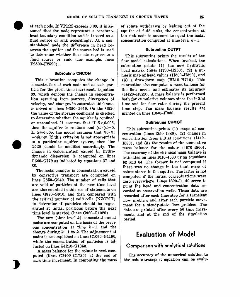
MODEL OF SOLUTE TRANSPORT IN GROUND WATER 26
at each node. If VPRM exceeds 0.09, it is as- sumed that the node represents a constant- head boundary condition and is treated as a fluid source or sink accordingly. At a con- stant-head node the difference in head be- tween the aquifer and the source bed is used to determine whether the node represents a fluid source or sink (for example, lines F2500-F2520).
Subroutine CNCON This subroutine computes the change in
concentration at each node and at each par- ticle for the given time increment. Equation 39, which denotes the change in concentra- tion resulting from sources, divergence of velocity, and changes in saturated thickness, is solved on lines G350-G610. On the G520 the value of the storage coefficient is checked to determine whether the aquifer is confined or unconfined. It assumes that if S<O.O05, then the aquifer is confined and ah/at= 0. If S10.005, the model assumes that @/at =ah/at. If this criterion is not appropriate to a particular aquifer system, then line G.520 should be modified accordingly. The change in concentration caused by hydro- dynamic dispersion is computed on lines G640-G770 as indicated by equations 37 and 38.
The nodal changes in concentration caused by convective transport are computed on lines G850-G940. The number of cells that are void of particles at the new time level are also counted in this set of statements on lines GBBO-G910, and then compared with the critical number of void cells (NZCRIT) to determine if particles should be regen- erated at initial positions before the next time level is started (lines G960-G1020).
The new (time level k) concentrations at nodes are computed on the basis of the previ- ous concentration at time k- 1 and the change during k - 1 to k. The adjustment at nodes is accomplished on lines G1060-Gl180, while the concentration of particles is ad- justed on lines G1210-G1360.
A mass balance for the solute is next corn. puted (lines G1400-G1730) at the end 01 each time increment. In computing the mash
)f solute withdrawn or leaking out of the aquifer at fluid sinks, the concentration at ;he sink node is assumed to equal the nodal :oncentration computed at time level k - 1.
Subroutine OUTPT This subroutine prints the results of the
Row model calculations. When invoked, the subroutine prints (1) the new hydraulic head matrix (lines H190-H260), (2) a nu- meric map of head values (H300-H390), and (3) a drawdown map (H510-H710). This subroutine also computes a mass balance for the flow model and estimates its accuracy (H420-H820). A mass balance is performed both for cumulative volumes since the initial time and for flow rates during the present time step. The mass balance results are printed on lines H840-H930.
Subroutine CHMOT This subroutine prints (1) maps of con-
centration (lines 1250-1380)) (2) change in concentration from initial conditions (1440- 1580), and (3) the results of the cumulative mass balance for the solute (1670-1860). The accuracy of the chemical mass balance is estimated on lines 1610-1660 using equations 62 and 64. The former is not computed if there was no change in the total mass of solute stored in the aquifer. The latter is not computed if the initial concentrations were zero everywhere. Lines 1890-11140 serve to print the head and concentration data re- corded at observation wells. These data are recorded after each time step for a transient flow problem and after each particle move- ment for a steady-state flow problem. The data are printed after every 50 time incre- ments and at the end of the simulation period.
Evaluation of Model
Comparison wiih analytical solutions
The accuracy of the numerical solution to the solute-transport equation can be evalu-

26 TECHNIQUES OF WATER-RESOURCES INVESTIGATIONS
ated in part by analyzing relatively simple problems for which analytical solutions are available and then comparing the numerical calculations with the analytical solution. Figure 11 presents such a comparison for a problem of one-dimensional steady-state flow through a homogeneous isotropic porous medium. The analytical solution is obtained with the following equation presented by Bear (1972, p. 627) :
C(x90 -co =Jerfc Cl--C, 2
(-;gJ (68)
where erfc is the complimentary error func-
tion, and Q = l V is the specific discharge, LT -l.
Bear (1972, p. 627) shows that equation 68 is subject to the following initial conditions :
so, - w<x<o, c=co O&x<+ co, c=c1
s % OS4 9
0.3
0.2
I
QL=O.l fe
and to the following boundary conditions :
t>o, x= rtoo, $/ax=0 x=+co, c=ct x=-cc, c=co.
The general computer program presented in this report was modified in three simple ways for application to a problem equivalent to the one for which the analytical solution was derived. First, the program’s arrays were redimensioned to 3 by 50 rather than 20 by 20. The aquifer (or column of porous medium) was thus represented by a l-by-48 array of nodes. A grid spacing of 10 ft (3.05 m) was used. Second, the flow velocity was specified as a constant value, rather than be- ing computed implicitly on the basis of ‘hydraulic gradients and hydraulic conduc- tivity. Third, the first (upstream) node of the aquifer was specified as a constant-con- centration boundary, so that the concentra- tion at node (2,2) was always equal to Co of
aL=lo feet
\ et
I I \
::o.P&L 100 200 300 50
EXPLANATION
- Analytical solution
0 Numerical solution
0
DISTANCE. IN FEET
Figure 11 .-Comparison between analytical and numerical solutions for dispersion in one-dimensional, steady-state flow. c

MODEL OF SOLUTE TRANSPORT IN GROUND WATER 27
equation 68. In the analysis of one-dimen- sional test problems, it was assumed that porosity equals 0.35, velocity equals 3.0X lO-4 ft/s (9.lXlO-5 m/s), and time equals 10.0 days.
As shown in figure 11, comparisons be- tween the analytical and numerical solutions were made for two different values of dis- persivity. For the higher dispersion there was essentially an exact agreement between the two curves. In the case of low dispersion, there is a very small difference at some nodes between the concentrations computed analyt- ically and those computed numerically. This difference is caused primarily by the error in computing the concentration at a node as the arithmetic average of the concentrations of all particles located in that cell. This is not considered to be a serious problem since this error is not cumulative. Also note in the case of low dispersion that the grid spacing (10 ft or 3.05 m) was coarse relative to the width of the breakthrough curve between concentrations of 0.05 and 0.95. Neverthe- less, the numerical model still accurately computed the shape and position of the front.
In computing the numerical solutions shown in figure 11 the program was executed using nine particles per cell and with CELDIS= 0.50 (7 in equations 54-55). The IO-day simulation required 52 time incre- ments and used about 40 seconds of cpu on a Honeywell SO/68 computer.
An analytical solution is also available for the problem of plane radial flow in which a well continuously injects a tracer at constant rate q,,, and constant concentration C,. Bear (1972, p. 638) indicates that the following equation is appropriate for this problem (al- though there are some limitations discussed by Bear) :
x=&c{ ;!?!& ) co 2
(69)
where
G
r
Qw z-s vf.; 2mb
is the radial distance from the center of the well, L; and
T= (2Gt) s is the average radius of the body of injected water, L.
Again, the general computer program had ;o be somewhat modified to permit a suit- able comparison to be made between the analytical solution and the numerical model. 3ne change involved the direct calculation of velocity at any point based on its distance from the well using the following equation :
JL!!L. 27rr&
(70)
The other significant change was made in subroutine GENPT to allow the initial place- ment of 16 particles per cell, rather than the present maximum of 9. In the analysis of test problems for radial flow, it was assumed that porosity equals 0.35, the injection rate (a,,,) equals 1.0 ft3/s (0.028 m?/s) , saturated thickness equals 10.0 ft (3.05 m) , and longi- tudinal dispersivity equals 10.0 ft (3.05 m) .
The application of the method of character- istics, which was written for two-dimen- sional Cartesian coordinates, to a problem involving radially symmetric divergent flow represents a severe test of the model. Never- theless, it can be seen in figure 12 that there is good agreement between the analytical and numerical solutions after both relatively short and long times. However, the presence of some numerical dispersion is evident, par- ticularly for the longer time. The numerical dispersion is introduced in part during the regeneration of particles after the number of cells void of particles has exceeded the criti- cal number. The geometry of initial particle placement minimized this problem in cells that lay in the same row or column of the grid as the injection well. The circles in fig- ure 12, which indicate concentration values computed at these nodes, agree closely with the analytical solution. The greatest errors occur at nodes on radii from the injection well that are neither parallel to nor 45” from the main axes of the grid. These results in- dicate that this Cartesian coordinate model is not best suited for application to purely radial flow problems. However, if radially divergent flow is limited to areas of several
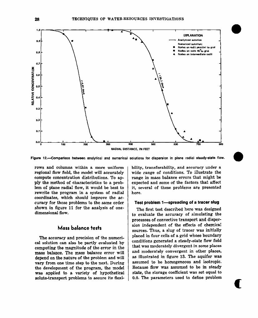
28 TECHNIQUES OF WATER-RESOURCES INVESTIGATIONS
0.9 -
0.8 -
EXPLANATION - Analytical solutim
Numerical solution: 0 Nodes on radii parallel to *id n Nodes cm radii 45% grid A Nodes on intermediate radii
0.2 -
0.1 -
0 100 200 300 400 800 500 700 800
RADIAL DISTANCE, IN FEET
Figure 12.-Comparison between analytical and numerical solutions for dispersion in plane radial steady-state flow.
rows and columns within a more uniform regional flow field, the model will accurately compute concentration distributions. To ap- ply the method of characteristics to a prob- lem of plane radial flow, it would be best to rewrite the program in a system of radial coordinates, which should improve the ac- curacy for those problems to the same order shown in figure 11 for the analysis of one- dimensional flow.
Mass balance tests
The accuracy and precision of the numeri- cal solution can also be partly evaluated by computing the magnitude of the error in the mass balance. The mass balance error will depend on the nature of the problem and will vary from one time step to the next. During the development of the program, the model was applied to a variety of hypothetical solute-transport problems to assure its flexi-
bility, transferability, and accuracy under a wide range of conditions. To illustrate the range in mass balance errors that might be expected and some of the factors that affect it, several of these problems are presented here.
lest problem l-spreading of a tracer slug
The first test described here was designed to evaluate the accuracy of simulating the processes of convective transport and disper- sion independent of the effects of chemical sources. Thus, a slug of tracer was initially placed in four cells of a grid whose boundary conditions generated a steady-state flow field that was moderately divergent in some places and moderately convergent in other places, as illustrated in figure 13. The aquifer was assumed to be homogeneous and isotropic. Because flow was assumed to be in steady state, the storage coefficient was set equal to 0.0. The parameters used to define problem c

MODEL OF SOLUTE TRANSPORT IN GROUND WATER 29
EXPLANATION
m No-flow boundary
Constant- head boundary
1+‘+1 Initial concentration (Co) equals
100: elsewhere Co=0
-9O- Computed potenticmetric altitude. Contour interval 2.0 feet (0.61 meter)
AX= 900 feet (274 meters)
Au= 900 feet (274 meters)
Figure 13.-Grid, boundary conditions, and flow field for test problem 1.
1 are listed in table 2. The slug of known mass was then allowed to spread down- gradient for a period of 2.0 years.
Table P.-Model parameters for test problem 1
Aquifer properties Numerical Darametera
Kz0.006 ft/s Ax=!?00 ft (1.6xlO-3 m/s) (274 m)
bz20.0 ft Ay=SOO ft (6.1 m) (274 m)
szo.0 CELDISz0.49 ez0.30 NPTPND=S
ar/aL=0.30
The model first computed a steady-state head distribution, shown in figure 13, and velocity field. The model required 12 time increments (or particle movements) to simu- late a 2.0-year period. The model was run to simulate conditions of no dispersion (aL = 0.0 ft) as well as moderate dispersion (aL = 100 ft or 30.6 m). The mass balance error com- puted using equation 64 is shown in figure
14 for both conditions. In these tests the error averages 1.9 percent and is always within a range of +8 percent. Much of the error is related to the calculation of nodal concentrations based on the arithmetic mean of particle concentrations in each cell. When a particle moves across a cell boundary, its area of influence shifts entirely from the first node to the second. Thus, depending on the local density of points and local concentra- tion gradients, the use of an arithmetic mean to compute nodal concentrations may give too much weight to some particles and too little weight to others. The use of a weighted mean, in which the weighting factor is a function of the distance between a node and a particle, reduced the error to some degree. But the improvement in precision was small compared with the increase in computational requirements, so this algorithm was not in- cluded in the general program. Because the error caused by using an arithmetic mean is not cumulative, it is not considered a serious

TECHNIQUES OF WATER-RESOURCES INVESTIGATIONS
0
TIME, IN YEARS
Figure 14.-Mass balance errors for test problem 1.
EXPLANATION
m No-f low boundary
m Constant -head boundary
8 Injection well
@ Withdrawal well
-9O- Computed potentiometric altitude. Contour interval 2.0 feet (0.61 meter)
A X= 900 feet (274 meters)
L\y= 900 feet (274 meters)
Figure lli.-Grid, boundary conditions, and flow field for test problem 2.

MODEL OF SOLUTE TRANSPORT IN GROUND WATER 31
problem. Furthermore, figure 14 shows that the error decreases for a higher dispersivity because dispersion smooths out sharp fronts and minimizes strong concentration gradients.
Test problem 2-effects of wells
The second problem was designed to eval- uate the application of the model to prob- lems in which the flow field is strongly in- fluenced by wells. The grid and boundary conditions used to define this problem are illustrated in figure 1.5. The problem con- sists of one injection well and one with- drawal well, whose effects are superimposed on a regional flow field controlled by two constant-head boundaries. The parameters for problem 2 are defmed in table 3. The aquifer was also assumed to be homogeneous and isotropic. The model simulated a period of 2.4 years and assumed steady-state t-low.
The model required 18 time increments (or particle movements) to simulate a 2.4- year period of solute transport. Problem 2 was also evaluated for conditions of no dis- persion (,,=O.O ft) as well as moderate dis- persion (at= 100 ft or 30.5 m) . The mass bal- ance error was computed using equation 62 and is shown in figure 16 for both conditions. The average of the 36 values shown in figure 16 is -0.06 percent ; the error always falls within the range of 2-8 percent. It can be
Table 3.-Model parameters for test problems 2 and 3
Aquifer properties and stresses Numerical parameters
Kz0.005 ft/s Ax=900 ft (1.5x1O-s m/s) (274 m)
bz20.0 ft Ay =QOO ft (6.1 m) (274 m)
s=o.o CELDIS ~0.50 ez0.30 NPTPNDz9
ar/aL=0.30 c’=lOO.O CGO.0 qwz1.0 fV/s
(0.028 ma/s)
seen that in this case the errors are essen- tially coincident for almost 1 year, after which the error appears to be dependent on the magnitude of dispersion. However, the model output showed that when aL= 100 ft (30.5 m) , the leading edge of the break- through curve (or chemical front) reaches the constant-head sink just prior to 1.0 year. When aL= 0.0 ft, the leading edge of the breakthrough curve still had not entered the constant-head sink after 2.4 years. Because the two curves in figure 16 are essentially coincident prior to 1.0 year, it thus appears that the divergence of the two curves is not caused directly by the difference in disper- sivity. Rather, it is related to the difference in arrival times at the hydraulic sinks and is a direct effect of the manner in which con-
TIME, IN YEARS
Figure 16.-Mass balance errors for test problem 2.
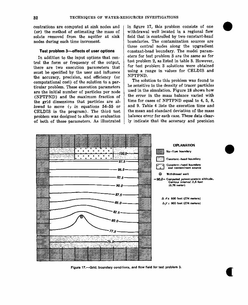
32 TECHNIQUES OF WATER-RESOURCES INVESTIGATIONS
centrations are computed at sink nodes and (or) the method of estimating the mass of solute removed from the aquifer at sink nodes during each time increment.
Test problem 3-effects of user options In addition to the input options that con-
trol the form or frequency of the output, there are two execution parameters that must be specified by the user and influence the accuracy, precision, and efficiency (or computational cost) of the solution to a par- ticular problem. These execution parameters are the initial number of particles per node (NPTPND) and the maximum fraction of the grid dimensions that particles are al- lowed to move (7 in equations 54-55 or CELDIS in the program). The third test problem was designed to allow an evaluation of both of these parameters. As illustrated
in figure 17, this problem consists of one withdrawal well located in a regional flow field that is controlled by two constant-head boundaries. The contamination sources are three central nodes along the upgradient constant-head boundary. The model param- eters for test problem 3 are the same as for test problem 2, as listed in table 3. However, f’or test problem 3 solutions were obtained using a range in values for CELDIS and NPTPND.
The solution to this problem was found to be sensitive to the density of tracer particles used in the simulation. Figure 18 shows how the error in the mass balance varied with time for cases of NPTPND equal to 4, 5, 8, and 9. Table 4 lists the execution time and the mean and standard deviation of the mass balance error for each case. These data clear- ly indicate that the accuracy and precision
EXPLANATION
m No-flow boundary
@ Withdrawal well
-w.O- Computed potantiometric altitude. Contour interval 2.5 feet (0.75 meter)
A X= SO0 feet (274 meters)
Ay = SW feet (274 meters)
Figure 17.-Grid, boundary conditions, and flow field for test problem 3.
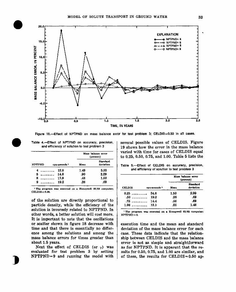
MODEL OF SOLUTE TRANSPORT IN GROUND WATER 33
EXPLANATION - NPTPNO: 4 O------o NPTPND: 5 A-- -A NPTPND- 8 O.......O NPTPND’ 9
0.0 0.5 1.0 1.5 2.0 2.5
TIME, IN YEARS
Figure 18.-Effect of NPTPND on mass balance error for test problem 3; CELDkk0.50 in all cases.
Table 4.-Effect of NPTPND on accuracy, precision, and efficiency of solution to test problem 3
NPTPND CDU-SH2Xld8 1
Mass balance error (percent)
Stalldard Mean deviation
4 ____-___ 12.8 1.49 5.33 5 -------- 14.0 .90 2.29 8 ________ 17.9 .48 1.53 9 -------- 19.2 .26 .69
1 The program was executed on a Honeywell 60/66 computer: CELDIS = 0.M).
of the solution are directly proportional to particle density, while the efficiency of the solution is inversely related to NPTPND. In other words, a better solution will cost more. It is important to note that the oscillations or scatter shown in figure 18 decrease with time and that there is essentially no differ- ence among the solutions and among the mass balance errors for times greater than about 1.6 years.
Next the effect of CELDIS (or 7) was evaluated for test problem 3 by setting NPTPND =S and running the model with
several possible values of CELDIS. Figure 19 shows how the error in the mass balance varied with time for cases of CELDIS equal to 0.25, 0.50, 0.75, and 1.00. Table 5 lists the
Table B.-Effect of CELDIS on accuracy, precision, and efficiency of solution to test problem 3
Masa bdance error (percent)
Standard CELDIS CPU-nda 1 Mean derfrtion
0.25 _________ 34.6 1.50 ii.99 .50 --------- 19.2 .26 .69 .75 ------___ 14.4 .56 .69
1.00 --------- 12.1 .25 1.48
1 The program was executed on * Honeywell 60/68 computer; NPTPND=Q.
execution time and the mean and standard deviation of the mass balance error for each case. These data indicate that the relation- ship between CELDIS and the mass balance error is not as simple and straightforward as for NPTPND. It is apparent that the re- sults for 0.50, 0.75, and 1.00 are similar, and of these, the results for ‘CELDIS= 0.60 ap

34 TECHNIQUES OF WATER-RESODRCES INVESTIGATIONS
-10.0 0.0 0.6 1.0 1.5 2.0 2.5
TIME, IN YEARS
Figure lg.-Effect of CELDIS on mass balance error for test problem 3; NPTPNDz9 in all cases.
pear to be the best. However, when CELDIS was reduced to 0.25, the error oscillated strongly for about 1.5 years before apparent- ly converging to a small error within the range of the other curves. This oscillation occurred because the maximum distance a particle could move (25 percent of the grid dimensions) was less than the spacing be- tween particles (33 percent of the grid di- mensions for NPTPND =9). Thus, convec- tive transport across the boundaries of cells could not be adequately represented for any single time step in those parts of the grid where the concentration was changing sig- nificantly with time. But over two successive time increments the error would average out to a minimum. As the contaminated area in- creases in size over time, the error in com- puted concentrations at cells near the front (that is, in areas of steep concentration gradient) becomes an increasingly smaller percentage of the total mass of solute present in the aquifer. Hence, the mass balance error generally tends to approach a minimal range with time for these types of problems.
The effects of NPTPND and CELDIS on the mass balance error are problem depend- ent. In problems for which CELDIS is not
the limiting stability criterion, varying CELDIS will have no effect on the solution. Because of the possible tradeoff between ac- curacy and efficiency, it is recommended in general that the model user specify NPTPND as 4 or 5 and CELDIS as 0.75 to 1.0 for runs made during the early stages of model calibration when frequent runs are made and maximum efficiency is desired. For final runs when maximum accuracy is de- sired, set NPTPND equal to 9 and CELDIS equal to 0.50.
Possible program modifications
The program presented here represents a basic and general solute-transport model. Some program modifications may be desir- able or even necessary to allow the model to be applied efficiently to a particular field problem. Some changes might require only minor adjustments, while others might in- volve major rewriting of the program. The purpose of this section is to discuss some of the modifications that might commonly be considered, and that might be incorporated into the present basic model, rather than us- ing an entirely different solution technique. c

MODEL OF SOLUTE TRANSPORT IN GROUND WATER 36
Coordinate system and boundary conditions
After the finite-difference grid is designed, the first program modification that should be made is to modify the array dimensions for the specific grid used. This will permit the most efficient use of computer storage. The array sizes should be set equal to NX, NY, and NPMAX, which are specified on Input Card 2. The maximum number of particles, NPMAX, may be computed from the follow- ing equation : NPMAX= (NX-2) (NY-2) (NPTPND)
where + (N,) (NPTPND) +250 (71)
N, is the number of nodes that repre- sent fluid sources, either at wells or at constant-head cells.
The values of NX and NY should be substi- tuted for the 20-by-20 arrays contained in COMMON statements PRMK, HEDA, HEDB, CHMA, CHMC, and DIFUS, and in DIMENSION statements on lines C170, G200, H140, and 1160. The value of NPMAX
0 should replace 3200 in the PART array in all the CHMA COMMON statements.
Although this program is designed for ap- plication to two-dimensional area1 flow prob- lems, it can be applied directly to two-di- mensional cross sections. In this case the x- coordinate would replace the y-coordinate. Then the user would have to assume and specify unit width (THCK array) for Ay and substitute hydraulic conductivity for transmissivity in data set 3 of attachment‘ III. If the problem ,involves transient flow, then specific storage (S’,) should be substi- tuted for the storage coefficient. Also, if re- charge or discharge is to be specified through the RECH array (data set 5)) values should be divided by the thickness of the layer (Ax)
to reduce the dimensionality of the stress rate to (T-l) rather than (LT-I) as indi- cated in the documentation. In applying the cross-sectional model to a field problem it is important that conditions meet the inherent assumption that there exist no significant components of flow into or out of the plane of the section. Because this assumption would probably be impossible to meet in the
vicinity of a pumping well, the use of the REC array (data set 2) should usually be limited to representing special or known-flux boundary conditions.
The program can also be applied directly and simply to one-dimensional problems. In this case one of the dimensions (NX or NY) should be reduced to a value of 3, of which the outer two are used to represent the no- flow boundaries around the one-dimensional row or column.
The most complex type of change would involve rewriting the program for applica- tion to other than a two-dimensional rectan- gular grid. One possibility includes problems of flow to or from wells in which radial symmetry can be assumed. This would allow variables to be expressed in terms of r-z co- ordinates. Another possibility is to simulate three-dimensional flow in x-y-x coordinates. A three-dimensional finite-difference flow model is available (Trescott, 1975) and would be compatible with the method-of-character- istics solution to the solute-transport equa- tion.
It is sometimes convenient to separately associate certain parts of the grid or certain boundary conditions with corresponding field conditions or hydrologic units. The analysis of flow patterns and water-quality changes may then be aided by performing separate mass balances (or budgets) for each char- acteristic type of node. The nodal types or zones can be conveniently identified through the NODEID array. Then the mass balance routines in subroutines CNCON and (or) OUTPT would have to be modified to tally fluxes separately for each NODEID ; for an example, see Konikow (1977). Similarly, if a coupled stream-aquifer system is being considered, a separate subroutine may be added to route streamflow downstream and progressively account for ground-water gains and losses and for tributary inflow or diversions. An example of such a modifica- tion is discussed by Konikow and Bredehoeft (1974).
For certain types of problems it may be desirable to be able to specify a constant- concentration boundary condition. The pro-

36 TECHNIQUES OF WATER-RESOURCES INVESTIGATIONS
gram could be modified to allow this by using a predetermined value or range in values of NODEID to identify this type of boundary. Then a statement could be added between lines G1090 and GllOO to reset the concen- tration at the node equal to the constant con- centration where this condition is specified. The value of the constant concentration can be stored in the CNRECH array. Note that the mass balance \calculation as presently written will not account for the mass of solute added or removed at a constant-con- centration boundary.
between the solutions to the flow and solute- a
Basic equations The basic equations that are solved by this
model were derived under a number of limit- ing assumptions. Some of these assumptions can be overcome through modificai;ions of the basic equations and corresponding changes in the program.
The program assumes that molecular dif- fusion is negligible. But if it is necessary to consider the process of molecular diffusion in a particular problem, the coefficient of hy- drodynamic dispersion (O+) can be redefined as the sum of the coefficient, of mechanical dispersion, which is defined by the right side of equation 5, and a coefficient of molecular diffusion. The consequent program modifica- tion would have to be made only in sub- routine VELO (lines E1280-E1680).
The solute-transport equation can also be modified to include the effects of first-order chemical reactions, as was done by Robert- son (1974). The reaction term could be in- cluded in the right side of equation 39. The corresponding program modification would be required in subroutine CNCON.
In certain problems the range in concen- trations may be so great that the dependence of fluid properties, such as density and vis- cosity, on the concentration may have to be considered because of the dependence of fluid flow on variations in fluid properties. In this case the flow equation (eq 1) would have to be rewritten in terms of fluid pressure, rather than hydraulic head, such as equation 16 of Bredehoeft and Pinder (1973, p. 197). Then the program can be modified to iterate
- transport equations if the change in fluid properties at any node exceeds some criterion during one time increment.
The flow equation can also be modified for a:pplication to unconfined aquifers in which the saturated thickness is a direct function of water-table elevation. This would require the inclusion of steps in subroutine ITERAT to correct the transmissivity for changes in saturated thickness. Such a feature is in- cluded in the two-dimensional flow model documented by Trescott, Pinder, and Larson (1976).
Input and output
The input and output formats have been designed for flexibility of use and general compatibility with the analysis of a variety of types of flow problems. If any of the for- mats are not suitable for use with a par- ticular problem, they should be modified ac- cordingly. All input formats are described in attachment III and contained in sub- routine PARLOD in the program.
It has been assumed that several aquifer parameters are constant and uniform in space, such as storage coefficient, effective porosity, and dispersivity. If any of these are known to vary in space, they should be re- defined as two-dimensional arrays. Then statements to allow these arrays to be read into the program should be added to sub- routine PARLOD. Similarly, values of leak- ante and source concentrations (CNRECH) are only read in data set 7, where values can be associated only with a limited number of unique node identification codes. If the varia- tions of these parameters are known on a more detailed scale, then they too can be read as additional data sets by adding appropriate statements to subroutine PARLOD. For ex- ample, a typical sequence of statements for reading one data set is represented by lines B2650-B2750, where the initial water-table elevations (data set 8) are read. This se- quence of statements can then be replicated for reading in a different data set and in- serted into subroutine PARLOD:
c

MODEL OF SOLUTE TRANSPORT IN GROUND WATER 37
A labeled listing of the input data deck for test problem 3 is provided in attachment IV. This example illustrates the use of the data input formats specified in attachment III and shows that only a few data cards are re- quired by the model to simulate a relatively simple problem. This example will also allow the user to verify that his program deck and computer yield essentially the same results as obtained by the documented program. Thus, selected parts of the output for test problem 3 are included in attachment V. Not all of the printed output from test problem 3 has been duplicated in attachment III. In- stead, it contains only a sufficient selection to illustrate the type and form of output pro- vided by the model, as well as to allow the user to compare his calculated values of cri- tical parameters, such as head, velocity, and concentration, with the values computed by the documented model.
Conclusions
The model presented in this report can simulate the two-dimensional transport and dispersion of a nonreactive solute in either steady-state or transient ground-water flow. The program is general and flexible in that it can be readily and directly applied to a wide range of types of problems, as defined by aquifer properties, boundary conditions, and stresses. However, some program modi- fications may be required for application to specialized problems or conditions not in- cluded in the general model.
The accuracy of the numerical results can be evaluated by comparison with analytical solutions only for relatively simple and ideal- ized problems ; in these cases there was good agreement between the numerical and analy- tical results. Mass balance tests also help to evaluate the accuracy and precision of the model results. The error in the mass balance is generally less than 10 percent. The range in mass balance errors is commonly the greatest during the first few time incre- ments, but tends to decrease and stabilize with time. For some problems the accuracy
and precision of the numerical results may be sensitive to the initial number of particles placed in each cell and to the size of the time increments, as determined by the stability criteria for the solute-transport equation. The results of several numerical experiments suggest that the accuracy and precision of the results are essentially independent of the magnitude of the dispersion coefficient, and comparable accuracies are attained for high, low, or zero dispersivities.
References Cited Aris, Rutherford, 1962, Vectors, tensors, and the
basic equations of fluid mechanics: Englewood Cliffs, N. J., Prentice-Hall, 286 p.
Bear, Jacob, 1972, Dynamics of fluids in porous media: New York, Am. Elsevier Publishing Co., 764 p.
Bredehoeft, J. D., and Pinder, G. F., 1973, Mass transport in flowing groundwater: Water Re- sources Research, v. 9, no. 1, p. 194-210.
Garder, A. O., Peaceman, D. W., and Pozzi, A. L., Jr., 1964, Numerical calculation of multidimen- sional miscible displacement by the method of characteristics : Sot. Petroleum Engineers Jour., v. 4, no. 1, p. 2686.
Konikow, L. F., 1977, Modeling chloride movement in the alluvial aquifer at the Rocky Mountain Arsenal, Colorado: U.S. Geol. Survey Water- Supply Paper 2044, 43 p.
Konikow, L. F., and Bredehoeft, J. D., 1974, Model- ing flow and chemical quality changes in an irrigated stream-aquifer system: Water Re- sources Research, v. 10, no. 3, p. 646-662.
Konikow, L. F., and Grove, D. B., 1977, Derivation of equations describing solute transport in ground water: U.S. Geol. Survey Water-Re- sources Investigatons 77-19, 30 p.
Lohman, S. W., 1972, Ground-water hydraulics: U.S. Geol. Survey Prof. Paper 708, 70 p.
Pinder, G. F., and Bredehoeft, J. D., 1968, Applica- tion of the digital computer for aquifer evalua- tion: Water Resources Research, v. 4, no. 6, p. 1069-1093.
Pinder, G. F., and Cooper, II. II., Jr., 1970, A nu- merical technique for calculating the transient position of the saltwater front: Water Re- sources Research, v. 6, no. 3, p. 876-882
Prickett, T. A., and Lonnquist, C. G., 1971, Selected digital computer techniques for groundwater re- source evaluation: Illinois Water Survey Bull. 66, 62 p.

38 TECHNIQUES OF WATER-RESOURCES INVESTIGATIONS
Reddell, D. L., and Sunada, D. K., 1970, Numerical simulation of dispersion in groundwater aqui- fers: Colorado State Univ. Hydrology Paper 41, 79 p.
Robertson, J. B., 1974, Digital modeling of radio- active and chemical waste transport in the Snake River Plain aquifer at the National Re- actor Testing Station, Idaho: U.S. Geol. Survey Open-File Rept. IDO-22064, 41 p.
Robson, S. G., 1974, Feasibility of digital water- quality modeling illustrated by application at Barstow, California: U.S. Geol. Survey Water- Resources Investigations 46-73, 66 p.
Scheidegger, A. E., 1961, General theory of disper- sion in porous media: Jour. Geophys. Research, v. 66, no. 10, p. 3273-3278.
Trescott, P. C., 1975, Documentation of finite-dif- ference model for simulation of three-dimen- sional ground-water flow: U.S. Geol. Survey Open-File Rept. 75-438, 32 p.
Trescott, P. C., Pinder, G. F., and Larson, S. P., 1976, Finite-difference model for aquifer simu- lation in two dimensions with results of numeri- cal experiments: U.S. Geol. Survey Techniques of Water-Resources Investigations, Book 7, Chap. Cl, 116 p.
von Rosenberg, D. U., 1969, Methods for the nu- merical solution of partial differential equa- tions: New York, Am. Elsevier Publishing Co., 128 p.
c

COAAPUTER PROGRAM AND RELATED DATA

C C
0 C C C
C
C
C
C C
MODEL OF SOLUTE .TRANSPORT IN GROUND WATER
Attachment I FORTRAN IV Program Listing
*****************************~********************************** l l
l SoLuTE TRANSPORT AND DISPERSION IN A POROUS F~EDIUM 4 4 NUMERICAL SOLUTION --- METHOD OF CHARACTERISTICS l
* PROGRANMED BY J. 0. BREDEHOEFT AND L. F. KONIKOW l
4 4
**********C*******t*********************************************
DOUELE PRECISION DMINl,DEXP,DLOG,DABS REAL *8TMRX,VPRM,HIrHR,HC,HK,~T,RECIRECH,TIH,AOPT,TITLE REAL *8XDEL,YDEL,S,AREA,SUMT,RHO,PARAM,TEST,TOL,PINT,HMIN,PYR REAL l 8TINT,ALPHAl ,ANITP COMMON /PRMI/ NTIM,NPHP,NPNT,NITP,N,NX,NY,NP,NREC,INT,NNX,NNY,NU~O
~B~,N~~~,I~~V,N~~AX,IT~AX,N~~RIT,I~RNT,N~T~N~,N~NT~~,N~NT~L,~~NTD,N ZPNCHV,NPDELC
COMMON /PRMK/ NODEID~2O,2O~rNPCELL~2~,2~~,LIMBO~~~O~,IXOBS~3~,IYOB lS(5)
COMMON /HEDA/ THCK~20,2O~,PERM~2O,2O~,TMUL~~,~O~.TMOBS~~O~,ANFCTR COMMON /HEDB/ TMRX~20,20,2~,VPR~~20,20~,H1~20,20~,HR~20,20~,HC~20,
120~,HK~20.20~,WT~20.20~,REC~20,20~,RECH~20,20~,T1M~100~,A0PT~20~,1 2ITLE~lOl,XDEL,YDEL,S,AREA,SU~T,RHO,PARAH,TEST,TOL,PINT,H~IN,PYR
COMMON /CHMA/ PART~3,3200~,C0NC~20,20~,THCN~S,~0~,VX~20,20~,VY~20, 12O~,CONINT~2O,2O~,CNRECH~2O,2O~,POROS,SUHTCH,~ETA,TIHV,STORM,STORM 2I,C~SIN,C~SOUT,FLMIN,FLMOT,SUMIO,CELDIS,DLTRAT,CSTORH
*************************************************************** ---LOAD DATA---
INT=O CALL PARLOD CALL GENPT *************************************************************** ---START COMPUTATIONS---
---COMPUTE ONE PUMPING PERIOD--- DO 150 INT-1rNPHP IF (INT.GT.l) CALL PARLOD
---COMPUTE ONE TIME STEP--- DO 130 N=l .NTIM IPRNT=O
---LOAD NEW DELTA T--- TINT=SUMT-PYR*(INT-1) TDEL=Dl4INl(TIM(N),PYR-TINT) SUMT=SUMT+TDEL TIM(N) =TDEL REHN=MOD(N.NPNT) *************************************************************** CALL I TERAT IF (REMN.EQ.O.O.OR.N.EQ.NTIM) CALL OUTPT CALL VELO CALL flOVE **f************************************************************
---STORE OBS. WELL DATA FOR TRANSIENT FLOU PROBLEMS--- IF (S.EQ.o.0) GO TO 120 IF (NUMOBS.LE.0) GO TO 120 J=MOD( N,SO) IF (J.EQ.0) J’s0 TMOBS( J)=SUMT DO 110 I=l,NUWOBS TMUL(I,J)=HK(IXOBS(I)rlYOBSO) TMCN<I,J)=CONC(IXOBS(J)rIVOBS(I))
3 110 CONTINUE
41
A 10 A 20 A 30 A 40 A so A A ti A 80 : 100 90
A 110 A 120 A 130 A 140 A 150 A 160 A 170 A 180 A 190 A 200 A 210 A 220 A 230 A 240 A 250 A 260 A 270 A 280 A 290 A 300 A 310 A 320 A 330 A 340 A 350 A 360 A 370 A 380 A 390 A 400 A 410 A 420 A 430 A 440 A 450 A 460 A 470 A 480 A 490 A 500 A 510 A 520 A 530 A 540 A 550 A 560 A 570 A 580

42 TECHNIQUES OF WATER-RESOURCES INYESTIGATIONS
FORTRAN IV program htting-Continued
C *************************************************************** C ---OUTPUT ROUTINES---
120 IF CREMN.EQ.0.0.OR.N.EQ.NTIH.OR.MOD(N,SO).EQ.0~ CALL CHMOT IF CSUMT.GE.CPYR*INTI) GO TO 140
130 CONTINUE C *************************************************************** C ---SUHRARY OUTPUT---
140 CONTINUE IPRNT=l CALL CHMOT
150 CONTINUE C ***************************************************************
STOP C ***************************************************************
END SUBROUTINE PARLOD DOUBLE PRECISION DMINl l DEXPIDLOGIDABS REAL *8THRX~VPRNrHI,HR~HC,HK~UT~REC~RECH,TIN,AOPT,TITLE REAL *~XDELIYDEL~SIAREAISUMTIRHOIPARA~~TESTITOL,PINT,HMIN,PYR REAL l 8FCTR~TIMX~TINIT~PIESIYNSIXNSIRATIHMX,HMX~HMY REAL l 8TINT#ALPHAlrANITP CONMON /PRHI/ NTIHrNPMP~NPNT~NITP~N~NX~NY~NP~NREC~INT~NNX~NNY~NUMO
~~S.NMOV,IHOVINPMAXIITMAX~N~CRIT~IPRNT~NPTPND,NPNTMV,NPNTVL,NPNTD,N 2PNCHVeNPDELC
COMMON /PRMK/ NODEID~20~20~rNPCELL~20~2O~,LIHBO~S0O~,IXOBS~3~~IYO~ lSC5)
COMRON /HEDA/ THCK~20~20~rPERH~20~20~~THUL~S,S0~~TMOBSC~O~.ANfCTR COMMON /HEDB/ TMRX(~~I~~I~)~VPRM(~OIZO)~HI(~~,~~)~HR(~~~~~)~HC(~~~
~~~)~HKC~~I~~)~WT(~~IZO)~REC(~~~~~~,RECH~~~,~O~,TIM~~~~~,AOPT~~~~,T 2ITLE~lO~rXDEL,YDEL,SIAREAISUMTIRHOIPARAM,TEST,TOL~PINT,HMIN,PYR
COMMON /CHHA/ PART~3,3200~,C0~C~20,20~,TMCN~5,50~,VX~20,20~,VY~20. 120~rCONINT~20,20~rCNRECH~20,20~.POROS~SUMTCH,~ETA~TIMV~STORM~STORM ~I~CHSIN~CMSOUT.FLMIN.FLMOT.SUMIO.CELDIS.DLTRAT.CSTORM
CONMON /BALM/ TOTLP COMMON /XINV/ DXINVIDYINVIARINVIPORINV COMMON /CHMC/ SUMCC~~I~~),VXBDYC~~IZO)~VYBDY(ZOIZO)
C *************************************************************** IF CINT.GT.1) GO TO 10 WRITE (6,750) READ (5,720) TITLE WRITE (6r730) TITLE
C *************************************************************** C ---INITIALIZE TEST AND CONTROL VARIABLES---
STORMI=0.0 TEST=0.0 TOTLQ=O.O SUHT-0 .O SUMTCHMO.0 INT-0 IPRNT=O NCA=O N=O 1r4ov=o NHOV=O
C *************************************************************** C ---LOAD CONTROL PARAMETERS---
READ (5.740) NTIH,NPMPINXINYINPWAXINPNTINI~PINUMOBSIITMAX~NREC~NPT ~PND,NCODESINPNTMVINPNTVLINPNTOINPDELC,NPNCHV
READ (3,800) PINTITOLIPOROSIBETAISIT~~X,TIN~~~XDELIVDEL~DLTRAT~CEL lDIS#ANFCTR
PYR=PINT*86400.0*365.25 NNX=NX -1
A 590 A 600 A 610 A 620 A 630 A 640 A 650 A 660 A 670 A 680 A 690 A 700 A 710 A 720 A 730- 8 10 9 20 8 30 B 40 B 50 8 60 8 70 B 80 B 90 B 100 B 110 8 120 a 130 a 140 0 150 B 160 0 170 B 180 B 190 B 200 B 210 8 220 8 230 B 240 B 250 0 260 B 270 0 280 B 290 B 300 8 310 B 320 B 330 B 340 B 350 8 360 8 370 0 380 B 390 B 400 0 410 EI 420 8 430 0 440 B 450 0 460 0 470
c

MODEL OF SOLUTE TRANSPORT IN GROUND WATER 43
FORTRAN IV program listing--Continued
NNY=NY-1 B 480 NP=NPMAX B 490 OXINV=l.O/XDEL B 500 DYINV=l .O/YDEL B 510 ARINV=DXINV+DYINV B 520 PORINVfl.O/POROS 0 530
C ---PRINT CONTROL PARAMETERS--- WRITE C6r760)
0 540 B 550
WRITE (68770) NXINYIXDELIYDEL B 560 WRITE C6r780) NTIMINPMPIPINTITIMXITINIT B 570 WRITE C6r790) SIPOROSIBETAIDLTRATIANFCTR 0 580 WRITE (68870) NITPITOLIITMAXICELDISINPMAXINPTPND B 590 IF (NPTPND.LT.G.OR.NPTPND.GT.9.OR.NPTPND.EQ.6.OR.NPTPND.EQ.7~ WRIT 8 600
1E C6r880) t3 610 WRITE C6r890) NPNT,NPNTMVINPNTVL,NPNTD,NUMOBSINRECINCODES~NPNCHV~N B 620
1PDELC B 630 IF CNPNTMV.EQ.0) NPNTMV=999 B 640 GO TO 20 0 650
C **+tt****+i**tt+**2t~~~*~~*~n*~~.~,.*.~*~~..~~~~~~~~~~~~.~~...~ B 660 C ---READ DATA TO REVISE TIME STEPS AND STRESSES FOR SUBSEQUENT B 670 C PUMPING PERIODS--- e 680
10 READ C5#1060) ICHK e 690 IF CICHK.LE.0) RETURN B 700 READ (5r1070) NTIM,NPNTINITPIITMAXINREC,NPNT~VINPNTHV~NPNTVL~NPNT~~NPDELC i3 710
I~NPNCHVIPINT,TIMXITINIT B 720 WRITE (6r1080) INT B 730 WRITE CbrlC90) NTIM,NPNTINITPIITMAX.NREC.NPNTMV~NPNTVL~NPNTD~NP~EL 0 740
~CINPNCHVIPINTITIMXITINIT C ****t*ttt***tt*tt*tt~.~*~***Ct****~~.~~~~~~.~~~~~.~~~~~~~
C ---LIST TIME INCREMENTS--- 20 DO 30 J=lrlOO
TIM(J) =O.O 30 CONTINUE
TIM(l) =TINIT IF CS.EQ.O.0) GO TO 50 DO 40 K=Z,NTIM
40 TI?4CK)=TIMX*TIMCK-1) WRITE (6~470) WRITE (6r490) TIM GO TO 60
50 TIMCl)=PYR WRITE (6r480) TIM(l)
C t**t*****t~****t***tt*****t**tt**t**tt**~~~**~~~~~~~~~~~~~.~.~~ C ---INITIALIZE MATRICES---
60 IF CINT.GT.l) GO TO 100 DO 70 IY=1,NY DO 70 IX=l,NX VPRMCIXt1Y)‘O.O PERM(IXeIY)=O.O THCK(IXIIY)=O.O RECH(IXIIY)=O.O CNRECH(IXIIY)=O.O REC(IX,IY)=O.Cl NODEIO(IXIIY)=O TMRX(IXIIY,~)=O.O TMRX(IX,IY,Z)=O.O HI(IX,IY)=O.O HR(IXpIY)=O.O HC(IX,IY)=O.C HK(IX,IY)=O.O WT(IXIIY)=CI.O vx(Ix~IY)=o.o
0 750 B 760 B 770 B 780 B 790 0 800 B 810 8 820 0 830 B 840 B 850 0 860 B 870 0 880 B 890 0 900 B 910 0 920 B 930 B 940 B 950 B 960 0 970 B 980 B 990 81000 81010 I31020 81030 81040 810’30 01060 81070 81080 81090

44 TECHNIQUES OF WATER-RESOURCES INVESTIGATIONS
FORTRAN IV program listing-Continued
vY(Ix~IY)=o.o a1100 VXBDYCIX,IY)=O.O IT1110 VYBDY(IX,IY)=O.O Bll20 CONCCIX.IY)=0.0 81130 CONINTCIX,IYI=0.0 81140 SUMcCIX,IY)=O.O 81150
70 CONTINUE Bll60 C ****************t************+******,~*************************** 81170 C ---READ OBSERVATION UELL LOCATIONS--- 01180
IF CNUMOBS.LE.0) GO TO 100 81190 WRITE C6r900I Bl200 DO 80 J=lr#UWOBS Bl210 READ (5,700)' IX,IY Bl220 WRITE (6r810) JIIXIIY 81230 IXOBS< J)=IX 81240
80 IYOBSCJI'IY Bl250 DO 90 I=lrNUMOBS 81260 DO 90 J=lrSO 81270 TMULCIrJ)=O.O El280
90 TMCNCIrJI=0.0 01290 C t***t***tt******t*************,********************************** 81300 C ---READ PUMPAGE DATA -- (X-Y COORDINATES AND RATE IN CFSI--- 01310 C ---SIGNS : YITHDRAYAL = POS.; INJECTION = NEG.--- 61320 C ---IF INJ. WELLI ALSO READ CONCENTRATION OF INJECTED UATER--- 81330
100 IF CNREC.LE.O) GO TO 120 81340 URITE (6,910) 81350 DO 110 I=lrNREC 81360 READ CSr710) IXIIYIFCTR~CNREC 81370 IF CFCTR.LT.O.O) CNRECHCIXIIY)=CNREC 81380 RECCIXIIYI'FCTR 81390
110 WRITE (6r8ZOI IX,IY,RECCIXIIYI~CNRECHCIX~IYI et31400 C **t*******t***************************************************** 81410
120 IF <INT.GT.l) RETURN 81420 AREA=XDEL*YDEL 81430 WRITE C6r690) AREA 81440 URITE C6r600) 81450 WRITE (6r610) XDEL 81460 URITE <6#610) YDEL 81470
C *****t*t*t*t**************************************************** 81480 C ---READ TRANSMISSIVITY IN FT**Z/SEC INTO VPRM ARRAY--- 81490 C ---FCTR = TRANSMISSIVITY MULTIPLIER M-S> FT**Z/SEC--- 81500
YRITE (6r530) 81510 READ CSr550) INPUTIFCTR 81520 DO 160 IY=lrNY 81.530 IF CINPUT.EQ.1) READ (5.560) CVPRMCIXIIY)~IX=~~NX) 81540 DO 150 IX'lrNX BlSSO IF CINPUT.NE.l) GO. TO 130 BlS60 VPRMCIXIIY)=VPRMCIXIIY)*FCTR 81570 GO TO 140 81580
130 VPRMCIXIIYIMFCTR 81590 140 IF CIX.EQ.l.OR.IX.EQ.NX) VPRWCIX.IY)=O.O 81600
IF CIY.EQ.l.OR.IY.EQ.NY) VPRHCIXIIY)=O.~ 81610 150 CONTINUE 81620 160 URITE (6,520) CVPRMCIXIIY)~IX=~~NX) 81630
C **************************************************************** 81640 C ---SET UP COEFFICIENT MATRIX --- BLOCK-CENTERED GRID--- 81650 C ---AVERAGE TRANSWISSIVITY --- HARMONIC MEAN--- 81660
IF CANFCTR.NE.O.O) GO TO 170 81670 URITE C6r1050) 81680 ANFCTRIl.0 81690
170 PIES=3.1415927*3.1415927/2.0 YNS=NY*NY
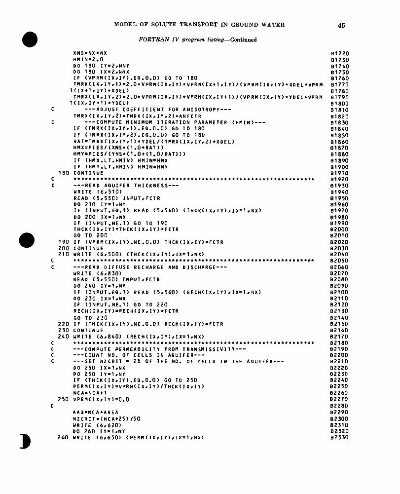
MODEL OF SOLUTE TRANSPORT IN GROUND WATER 45
FORTRAN IV program listing-Continued
XNS=NX l NX HMIN=2.0 DO 180 IY=~?INNY DO 180 IX=2,NNX IF CVPRMCIX~IY).EQ.O.O) GO TO 180 TflRX~IX~IY~l~=2.0*VPRM~IXIIY)*VPRM~IXtl~IY~/~vPRN~IX~IY~~xDELtvPRM
lCIXtlrIY)+XDEL) T~RX~IX~IY~2~=2.O+VPRM~IXIIY)+VPRM~IXIIrtl~/~VPRM~IX~IY~*YDELtVPRM
lCIX~IYtl)*YDEL) C ---ADJUST COEFFICIENT FOR ANISOTROPY---
TMRXCIXIIY,~)=TMRXCIXIIYIZ)~ANFCTR C ---COMPUTE HINIMU# ITERATION PARAMETER (HMIN)---
IF CTMRX(IXIIY,~).EQ.O.O) GO TO 180 IF (TMRX(IXIIYI~).EP.O.O~ GO TO 180 RAT=TMRXCIXIIYI~)+YDEL/(T~RX(IXIIY,~~*XDEL~ tiMX=PIES/CXNS*Cl.O*RAT)) HMY=PIES/CYNS*Cl.O*Cl.O/RAT))) IF CHMX.LT.HMIN) HMIN=HMX IF (HMY.LT.HMIN) HMIN=HMY
180 CONTINUE C ******.**,+tt***t*************t****+*+*2*..~~~~~.~.~~~~~~~~*~~~~ C ---READ AQUIFER THICKNESS---
URITE (6,510) READ C SrSSO) INPUT, FCTR DO 210 IY=lrNY IF CINPUT.EQ.1) READ (5,540) CTHCKCIXIIY),IX=~,NX) DO 200 IX=l,NX IF (1NPUT.NE.T) GO TO 190 THCKCIX.IY)=THCKCIX.IY)*FCTR GO TO 200
190 IF CVPRMCIXIIY).NE.~.O) THCKCIXIIY)=FCTR 200 CONTINUE 210 WRITE (6rSOO) CTHCKCIXIIY)~IX=~~NX)
C t*******tt+****+t***+*******tt**+tttt*+t*~~~~~~*~~*~~~~~~~~~~~~~ C ---READ DIFFUSE RECHARGE AND DISCHARGE---
WRITE (6,830). READ C SrSSO) INPUT,FCTR DO 240 IY=lrNY IF (1~puT.EQ.l) READ (5,560) CRECH(IX~IY)~IX=~~NX) DO 230 IX=lrNX IF CINPUT.NE.l) GO TO 220 RECHCIX,IY)=RECH(IXtIY)*FCTR GO TO 230
220 IF CTHCKCIXIIY).NE.O.O) RECHCIXeIY)=FCTR 230 CONTINUE 240 WRITE (6,840) CRECHCIXIIY)~IX=~~NX)
C t+tt+*+tt*.t**+tC***~~~~~~.~~~~*~~~**~~4~~**~*~*~~*~*~~*~~~4*~~*
: ---COMPUTE PERMEABILITY FROM TRANSHISSIVITY--- ---COUNT NO. OF CELLS IN AQUIFER---
C ---SET NZCRIT = 2% OF THE NO. OF CELLS IN THE AQUIFER--- DO 250 IX=lrNX DO 250 IY=l,NY IF (THCK(IX,IY).EQ.O.O) GO TO 250 PERM(IX,IY)=VPRM(IX~IY)/THCK~IX~IY~ NCA=NCAtl
2SO VPRM(IXIIY)=O.O L
AAQ=NCA*AREA NZCRIT=CNCAt2s)/s0 WRITE (6.620) DO 260 IY=lrNY
B
260 WRITE (6r650) (PERMCIXIIY)~IX=~~NX)
81720 81730 81740 81750 81760 81770 81780 81790 81800 81810 81820 81830 B1840 B18SO Bl860 81870 81880 81890 Bl900 B1910 01920 81930 81940 B19SO 81960 81970 B1980 81990 BZOOO B2010 B2020 82030 82040 82050 82060 82070 82080 B2090 B2100 B2110 B2120 B2130 82140 821 SO 82160 82170 B2180 B2190 B2200 B2210 B2220 82230 82240 B22S0 82260 82270 82280 B2290 82300 82310 82320 82330

TECHNIQUES OF WATER-RESOURCES INVESTIGATIONS
FORTRAN IV program listing-continued
WRITE (6,630) NCAIAAQINZCRIT C **t*********t***t*********************************************** C ---READ NODE IDENTIFICATION CARDS--- C ---SET VERT. PERM.# SOURCE C0NC.r AND DIFFUSE RECHARGE--- C ---SPECIFY CODES TO FIT YOUR NIEEDS---
WRITE (6r570) READ (5,550) INPUTIFCTR DO 280 IY=lrNY IF CINPUT.EQ.l) READ (5,640) CNODEIDCIX,IY),IX=l~NX) DO 270 IX’lrNX
270 IF CINPUT.NE.l.AND.THCK(IXIIY).NE.O.O) NODEIDCIXIIY)=FCTR 280 WRITE (6,580) CNODEIDCIX~IY)~IX=~~NX)
WRITE C6r920) NCODES IF CNCODES.LE.0) GO TO 310 WRITE (6~930) DO 300 IJ=l,NCODES READ (5,850) ICODEIFCTR~~FCTR~IFCTR~~OVERRD DO 290 IX=lrNX DO 290 IY=lrNY IF CNODEIOCIX~IY).NE.ICODE) GO TO 290 VPRMCIX,IY)=FCTRl CNRECHCIX,IY)=FCTRZ IF COVERRD.NE.O) RECHCIX,IY)=FCTR3
290 CONTINUE WRITE C6r860) ICODEIFCTR~~FCTR~
300 IF COVERRD.NE.O) WRITE (6rllOO) FCTR3 310 WRITE C6r590)
DO 320 IY=lrNY 320 WRITE C6rS20) CVPRMCIX~IY)~IX=~~NX)
C *t***+++*++****************************************~*****~***** C ---READ WATER-TABLE ELEVATION---
WRITE C6r670) READ C3rSS0) INPUTeFCTR DO 350 IY-1rNY IF CINPUT.EQ.l) READ CSr660) ~WTCIXIIY)~IX=~~NX) DO 340 IX-1rNX IF CINPUT.kE.1) GO TO 330 WTCIX~IY)=wTCIX~IY)*FCTR GO TO 340
330 IF CTHCKCIX,IY).NE.O.O) WTCIX,IY)=FCTR 340 CONTINUE 350 WRITE (6,680) CWTCIX,IY),IX=lrNX)
C +****************t.********************************************** C ---SET INITIAL HEADS---
DO 360 IX=lrNX DO 360 IY’lrNY HICIX,IY)=WTCIX.IY) HC(IX~IY)=HI(IXIIY) HRCIX~IY)‘=HICIXIIY)
360 HKCIX,IY)=HICIXIIY) C
CALL OUTPT C *+****+t*****t************************************************* C ---COMPUTE ITERATION PARAMETERS---
DO 370 ID=lr20 AOPTCID)=O.O
370 CONTINUE ANITP’NITP-1 ALPHAl=DEXPCDLOGCl .O/HMIN)/ANITP) AOPT(1 )=HMIN DO 380 IP=Z#NITP
380 AOPTCIP)=AOPTCIP-l)*ALPHAl
82340 82350 82360 82370 82380 82390 82400 82410 82420 82430 132440 82450 82460 02470 82480 I32490 B2SO0 82510 I32520 82530 82540 82550 132560 82570 82580 82590 02600 I32610 02620 02630 82640 82650 82660 82670 82680 82690 82700 82710 82720 82730 82740 82750 82760 82770 82780 82790 82800 62810 82820 82830 82840 82850 82860 82870 82880 82890 82900 02910 B2920 82930 82940 82950
c

MODEL OF’ SOLUTE TRANSPORT IN GROUND WATER
FORTRAN IV program listing-Continued
C
C C
390 400 410 420
C C
430
440 C
WRITE (6r450) WRITE (6r460) AOPT *****tt****t**************************************************** ---READ INITIAL CONCENTRATIONS AND COMPUTE INITIAL MASS STORED--- READ (5r550) INPUTIFCTR DO 420 IY=lrNY IF (1NPUT.EQ.l) READ (5,660) (CONC(IX~IYI,IX=l,NX) DO 410 IX-1rNX IF (INPUT.NE.l) GO TO 390 CONC(IX~IYI'CONC(IX~IY)*FCTR GO TO 400 IF (THCK(IX~IY).NE.O.OI CONC(IXIIY)=FCTR CONINT(IX~IY)=tONC(lXIIV) STORMl~STORMI+CONINT~IXIIr)*THCK~IX,IY~*AREA*POROS CONTINUE ****t*t*****t**t************************************************ ---CHECK DATA SETS FOR INTERNAL CONSISTENCY--- DO 440 IX=lrNX DO 440 IY'lrNY IF (THCK<IXIIYI.GT.O.O) GO TO 430 IF (TMRX(IX~IY~l).GT.o.oI WRITE (6r940) IXIIY IF (TMRX(lX~lY~2).GT.o.o) WRITE (6,950) IXIIY IF (NODEID(IX,IYI.GT.O) WRITE (6r960) IXIIY IF (WT(IX,IY).NE.O.O) WRITE (6,970) IXIIY IF (RECH(IXIIYI.NE.O.O) WRITE (6r980I IXIIY IF (REC(lX~IY).NE.o.o) WRITE (6r990) IX,IY IF (PERM(IX~IYI.GT.O.OI GO TO 440 IF (NODEID(IX,IYI.GT.O.O) WRITE (601000) IXIIY IF (WT(IX,IYI.NE.O.OI WRITE (6rlOlO) IXIIY IF (RECH(IX~IY).NE.O.O) WRITE (6,102oI IxIIY IF (REC(IX,IY).NE.O.OI WRITE (6r1030) IXIIY IF (THCK(IX,IY).GT.O.O) WRITE (6r1040) IXIIY CONTINUE ********t******************************************************* RETURN ***********tt***************************************************
a b
450 FORMAT (1Hlr2OHITERATION PARAMETERS) 460 FORMAT (3H rlG20.6) 470 FORMAT (lHlr27HTIflE INTERVALS (IN SECONDS)) 480 FORMAT (lHlrlSX,17HSTEADY-STATE FLOW//SX,57HTIME INTERVAL (IN SEC)
1 FOR SOLUTE-TRANSPORT SIMULATION = l G12.5) 490 FORMAT (3H r10G12.5) 500 FORMAT (3H r20~5.1) 510 FORMAT (lHlr22HAQUIFER THICKNESS (FT)) 520 FORMAT (3H r20F5.2) 530 FORMAT (lHlr3oHTRANSMISSIVITY MAP (FT*FT/SEC)) 540 FORMA? (2OG3.0) 550 FORMAT (IlrG10.0) 560 FORMAT (2OG4.1) 570 FORMAT (lHlr23HNODE IDENTIFICATION HAP//I 580 FORMAT (1H r2015) 590 FORMAT (lHlr45HVERTICAL PERMEABILITY/THICKNESS (FT/(FT*SEC))) 600 FORMAT (lH0,10X112HX-Y SPACING:) 610 FORMAT (1H rl2X.lOG12.5)~ 620 FORMAT (lHlr24HPERMEABILTY MAP (FT/SEC)) 630 FORMAT (lHO#////lOX,44HNO. OF FINITE-DIFFERENCE CELLS IN AQUIFER =
B
1 ,14//loX,28HAREA OF AQUIFER IN MODEL = rG12.5rlOH SQ. FT.I//Il ZoX.47HNZCRlT (MAX. NO. OF CELLS THAT CAN BE VOID OF/~OXIS~HPARTI
47
82960 82970 82980 E2990 83000 83010 83020 83030 B3040 83050 83060 83070 83080 B3090 83100 83110 83120 03130 83140 83150 83160 03170 83180 83190 83200 83210 83220 83230 B3240 83250 83260 83270 83280 83290 83300 83310 B3320 83330 83340 83350 83360 83370 83380 83390 83400 83410 83420 83430 B3440 83450 83460 83470 83480 83490 83500 83510 83520 83530 83540 83550 83560 83570

TECHNIQUES OF WATER-RESOURCES INVESTIGATIONS
FORTRAN IV program listing-Continued
JCLES; IF EXCEEDEDI PARTICLES ARE REGENERATED) = rI4/) 640 FORMAT (2011) 650 FORMAT c3H rZOF5.3) , 660 FORMAT c2OG4.0) 670 FORMAT ClHl~llHWATER TABLE) 680 FORMAT ClH r2OFS.O) 690 FORMAT clHO,lOX,19HAREA OF ONE CELL = rG12.4) 700 FORMAT (212) 710 FORMA1 (21212G8.2) 720 FORMAT clOA8) 730 FORNAT clHO~lOA8) 740 FORMAT (1714) 750 FORMAT clHlr77HU.S.G.S. METHOD-OF-CHARACTERISTICS MODEL FOR SOLUTE
1 TRANSPORT IN GROUND WATER) 760 FORMAT clH0,2lXr21HI N P U T D A T A) 770 FORMAT clH0,23X116HGRI0 DESCRIPTORS//~~XI~OHNX (NUMBER OF COLUM
1NS) = ,14/13X#28HNY (NUMBER OF ROWS) =,16/13X,29HXDEL CX 2-DISTANCE IN FEET) = rF7.1/13X~tPHYDEL (Y-DISTANCE IN FEET) = rF7 3.1)
780 FORMAT clH0~23X~16HTIME PARAMETERS//l3X#40HNTIM (MAX. NO. OF TI 1ME STEPS) = ,16/l 3X,40HNPMP (NO. OF PUMPING PERIODS) 2 = ,16/13X,39HPINT (PUMPING PERIOD IN YEARS) =rFlO.Z/13X139 3HTIMX (TIME INCREMENT MULTIPLIER) =~F10.2/13X~39HTINIT CINIT 41AL TIME STEP IN SEC,) lrF8.0)
790 FORMAT clH0~14X,34HHYDROLOGIC AND CHEMICAL PARAI’IETERS//~~X,~HSI~X. 129HtSTORAGE COEFFICIENT) =,SXIF~.~/~~X,~~HPOROS (EFFECTIVE 2 POROSITY)r8X,3H= rF8.2/13X,39HBETA (CHARACTERISTIC LENGTH) 3 = rF7.1 I~~XI~~HDLTRAT (RATIO OF TRANSVERSE T~/~~x,~~HL~NGITuDI 4NAL 01 SPERSIVITY) = ,F9.2/13X,39HANFCTR (RATIO OF T-YY TO T-XX) 5 rF12.6)
800 FORMiT c12G5.0) 810 FORMAT ClH •16X,I2~3X112~4X~IZ) 820 FORMAT (1H r7X~214r3X1FI.Z~SX~F7.1) 830 FORMAT clHlr39HDIFFUSE RECHARGE AND OISCHARGE cFT/SEC)) 840 FORMAT ClH rlPlOE10.2) 850 FORMAT c 12~3G10.2~12) 860 FORMAT C~HO~~XII~I~XIE~~.~,~X~F~.~) 870 FORMAT ClHO,21X,2OHEXECUTION PARAHETERS//l3X,39HNITP (NO. OF ITE
1RATION PARAMETERS) = ,14/13X,39HTOL (CONVERGENCE CRITERIA - AD1 2P) = rF9.4/13X#39HITMAX cMAX.NO.OF ITERATIONS - ADIP) = #14/13X13 34HCELDIS cHAX.CELL DISTANCE PER MOVE/24X,28HOF PARTICLES - M.O.C.) 4 = # F8.3/1 ~XI~OHNPMAX (MAX. NO. OF PARTICLES)r7X#2H= #14/12X13 52H NPTPND (NO. PARTICLES PER N00E)r6X13H= r14)
880 FORMAT clH0~3X~47H*** WARNING l ** NPTPND RUST EQUAL 4rSr8r OR 9.) 890 FORHAT clH0~23X~lSHPROGRAH OPTIONS//~~XI~OHNPNT (TIME STEP INTER
1VAL FOU/2lX,18HCOWPLETE PRINTOUT)~~XI~H= ,14/13X~3lHNPNTHV (HOVE 2INTERvAL FOR CHEM./~~XI~~HCONCENTRATION PRINTOUT) = #14/l 3X#29HN 3PNTVL (PRINT OPTION-VELOCITY/ZlXrZCHOINO; l=FIRST TIME STEP;/Z~XI~ 47HZ=ALL TIME STEPS>,8X,SH- ,14/13X,3lHNPNTD (PRINT OPTION-DISP. C SOEF.f21X.24HO=NO; l=FIRST TIME STEP;/ZlX,l7HZ=ALL TINE STEPS~~~XI~ 6H= r14/13X~32HNUMOBS (NO. OF OBSERVATION WELLS/2lX,28HFOR HYDROGR 7APH PRINTOUT) = ,14/13X,33HNREC (NO. OF PUMPING WELLS) - 615 8/13X#24HNCODES (FOR NODE IDENT.)r9X,ZHB ,IS/~~XI~SHNPNCHV (PUNCH V 9ELOCITIES)r8xr2H’ .15/13X~36HNPDELC <PRINT OPT.-CONC. CHANGE) = , fI4)
83580 83590 83600 83610 83620 83630 83640 83650 83660 83670 83680 83690 83700 03710 83720 83730 83740 83750 83760 83770 83780 83790 83800 83810 B3820 63830 83840 ~3850 83860 83870 83880 83890 83900 83910 83920 83930 83940 83950 83960 83970 83980 83990 84000 84010 84020 84030 84040 84050 84060 B4b70 84080 84090 84100 EC110 84120
900 FORMAT c1HO~10X~29HLOCATION OF OBSERVATION WELLS//~~XI~HNO.,SX.~HX 84130 lrsX~lHY/) I34140
910 FORMAT C~HOI~~X,~~HLOCATION OF PUMPING WELLS//llX#28HX Y RA 1TEcIN CFS) CONC. /)
920 FORHAT clHO~SX,37HNO. OF NODE IOENT. CODES SPECIFIED = ,121 930 FORMAT clH0110X141HfHE FOLLOWING ASSIGNMENTS HAVE BEEN MADE:/SX,Sl
~HCODE NO. LEAKANCE SOURCE CONC. RECHARGE)
e41 so B4160 04170 84180 04190 c

MODEL OF SOLUTE TRANSPORT IN GROUND WATER 49
FORTRAN IV program listing--Continued
940 FORMAT ClH rSX161H*** WARNING *** THCK.EQ.O.O AND TMRXCX) .GT.O.O 1 AT NODE IX =,14rbH1 IV =,X4)
950 FORMAT ClH rSX161H*** WARNING l ** THCK.EQ.O.O AND TMRXCYJ.GT.O.0 1 AT NODE IX =rI4r6H1 IY 1,141
960 FORMAT ClH rSX161H*** WARNING l ** THCK.EQ.O.O AND NODEID.GT.O.O 1 AT NODE IX =rI4r6H1 IY =,X4)
970 FORMAT ClH .SX156H*** WARNING l ** THCK.EQ.O.O AND HT.NE.0.0 AT N 1ODE IX =rI4,6H1 IY =r14)
980 FORMAT C1H rSX,SBH*** WARNING l ** THCK.EQ.O.O AND RECH.NE.O.O AT 1 NODE IX =rI4,6He IV =rI4)
990 FORMAT ClH ,SXrSBH*** WARNING l ** THCK.EQ.O.0 AND REC.NE.O.O AT 1 NODE IX frI4r6H1 IY 18x4)
1000 FORMAT ClH .5Xr61H*** WARNING l ** PERM.EQ.O.O AND NODEID.GT.O.0 1 AT NODE IX =r1416H1 IV =rI4)
1010 FORMAT ClH rSX156H*** WARNING l ** PERM.EQ.O.O AND WT.NE.O.O AT N 1ODE IX ‘rI4r6H1 IY ‘814)
1020 FORMAT ClH rSX158H*** WARNING l ** PERM.EQ.O.O AND RECH.NE.O.O AT 1 NODE IX =rI4,6H1 IY =,I41
1030 FORMAT ClH rSX158H*+* WARNING l ** PERM.EQ.O.O AND REC.NE.O.O AT 1 NODE Ix =rI4,6H, IY =,X4)
1040 FORMAT ClH rSxt58~*** WARNING l ** PERM.EQ.O.O AND THCK.GT.O.O AT 1 NODE IX =,14,6H, IY =,14)
1050 FORMAT ClHO~SXn45H*** WARNING l ** ANFCTR UAS SPECIFIED AS 0.0/23 lXp34HDEFAULT ACTION: RESET ANFCTR = 1.0)
1060 FORMAT (11) 1070 FORMAT C1014r3GS.O) 1080 FORMAT CIH~~SXI~SHSTART PUMPING PERIOD NO. rI2//2X,75HTHE FOLLOWIN
1G TIME STEPI PUMPAGE, AND PRINT PARAMETERS HAVE BEEN REDEFINED:/) 1090 FORMAT C~HCI~~XI~HNTIH = .14/1SX,9HNPNT = r14/15X19WN1TP = ,
114/15X19H1TMAX = .14/15X,9HNREC = ,14/15X,PHNPNTMV = ,14/15X,9H 2NPNTVL = ,14/15X,9HNPNTD = rI4/15X,9HNPDELC = rI4/15X,PHNPNCHV = 3r14/15X19HPINT = rF10.3/15X19HT1MX = rF10.3/1 SX.PHTINIT = ,Fl 40.31)
1100 FORMAT ClH r46X1E10.3) END SUBROUTINE ITERAT DOUBLE PRECISION DMINl ~DEXPIDLOGIDABS REAL *~TMRX,VPRM~HIIHRIHCIHKIUTIRECIRECHITIMIAOPT~TITLE REAL *~XDEL,YDEL,S,AREAISUMT~RHO.PARAM,TEST,TOL.PINT~HMIN~PYR REAL *~B,GIW,AIC,E,FIDRIDCITBARITMK~COEF~~LH~BRK~CHK~QL~~RH COMMON /PRMI/ NTIMINPMP~NPNTINITPININX,NY,NPINRE~~~NT,NNX~NNY~NUMO
1BS~N~OV,IHCV,NPMAX,~TMAX~N~CRIT,IPRMT~NPTPND,NPNTNV~NPNTVL,NPNTD,N 2PNCHVeNPDELC
COMMON /PRMK/ NODEIDC20~20~rNPCELL~20)rLInB0orIXO~S~~~~IYO~ 1SCS)
COMMON /HEDA/ THCK~2O~2O~rPERM~2O~2O~~TMWL~~,SO~.TMOBS~S0~.ANFCTR COMMON /HEDB/ TMRX(20,20,2)rVPRM(20,20~,HI~20,20~.HR(20.2O~,HC~20,
120~rHK~20,20~rWT~2OIZO),REC~20,20~~RECH~20~20~,TIM~l00~~AOPT~20~~T 2ITLE~10~,XDEL,YDEL,SIAREAISUMT,RHO,PARAM,TEST,TOL.PINT,HMIN.PYR
COMMON /BALM/ TOTLQ COMMON /XINV/ DXINVIDYINVIARINVIPORINV DIMENSION rC20). BC20)r GC20)
C *+**t****tt**t***t********************************************* KOUNT=O
C ---COMPUTE ROW AND COLUMN--- C ---CALL NEW ITERATION PARAMETER---
10 REMN=MODCKOUNTINITP) IF CREMN.EQ.0) NTH=O NTH=NTH+l PARAM=AOPTCNTH)
C ***+t*+*t+**t**t*********************************************** C ---ROW COMPUTATIONS---
84200 84210 84220 84230 64240 64250 84260 84270 84280 84290 04300 84310 04320 84330 84340 84350 84360 04370 84380 04390 84400 84410 84420 04430 84440 84450 84460 84470 04480 04490 84500 B4SlO 04520 84530 84S40- C 10 C C 500 C 40 C so C 60 c 70 C 80 C 90 c 100 c 110 c 120 c 130 c 140 c 150 C 160 c 170 C 180 c 190 c 200 c 210 c 220 c 230 C 240 c 250 c 260 c 270

50 TECHNIQUES OF WATER-RESOURCES INVESTIGATIONS
FORTRAN IV program listing--Continued
TESTtO. c 280 RHO=S/TIMCN) C 290 ERK=-RHO c 300 DO 50 IY=lrNY c 310 DO 20 H=l,NX C 320 U<M)=O.O c 330 B(M)=0 .o c 340 ctn>=o.o c 350
20 CONTINUE C 360 -DO 30 IX=lrNX c 370 IF CTHCKCIXIIY).EQ.O.O) GO TO 30 c 380 COEF'=VPRMCIXIIY) c 390 QL=-COEF*UTCIXIIY) c 400 A=TMRX<IX-~~IYIT)*DXINV c 410 C=TMRXCIXIIYI~)*OXINV C 420 E=TMRXCIX.IY-lrZ)*DYINV c 430 F=TMRXCIX,IYr2)*DYINV c 440 TBAR=A+C+E+F c 450 TMK=TEAR*PARAM C 460 ELIi=- A-C-RHO-COEF-tMK c 470 BRH=E+F-TMK c 480 DR=BRH*HC~IX,IY~+BRK*HK~IXIIV)-EtHC~IX,IY-l~-F~HC~IX~IYtl~tQLtRECH c 490
lCIX~IY)tRECCIXvIY)*ARINV U<IX)=BLH-A*BCIX-1) BCIX)=C/WCIX) GCIX)=CDR-A*GCIX-l))/WCIX>
30 CONTINUE C C ---BACK SUBSTITUTION---
DO 40 J-2#NX 1535-l IS-NX-IJ
40 HRCIS,IY)=GCIS)-BCIS)*HR(IS+lrIr) 50 CONTINUE
C t*+t++*C*ttt**t***t**t+****ttt+*t***t**t~*~~*~*~***~~*~~**~~~*4 C ---COLUMN COMPUTATIONS---
DO 90 IX=lrNX DO 60 M=lrNY WtM)=o.o l3(r4)=0.0
60 G(M)=O.O DO 70 IY=lrNY IF CTHCKCIXIIY).EQ.O.O) GO TO 70 COEF'VPRMCIXeIY) QL=-COEF+WTCIX~IY) A=TMRXCIX,IY-1,2)*DYINV C=TMRXCIX,IY.2)*DYtNV E'TMRXCIX-lrIY.l)*DXINV F=TMRXCIX,IY,l)*DXINV TBAR=AtCtEtF TMK=TBAR*PARAM BLH= -A-C-RHO-COEF-TMK BRH=EtF-THK
c 500 c 510 c 520 c 530 c 540 c 550 C 560 c 570 c 580 l - c 590 c 600 C 610 C 620 C 630 C 640 C 650 c 660 C 670 c 680 C 690 c 700 c 710 c 720 c 730 c 740 c 750 C 760 c 770 c 780 c 790 c 800
DC=BRH*HR~IX,IY~tBRK*HK~IX,IY~-E*HR~IX-1~IY~-F*HR~IXtl~IY~tQLtRECH c 810 lCIX~IY)tRECCIX~IY)*ARINV C 820
W(IY)=BLH-A*B(IY-1) c 830 B(IY)=C/W(IY) c 840 GCIY)=CDC-A*G<IY-?))/W(IY) C 850
70 CONTINUE c 860 C C ---BACK SUBSTITUTION---
DO 80 J=2#NY
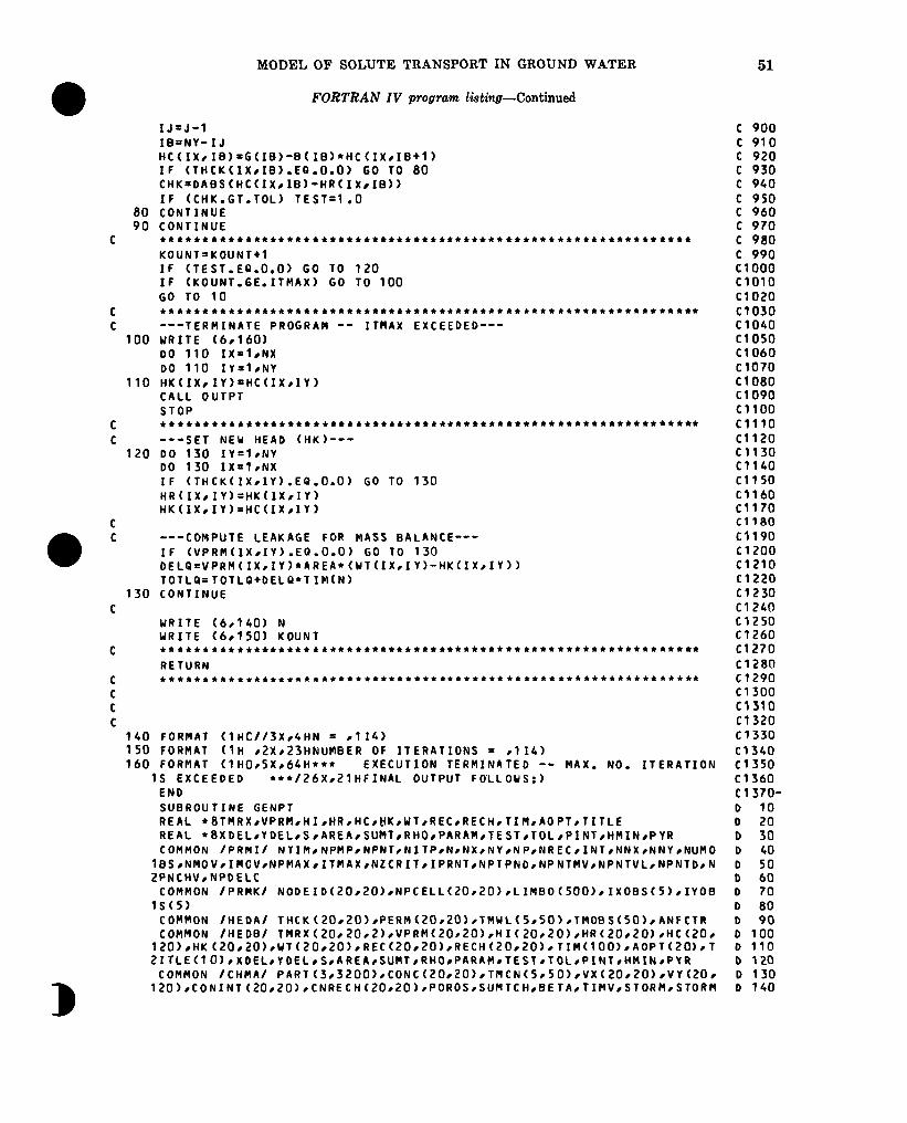
C
C C
C C
C C
MODEL OF SOLUTE TRANSPORT IN GROUND WATER
FORTRAN IV program listing-Continued
IJ=J-1 IB=NY-IJ HC~IX~IB~=G~IB~-B~I~~*HC~IXIIB*1~ IF (THCK(IX~IB).EQ.O.O) GO TO 80 CHK=DABS(HC(IXIIB)-HR(IX#IB)) IF tcttK.GT.To~) TEST=1 .O
80 CONTINUE 90 CONTINUE
t***t***~************ttt**tt+**~~**~~**~~~~*~*~~*~~~***~~**~~*~~*~~~ KOUNT=KOUNT+l IF (TEST.EQ.O.0) GO TO 120 IF (KOUNT.GE.ITflAX) GO TO 100 GO TO 10 *t+**Zt+*t**++**C+t**C+**C1++*t**tl*++t*~~~*.~~~~~~~~..~~~~~~~~* ---TERMINATE PROGRAN -- ITRAX EXCEEDED---
100 WRITE (6,160) DO 110 IX=lrNX DO 110 IY=lrNY
110 HK(IXIIY)‘HC(IXIIY) CALL OUTPT STOP tttt********t**tt***~~~~~~~*****t*~*~*~~*~~**~~***~~*~*~~* ---SET NEW HEAD (HK)---
120 DO 130 IY=lrNY DO 130 IX=lrNX IF (THCK(IX.IY).EP.O.O) GO TO 130 HR(IXIIY)=HK(IXIIY) HK(IX,IY)=HC(IXIIY)
---COMPUTE LEAKAGE FOR MASS BALANCE--- IF (VPRM(IX,IY).EQ.O.O) GO TO 130 DELP=VPRM(IX,IY)*AREAIo-HK(IX,IY~-HK(IX,IY)) TOTLP=TOTLQ+DELQ*T IM(N)
130 CONTINUE
140 FORMAT tlHC//3X,bHN = rl 14) 150 FORMAT (1H rZX,23HNUMBER OF ITERATIONS = ,114) 160 FORMAT (1 H015X#64H*+* EXECUTION TERMINATED -- MAX. NO. ITERATION
1S EXCEEDED l ++/26X,2lHFINAL OUTPUT FO’LLOWS:) END SUBROUTINE GENPT REAL *~TMRX,VPRM,HI,HR~HC~~K~WTIREC,RECHITIMIAOPT~TITLE REAL *~XDELIYDELISIAREAISUMT~RHO~PARA~~TESTITOL~PXNT~HMIN~PYR COMMON /PRMI/ NTIMINPMPINPNTINITPININXINYINPINRECIINTINNX~NNY~NUMO
lBSINfl0vII~0vl~p~A~I~TNA~~N2CR~T~IpRNTI~~Tp~~,~p~T~~,~~~T~~,NpNT~,N ZPNCHVINPDELC
COMMON /PRMK/ NODEID~20,20~.NPCELL~20.20~,LIMBO~500~rIXOBS~5~,IYOB lS(5)
COMMON /HEDA/ THCK(~O.~~)~PERM(~~IZO)~TMWL~~,~~~.TMOBS~~O~,ANFCTR COMMON /HEDB/ TMRX~20~20,2~rVPRM~20~20~~H1~20~20~rHA(Z0~20~~HC~20~
120~rHK~2O,20~rWT~2O,20~.REC~20~20~,RECH~20.2O~.TIM~lOO~.AOPT~20~,T ~ITLE~~~~~XDEL~YDEL~S,AREA~SUMT~RHO~PARAN~TEST~TOLNPINT~HMIN~PYR
COMMON /CHMA/ PART(3r3200),CONC(2OIZO)rTMCN(5r50)*VX(20~20)~VY(20~
51
c 900 c 910 C 920 c 930 c 940 c 950 C 960 c 970 C 980 c 990 c1000 Cl010 Cl020 Cl030 Cl040 Cl050 Cl 060 Cl070 Cl080 Cl090 Cl100 Cl110 Cl120 Cl130 Cl140 Cl150 Cl160 Cl170 Cl180 Cl190 Cl200 Cl210 Cl 220 Cl 230 Cl 240 Cl250 Cl260 Cl270 Cl280 Cl290 Cl 300 Cl310 Cl 320 Cl 330 Cl340 Cl350 Cl360 c 1370- D 10 D 20 D 30 D 40 D 50 D 60 D 70 D 80 D 90 D 100 D 110 D 120 D 130
12O~,CONINT~2O.2O~rCNRECH~2O~2O~~POROS~SURTCH~BETA~TIRV~STORR~STORR D 140

52 TECHNIQUES OF WATER-RESOURCES INVESTIGATIONS
FORTRAN IV program listing-Continued
ZIrCHSIN~CMSOUT~fLWINIFLMOTISUHIO~CELDIS~DLlRAl~CSlORM DIMENSION RP(8)r RN(8)r IPT(8) *****************t*****t**t****t************************************ Fls0.30 f2=1.0/3.0 If (NPTPND.EQ.4) flrO.25 If (NPTPND.EQ.9) f 1=1.0/3.0 If (NPTPND.EQ.8) F2~0.25 NCHK=NPTPND If (NPTPND.EQ.S.OR.NPTPND.EQ.9) NCHK=NPTPND-1 IF (TEST.GT.98.) GO TO 10 **+*******************w************~*************************** ---INITIALIZE VALUES--- STORM-0.0 CMSIN=O.O CMSOUT-0.0 FLIIIN-0.0 f LMOTrO.0 suR10~0.0 **********+****************************************************
10 DO 20 ID=),3 DO 20 IN=lrNPMAX
20 PART(IDIIN)=O.O DO 30 IA=lr8 RP(1A)rO.O RN(1A)rO.O
30 IPT(IA)=O ---SET UP LIMO0 ARRAY--- DO 40 IN=lrSOO
40 LIH8O(IN)~O.O IND=l DO 50 IL=lr50012 LlMEO(IL)=IND
50 IND=IND+l *******+****+**+*********************************************** ---INSERT PARTICLES--- DO 410 IX=leNX DO 610 IY=leNY IF (THCK(IX,IY).EQ.O.O) GO TO 410 KR=O TESTZ=O.O METH=l NPCELL(Ix,IY)=O Cl=CONC(IX,IY) If (Cl.LE.l.OE-03) TEsT211.0 IF (VPRM(IX,IY).GT.O.O9) TEST2nl.O IF (REC(IXIIY).NE.O.O) TESTtrl.0 If ~THCK~IX+1.IY+l~.EQ.O.O.OR.THCK~IX*lrIY-l~.EQ.O.O.OR.THCK~IX-l,
lIY+l).EQ.O.O.OR.THCK(IX-l#IY-l).EQ.O.O) TEST2t1.0 IF ~~THCK~IX~IY+~~.EQ.O.O.OR~THCK~IX,IY-~~.EQ.O.O.OR.THCK~IX+~.IY~
1.EQ.O.O.OR.THCK~IX-l,IY~.EQ.O.O~.AND.NPlPND.GT.S~ TESTZ=l.O CNODE=Cl*(l.O-F1) If (TEST.LT.98.0.0R.TEST2.GT.O.O) GO TO 70 SUMC=CONC~IX+?rIY~tCONC~IX-1~~Y~tCONC~IX~IYtl~tCONC~IX~IY-l~ IF (NCHK.EQ.4) GO TO 60 SU~C~SUMC+CONC~IX+lrIY+l~tCONC~~X+l.IY-1~tCONC~IX-l,IYtl~tCONC~IX-
ll,IY-1) 60 AVC=SUMC/NCHK
If (AVC.GT.Cl) PlETH=2 C C ---PUT L PARTICLES ON CELL DIAGONALS---
70 DO 140 IT=1#2
- D 150 D 160 D 170 D 180 D 190 D 200 D 210 D 220 D 230 D 240 D 250 D 260 D 270 D 280 D 290 D 300 D 310 D 320 D 330 D 340 D 350 D 360 D 370 D 380 D 390 D 400 D 410 D 420 D 430 D 440 D 430 D 460 D 470 D 480 D 490 D 500 D 310 D 520 D 530 D 540 D 330 D 560 D 570 D 580 D 590 D 600 D 610 D 620 D 630 D 640 D 650 D 660 D 670 D 680 D 690 D 700 D 710 D 720 D 730 D 740 D 750 D 760
c

MODEL OF SOLUTE TRANSPORT IN GROUND WATER 53
FORTRAN IV program listing-Continued
EVET=(-1 .o)**IT DO 140 IS=lrZ EVES=(-l.O)**IS PART(1 rIND)=IX+Fl+EVET PART(2tIND)=IY+Fl*EVES PART(ZIIND) =-PART (2,IND) PARTOrIND)=Cl IF (TEST.LT.98.0.0R.TESTZ.CT.O.O.O) GO TO 130 IXD=IX+EVET IYD=IY+EVES KR=KR+l IPT(KR)=IND IF (METH.EP.2) GO TO 80 PART(3rIND)=CNODE+CONC~IXD,IYD)*Fl GO TO 90
80 PART~3rIND~=2.O*Cl*COMC~IXD~IYD~/~C1~CONC~IXD.IYD~~ 90 IF (Cl-CONC(IXDIIYD)) 10011101120
100 RP(KR)=CONC(IXD,IYD)-PART(3rINb) RNCKR)=Cl-PART(3rIND) GO TO 130
110 RP(KR) -0.0 RN(KRIrO.0 GO TO 130
120 RP(KR)=Cl-PARTCSIIND) RN(KR)=CONC(IXDeIYD)-PART(3,IND)
130 IND=IND+l 140 CONTINUE
C IF <NPTPND.EQ.~.OR.NPTPND.EQ.9) GO TO 150 GO TO 160
C ---PUT ONE PARTICLE AT CENTER OF CELL--- 150 PART(lrIND)=-IX
PART(~IIND)=-IY PART(3rIND)‘Cl IND=IND+l
C ---PLACE NORTH@ S~IJTHI EASTI AND UEST PARTICLES--- 160 IF (NPTPND.LT.8) GO TO 290
CNODE=Cl*(l.O-F2) DO 280 IT=lrZ EVET=(-l.O)*+IT PART(1 rIND)=IX+FZ*EVET PART(Z,IND)=-II PART(3rIND)rCl IF (TEST.LT.98.0.0R.TESTZ.GT.O.O.O) GO TO 220 IXD=IXtEVET KR=KRtl IPT(KR)=IND IF (METH.E0.2) GO TO 170 PART(3rIND)=CNODEtCONC(IXDIIV)+fZ GO TO 180
170 PART~3rIND~=2.O*Cl~CONC~IXDIIV)/(C1tCONC~IXD,IY~~ 180 IF (Cl-CONCCIXbrIY)) 19012001210 190 RP(KR)=CONC(IXDIIY)-PART(3rIND)
RN(KR)=Cl-PART(3,IND) GO TO 220
200 RP(KRIrO.0 RN(KR)=O.O GO TO 220
210 RP(KR)=Cl-PARTC3,IND) RN<KRl=CONC(IXDrIY)-PART(3rIND)
220 IND=INDtl PART<1 rIND)=IX
D 770 D 780 D 790 D 800 D 810 D 820 D 830 D 840 D 850 D 860 D 870 D 880 0 890 D 900 D 910 D 920 D 930 0 940 0 950 D 960 0 970 D 980 D 990 DlOOO 01010 DlO20 01030 D1040 D1050 D1060 D1070 01080 01090 Dl100 D1110 D1120 01130 01140 01150 01160 01170 01180 Dl190 01200 D1210 D1220 01230 D1240 01250 D1260 01270 D1280 01290 01300 01310 01320 01330 D1340 01350 Dl360 01370 01380

54 TECHNIQUES OF WATER-RESOURCES INVESTIGATIONS
FORTRAN IV program &ding-Continued
PARTCZ,IND)=IYtF2*EVET PARTCZIIND) =-PARTCZIIND) PARTC3,IND)=C1 IF CTEST.LT.98.0.0R.TESTZ.GT.O.O) GO TO 280 IYD=IYtEVET KR=KRtl IPTCKR)=IND IF CMETH.EQ.2) GO TO 230 PARTC3/IND)=CNODEtCONC(IX,IYD~*F2 GO TO 240
230 PART~3rIND~=2.O*Cl*CONC~IX~IYD~/~CltCONC~IX,IYD~~ 240 IF (Cl-CONC(IX,IYD)) 250#260/270 250 RPCKR)=CONCCIX,IYD)-PART(3rlND)
RNCKR)=Cl-PARTC3rIND) GO TO 280
260 RPCKR) =O.O RNCKR) 10.0 GO TO 280
270 RPCKR) =Cl-PARTC3rIND) RNCKR)=CONCCIXIIYD)-PART(3rIND)
280 IND=INDtl C
290 IF CTEST.LT.98.O.OR.TESTZ.GT.O.O) GO TO 410 SUMPT’O.0
C ---COMPUTE CONC. GRADIENT WITHIN CELL--- DO 300 KPT=lrNCHK IK=IPT (KPT)
300 SUMPT=PARTC3rIK)tSUMPT CBAR=SUMPT/NCHK
C ---CHECK MASS BALANCE WITHIN CELL AND ADJUST PT. CONCS.--- SUHPTnO.0 IF CCBAR-Cl) 310r410r330
310 CRCf=l ,O-<CBAR/Cl) IF CMETH.EQ.1) CRCT=CBAR/Cl DO 320 KPT=lrNCHK IK=IPT <KPT) PARTO,IK)=PARTC3,IK)tRPCKPT)*CRCT
320 SUMPT=SUMPTtPARTC3rIK) CBARN=SUMPT/NCHK GO TO 350
330 CRCT=l.O-CCl/CBAR) IF CMETH.EQ.1) CRCT=Cl/CBAR DO 340 KPT=lrNCHK IK=IPT CKPT) PARTC3rIK)=PARTC3,IK)tRNCKPT)*CRCT
340 SUMPT=SUMPTtPARTC3rIK) CBARN=SUMPT/NCHK
350 IF CCBARN.EQ.Cl) GO TO 410 C ---CORRECT FOR OVERCOMPENSATION---
CRCT=Cl/CBARN DO 380 KPT=lrNCHK IK=IPT CKPT) PARTC3rIK)=PART<3rIK)*CRCT
C ---CHECK CONSTRAINTS--- IF CPARTC3rIK)-Cl) 360r380r370
360 CLIM=Cl-RPCKPT)tRNCKPT) I,F CPARTC3rIK).LT,CLIM) GO TO 390 GO TO 380
370 CLIM=C1tRP(KPT)-RN(KPT) IF CPARTC3rIK).GT.CLIH) GO TO 390
380 CONTINUE GO TO 410
D1390 Dl400 Dl410 D1420 D1430 D1440 D1450 01460 D1470 D1480 D1490 01500 01510 01520 01530 Dl540 Dl550 Dl560 Dl570 D1580 D1590 Dl600 D1610 D1620 D1630 D1640 D1650 01660 D1670 01680 01690 01700 01710 D1720 01730 01740 D1750 Dl760 D1770 01780 D1790 D1800 01810 D1820 D1830 D1840 Dl850 D1860 01870 D1880 Dl890 Dl900 01910 D1920 D1930 D1940 D1950 01960 D1970 01980 D1990 02000
c

MODEL OF’ SOLUTE TRANSPORT IN GROUND WATER 55
FORTRAN IV program listing-Continued
390 TESTZ-1.0 DO 400 KPT=lrNCHK IK=IPTCKPT)
400 PARTC3#IK)=Cl 410 CONTINUE
NP=INO IF CINT.EP.0) CALL CHMOT
C **t*t*t******ttt**tt**t*t*************t****~~~~*~~~~~~~~~~.~~~~~ RETURN
C t+ttt****+**tt****tt****22*t*tt*t*t***t*~*~~*~*~~~~~*~*~*~**~~~* END SUBROUTINE VELO DOUBLE PRECISION DMIN~~DEXPIDLOGIDABS REAL +8TMRX~VPRM~HI~HR~HC,HK,WT,RECIRECH,TIM,AOPT~TITLE REAL *~XDELIYDELIS,AREA,SUMT,RHO,PARAM,TEST,TOL~PINT,HMIN,PYR REAL +~RATEISLEAKIDIV COMMON /PRMI/ NTIMINPMPINPNTINITPIN,NXINYINPINRECIINTINNX~NNY~NUMO
1BS8NM0v~IMCv~NpMAX~ITMAX0N2C~IT,IpR~TI~pTp~~,~p~T~~,~~~~~~,Np~T~,~ ZPNCHV,NPDELC
COMMON /PRMK/ NODEID~2O,2O~rNPCELL~2O,2O~,LIMBO~5OO~,IXOBS~5~,IYOB IS(S)
COMMON /HEDA/ THCK~20~20~rPERM~20,20~~TMWL~5~50~~TM0BS~50~~ANFCTR COMMON /HEDB/ TMRX~20~20~2~rVPRM~20IZO),H1~20~20~~HR~20~20~~HC~20,
~~~~~~~~~~~~~~~~~~~~~~~~~~~~~~~~~~~~~~~~~~~~~~~~~~~~~~~~~~~~~~~~~~~ 2ITLE~lO~rXDEL~YREL~S~AREA,SUMT,RHO,PARAM,TEST,TOL~PINT,HMIN,PYR
COMMON /XINV/ DXINVIDYINVIARINVIPORINV COMMON /CHMA/ PART~3r3200~,C0NC~20,20~,TMCN~5,50~,VX~20,20~,VY~20,
12O~rCONINT~2O,2O~rCNRECH~2O,2O~rPOROS,SUMTCH,BETA,TIMV,STORM,STORM 2I~CMSIN~CMSOUT~FLMIN,FLMOT,SUMIOICELDIS~DLTRAT~CSTORM
COMMON /CHRC/ SUMC(20~20)rVXBDYC20,20~.VYBDYC20,20) COMMON /DIFUS/ DISPC20120e4)
C *****t+t******+*+t~**t****ttt*****ttt******************************~~~ C ---COMPUTE VELOCITIES AND STORE---
VMAX=l .OE-10 VMAY=l .OE-10 VMXBD=l .OE-10 VMYBD=l .oE-10 TMV=TIMCN) LIM=O
C DO 20 IX=lrNX DO 20 IY=lrNY DO 10 IZ=lr4
10 DISPCIXIIYIIZ)=O.O c
IF CTHCKCIXIIYT.EQ.O.O) GO TO 20 RATE=RECCIXIIYT/AREA SLEAK=CHKCIX.IY)-WTCIX.IY~~*VPRMCIX~IY) DIV=RATE+SLEAK+RECHCIXIIY)
C C ---VELOCITIES AT NODES--- C ---X-DIRECTION---
GRDX=CHKCIX-l,IY)-HK(IX+lrIY))*DX1NV*0.50 IF CTHCKCIX-lrIY1.EQ.O.O) GRDX=(HK(IXIIY)-HKCIX+lrIY))*DXINV IF CTHCKCIX+l~IY).EQ.O.O) GRDX’CHK(IX-lrIY)-HKo)*DXINV IF CTHCKCIX-lrIY).EQ.O.O.AND.THCKCIX+l,IY).EQ.O.O~ GRDX=O.O VXCIX~IY)=PERMCIX~IY)*GRDX*PORINV ABVX=ABS(VX(IXn IY 1) IF (ABVX.GT.VMAX) VMAX=ABVX
C ---Y-DIRECTION---
B
GRDY=CHKCIX~IY-1)-HK(IXIIY*1))*DYINV+O.SO IF CTHCKCIXIIY-l).EQ.O.O) GRDY=CHKCIXeIY)-HKCIXIIY+1))*DYINV
D2010 D2020 02030 02040 02050 02060 02070 02080 D2090 D2100 D2110- E 10 E 20 E 30 E 40 E 50 E 60 E E 2 E 90 E 100 E 110 E 120 E 130 E 140 E 150 E 160 E 170 E 180 E 190 E 200 E 210 E 220 E 230 E 240 E 250 E 260 E 270 E 280 E 290 E 300 E 310 E 320 E 330 E 340 E 350 E 360 E 370 E 380 E 390 E 400 E 410 E 420 E 430 E 440 E 450 E 460 E 470 E 480 E 490 E 500 E 510

56 TECHNIQUES OF WATER-RESOURCES INVESTIGATIONS
FORTRAN IV program listing--Continued
IF (THCK(IX,IY+l).EQ.O.O) GRDY=(HK(IX~IY-l)-HK(IXIIY))*DYINV IF (THCK(IX,IY-l).EQ.O.O.AND.THCK(IXllr*1).EQ.O.O~ GRDY-0.0 VY(IX,IY)=PERM(IX,lY)*GUDY*PORINV*ANFCTR ABVY=AES(VY(IXIIY)) IF (ABVY.GT.VMAY) VMAY=ABVY
C C ---VELOCITIES AT CELL BOUNDARIES---
GRDX=(HK(IXIIY)-HK(IX+l<IY))*DXINV PERMX=2.O*PERM~IX,IY~*PERM~IX+lrIY~/~PERM~IX~IY~+PERN~IX+l~IY~~ VXBDY(IX~IY)=PERMX*GRDX*PORINV GRDY=(HK(IXIIY)-HK(IX,IY+l))*DYINV PERMY=2.O*PERM~IX~IY~*PERM~IX,IY+l~~~PERM~IX~IY~+PERM~IX~IY+l~~ VYBDY(IX~IY)=PERMY*GRDY*PORINV*ANFCTR ABVX=ABS(VXBDY(IXIIY)) ABVY=ABS(VYBDY(IXIIY)) IF (ABVX.GT.VMXBD) VMXBD=ABVX IF (ABVY.GT.VMYBD) VRYBD'ABVY
c
IF (DIV.GE.O.0) GO TO 20 TDIV=(POROS*THCK(IX~IV))IDABS(DIV) IF (TDIV.LT.TMV) TMV=TDIV
20 CONTINUE C ****************t********************************************** C ---PRINT VELOCITIES---
IF (NPNTVL.EQ.0) GO TO 80 IF (NPNTVL.EQ.2) GO TO 30 IF (NPNTVL.EQ.l.AND.N.EQ.1) GO TO 30 GO TO 80
30 WRITE (6r320) WRITE (6r330) DO 40 IY=lrNY
40 WRITE (6r350) (VX(IXIIY)~IX=~~NX) WRITE (6r340) DO 50 IY=lrNY
50 WRITE (6r350) (VXBDY~IXIIY)~IX=~,NX) WRITE (6r360) WRITE (6r330) DO 60 IY=lrNY
60 WRITE (6r350) (VY(IXrIY)rIX=lrNX) WRITE (6r340) DO 70 IY’lrNY
70 WRITE (6r350) (VYBDY(IX,IY)~IX+~~NX~ C ---PUNCH VELOCITIES---
80 IF (NPNCHV.EQ.0) GO TO 110 IF (NPNCHV.EQ.2) GO TO 90 If (NPNCHV.EQ.1.AND.N.EQ.l) GO TO 90 GO TO 110
90 WRITE (7rS101 NXINYIXDEL~YDELIVMAXIVMAY DO 100 IY'lrNY WRITE (7r520) (VX(IX~IY)rIX=lrNX)
loo WRITE (7.520) (VY(IX.IY)rIX=lrNX) C ****************************************************************
C ---COf4PUTE NEXT TINE STEP--- 110 WRITE (6r390)
WRITE (6,400) VHAXIVHAY WRITE (6r410) VMXBDeVMYBD TDELX-CELDIS*XDEL/VMAX TDELY=CELDIS*YDEL/VMAY TDELXB=CELDIS*XDEL/VMXBD TDELYB=CELDIS*YDEL/VHYBD TIMV=ARINl(TDELX,TDELYITDELXBeTDELYB) WRITE (6.310) TMVeTIMV
E 520 E 530 E 540 E 550 E 560 E 570 E 580 E 590 E 600 E 610 E 620 E 630 E 640 E 650 E 660 E 670 E 680 E 690 E 700 E 710 E 720 E 730 E 740 E 750 E 760 E 770 E 780 E 790 E 800 E 810 E 820 E 830 E 840 E 850 E 860 E 870 E 880 E 890 E 900 E 910 E 920 E 930 E 940 E 950 E 960 E 970 E 980 E 990 El000 El010 El020 El030 El040 El050 El060 El070 El080 El090 El100 El110 El120 El130
c
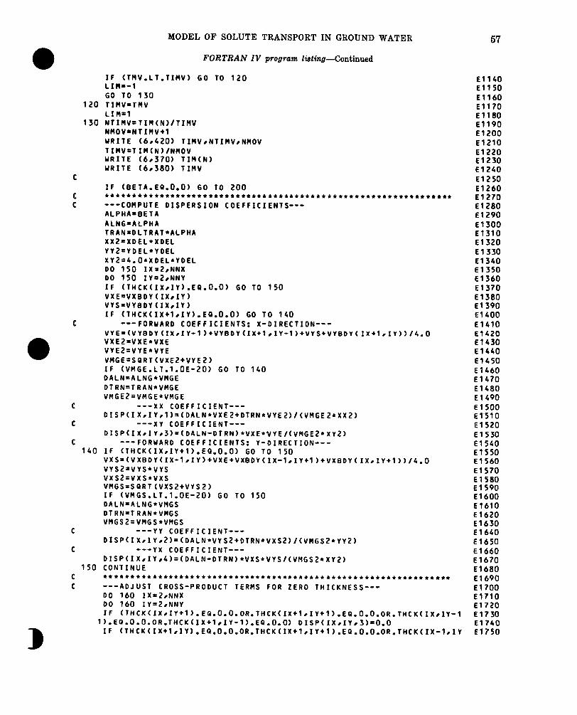
MODEL OF SOLUTE TRANSPORT IN GROUND WATER
FORTRAN IV program listing-Continued
IF CTHV.LT.TIHV) GO TO 120 LIW-1 GO TO 130
120 TIHV=TRV LIMMl
130 NTIMV=TIMCN)/TIMV NMOVfNTIHV+l WRITE (6r420) TIMVINTIMVINMOV TINV=TIMCN)/NMOV WRITE (6r370) TIM(N) WRITE (6r380) TIMV
C IF (BETA.EO.O.0) GO TO 200
C **************************************************************** C ---COtlPUTE DISPERSION COEFFICIENTS---
ALPHAsBETA ALNG'ALPHA TRAN=DLTRAT*ALPHA XXZ=XDEL*XDEL YY2'YDEL*YDEL XY2=4.O*XDEL*YDEL DO 150 IX=ZtNNX DO 150 IYM2eNNY IF CTHCKCIXIIY).EQ.O.O) GO TO 150 VXE=VXBDYCIXIIY) VYS=VYBDYCIX,IY) IF CTHCKCIX+l~IY).EQ.O.O) GO TO 140
C ---FORWARD COEFFICIENTS: X-DIRECTION--- VYE=~VYBDY~IX.IY-l~+VY~DY~IX+~.IY-l~+VYS+VYBDY~IX+l,IY~~/4.O VXEZ=VXE*VXE VYEZ=VYE*VYE VMGE=SQRTCVXEZ+VYE2) IF CVMGE.LT.l.OE-20) GO TO 140 DALN=ALNG*VHGE DTRN=TRAN*VMGE VMGEZ=VMGE*VMGE
C ---XX COEFFICIENT--- DISPCIX,IY,l)=CDALN*VXEZ*6fRN+VYEZ)/(VnGE2*XX2~
C ---XY COEFFICIENT--- DISP(IXIIYI~)=(DALN-DTRN)*VXE*VYEI(VnCEZ*XY2)
C ---FORWARD COEFFICIENTS: Y-DIRECTION--- 140 IF CTHCKCIX~IY+l).EQ.O.O) GO TO 150
VXS=~VXBDY~IX-lrIY~+VXEtVXBDY~IX-l.IY+1~tVXBDY~IX.IYtl~~/4.O VYS2fVYS*VYS vxs2=vxs*vxs VMGS=SQRTCVXSZ*VYSZ) IF CVMGS.LT.l.OE-20) GO TO 150 DALN=ALNG*VMGS DTRN=TRAN*VMGS VMGS2=VMGS*VMGS
C ---YY COEFFICIENT--- DISPCIX~IY~2)=CDALN*VYS2+OTRN+VXSZ)/(VMCS2*YY2)
C ---YX COEFFICIENT--- DISPCIXIIYI~)=CDALN-DTRN)*VXS*VYS/(VMCSZ*XY2)
150 CONTINUE C *************t************************************************** C ---ADJUST CROSS-PRODUCT TERMS FOR ZERO THICKNESS---
DO 160 IX=ZINNX DO 160 IY=ZeNNY
57
El140 El150 El160 El170 El180 El190 El200 El210 El220 El230 El240 El250 El260 El270 El280 El290 El300 El310 El320 El330 El340 El350 El360 El370 El380 El390 El400 El410 El420 El430 El440 El450 El460 El470 El480 El490 El500 El'310 ElS20 El530 El540 El550 El560 El570 ElS80 El590 El600 El610 El620 El630 El640 El650 El660 El670 El680 El690 El700 El710 El720
IF ~THCK~IX~IY+1~.EQ.O.O.OR.THCK~IX~1~IY~1~.EQ.O.O.OR.THCK~IX~IY-l El730 l).EQ.O.O.OR.THCK(IX+l.IY-l).EQ.O.O) DISP(IXeIYr3)=0.0 El 740
IF ~THCK~IX*lrIY~.EQ.O.O.OR.THCK~IX*lrIY*1~.EQ.O.O.OR.THCK~IX-1,IY El750

68 TECHNIQUES OF WATER-RESOURCES INVESTIGATIONS
FORTRAN IV program listing-Continued
l).EQ.O.O.OR.THCKCIX-l#IY+l).EQ.O.O) DISPCIX,IYI~)=O.O 160 CONTINUE
C t2**t****ttt****t***~~~~~~~*~*~*~~~*****~~*~~~~~~~~~*~~*~*4*~~*~ C ---CHECK FOR STABILITY OF EXPLICIT RETHOD---
TIMDIS'O.0 DO 170 IX=ZINNX DO 170 IY=ZINNY TDCO=DISP<IX,IY,?)+DISP(IXIIYlt)
170 IF CTDCO.GT.TIMDIS) TIMDIS=TDCO TIHDC=O.3/TIMDIS URITE (6~440) TIMDC NTIMD=TIMCN)/TIMDC NDISP=NTIHD+l IF CNDISP.LE.NMOV) GO TO 180 NMOV=NDISP TIMV~TIMCN)/NMOV LIM=O
180 WRITE (6r430) TIMVINTIMDINMOV C t+**,+*ttttl***t~****t**+*t*tt**ttt*t*+t~*~~****~*~*~~~**~~~**** C ---ADJUST DISP. EQUATION COEFFICIENTS FOR SATURATED THICKNESS---
DO 190 IX-28NNX 00 190 IY=2rNNY BAVX=O.3*CTHCKCIX~IY)+THCK(IX+lrIY)) l3AVY=O.S*CTHCKCIX~IY)+THEK(IX~IY+l)) DISPCIX~IY~1)=DISPCIXIIVI1)*BAVX DISPCIXIIY,~)=DISPCIXIIYIZ)+BAVY DISPCIX~IY~3)=DISPCIXIIrr3)*BAVX
190 DISPCIXIIY~~)=DISPCIXIIYI~)+~AVY C *t**************tt***************************,************~*****
200 IF CLIM) 210122Ot230 210 WRITE (6r530)
GO TO 240 220 URITE (6.540)
GO TO 240 230 WRITE (6rSSO)
C **t*t~t***+~t~t+t**~t+t**~*~~~*~~~~~***~*******~*************~~*~** C ---PRINT DISPERSION EQUATION COEFFICIENTS---
240 IF CNPNTD.EQ.0) GO TO 300 IF CNPNTD.EQ.2) GO TO 250 IF CNPNTD.EQ.l.AND.N.EQ.1) GO TO 250 GO TO 300
250 WRITE (6,450) WRITE (6.460) DO 260 IY=lrNY
260 WRITE (6.500) CDISPCIXIIY,~),IX=~~NX) WRITE C6#470) DO 270 IY=lrNY
270 WRITE (6rSCO) CDISPCIXIIYI~)~IX=~~NX) WRITE (6.480) DO 280 IY=lrNY
280 WRITE (6rSOO) CDISPCIXIIY~~)~IX=~~NX) WRITE (6.490) DO 290 IY=lrNY
290 WRITE (60500) CDISPCIXIIYI~)~IX=~~NX) C ***+***t+***t*******~~~~~~~*.~~~~~~~~~~~~~~~.~~~~*~~~*4~~4~~~~~*
300 RETURN C +tt*ttt*t*t****+***t+****tt2************.~**~******~*4*4~~~*~~~~~~~*~*
c’ C
El760 El770 El780 El790 El800 El810 El820 El830 El840 El850 El860 El870 El880 El890 El900 El910 El 920 El930 El940 El950 El960 El970 El 980 El990 E2000 E2010 E2020 E2030 E2040 E20S0 E2060 E2070 E2080 E2090 E2100 E2t10 E2120 E2130 E2140 E21 SO E2160 E2170 E2180 E2190 E2200 E2.210 E2220 E2230 E2240 E2250 E2260 E2270 E2280 E2290 E2300 E2310 E2320 E2330 E2340 E2350
310 FORMAT ClW r19H TMV (MAX. INJ.) = rG12.5/20H TImv CCELDIS) = l G E2360 112.5) E2370
c

MODEL OF SOLUTE TRANSPORT IN GROUND WATER
FORTRAN IV program listing-Continued
320 FORMAT C1HlrlZHX VELOCITIES) 330 FORMAT ClH ,25X,8HAT NODES/) 340 FORMAT (lH0125X~l3HON BOUN’DARIES/) 350 FORMAT ClH r10G12.3) 360 FORMAT ClHlrl2HY VELOCITIES) 370 FORMAT C3H rllHTIM CN) = rlG12.5) 380 FORMAT (3H rllHTIMEVEL0 = rlG12.5) 390 FORMAT C~H~~~~XI~~HSTABILITY CRITERIA --- H.O.C.//) 400 FORMAT ClH008H VMAX = rlPE9.2,5X17HVblAY = rlPE9.2) 410 FORMAT ClH r8H VMXBD= ,~PEP.Z,SXI~HVMYBD= rlPE9.2) 420 FORMAT ClH0,8H TIMV = rlPE9.215X~8HNTIMV = ,15,5X,7HNMOV = ,15/j 430 FORMAT Cl H0e8H TIMV = rlPE9.2eSX,8HNTIMD = ,IS,SX,7HNMOV = ,151 440 FORMAT C3H rllHTIMEDISP = rlE12.5) 450 FORHAT ClHlr32HDISPERSION EQUATION COEFFICIENTS,~~XI~~H=CD-IJ)*CB)
l/CGRID FACTOR)) 460 FORMAT ClH r35X114HXX COEFFICIENT/) 470 FORMAT ClH r35X114HYY COEFFICIENT/) 480 FORMAT ClH r35X114HXY COEFFICIENT/) 490 FORMAT ClH r35X114HYX COEFFICIENT/) 500 FORMAT ClH rlP10E8.1) 510 FORMAT (214r2FlO.lr2F10.7) 520 FORMAT (8F10.7) 530 FORMAT C~HO,~OXI~~HTHE LIMITING STABILITY CRITERION IS CELDIS) 540 FORMAT ClHC,lOX,40HTHE LIMITING STABILITY CRITERION IS BETA) 550 FORMAT (lHO.lOX,58HTHE LIMITING STABILITY CRITERION IS MAXIMUM INJ
1ECTION RATE) END SUBROUTINE MOVE REAL *~TMRXIVPRMIHIIHRIHCIHKIWTIRECIREC,RECH~TIM,AOPT.TI~LE REAL *~XDELIYDELISIAREAISUMTIRHOIPARAMITESTITOL~PINT~HMIN,PYR COMMON /PRMI/ NTIM~NPMPINPNTINITPIN~NX~NY~NP~NREC~INT~NNX~NNY~NUMO
lBSINM0~IIM0vlNpMAxIITMA~~N2CRIT~IpR~TlNpTpN0~N~NTMv~N~~~~~8~~~~~,~ 2PNCHV,NPDELC
COMMON /PRMK/ NODEID~2O,2O~rNPCELL~2O,2O~,LIMBO~5OO~.IXOES~S~,IYOB 1SCS)
COMMON /HEDA/ THCK(~~I~~),PERM(~O,~O~~TMWL~S~~~~~TMOBS~~~~,ANFCTR COMMON /HEDB/ TMRX(~~I~~I~),VPRM(~~,~~)~HI(~~),HR(Z~,~~).HC(~~,
12O~,HK~2O,20~rWT~20IZO)rRECorREC~20~2O~~RECH~20~20~,TIN~l00~,AOPT~20~,T ~ITLE(~~)~XDELIYDELISIAREAISUMTIRHO,PARAM~TEST~TOL~PINT~HMIN,PYR
COMMON /xINV/ DXINV~DYINVIARINVIPORINV COMMON /CHMA/ PART(3r3200lrCONC(20IZO)rTMtNorVX(Z0,20~~VY~20,
l2O~,CONINT~20,2O~rCNRECH~2O,2O~rPOROS,SUMTCH,BETA,TIMV,STORM,STORM ~I~CHSINICMSOUTIFLMIN,FLMOTISUMIOICELDIS~DLTRAT~CSTORN
COMMON /CHMC/ SUMCC~~I~~).VXBDYC~O~~~),VYBDYC~~.~~) DIMENSION XNEW(4)r YNEWC4)r DIST(4)
C ***+~t****t*t*****+t***+t**t**+tt*+**+*t~~.~~~~~~~~~~...~~~.~~~ WRITE (6r680) NMOV SUMTCH=SUMT-TIM(N) Flt0.249 IF CNPTPND.EQ.5) FlrO.299 IF CNPTPND.EQ.9) F1=0,333 CONSTl =TIMV*DXINV CONSTZ=TIMV*DYINV
C ---MOVE PARTICLES ‘NMOV’ TIMES--- DO 650 IMOV=lrNMOV
10 NPTM=NP C ---MOVE EACH PARTICLE---
DO 590 IN=lrNP IF CPARTClrIN).EQ.O.O) GO TO 590 KFLAG=O
C ******tC*****t*+*t**t*+t*+tt+******t****~~*~~~**~~~*~~~*~~*~~~~ C ---COMPUTE OLD LOCATION---
E2380 E2390 E2400 E2410 E2420 E2430 E2440 E2450 E2460 E2470 E2480 E2490 E2500 E2510 E2520 E2530 E2540 E25SO E2560 E2570 E2S80 E2590 E2600 E2610 E2620 E2630 E2640- F 10 F 20 F 30 F 40 F 50 F 60 F 70 F 80 F 90 F 100 F 110 F 120 F 130 F 140 F 150 F 160 F 170 F 180 F 190 F 200 F 210 F 220 F 230 F 240 F 250 F 260 F 270 F 280 F 290 F 300 F 310 F 320 F 330 F 340 F 350
59

60 TECHNIQUES OF WATER-RESOURCES INVESTIGATIONS
FORTRAN IV program listing--Continued
JFLAG=l F 360 IF cPARTcl,IN).GT.O.OI GO TO 20 F 370 JFLAG=-1 F 380 PAATcl,IN) =-PARTclrIN) F 390
20 XOLD=PARTclrIN) F 400 IX=XOLD+O.S F 410 IFLAG' F 420 IF cPARTc2,INI.GE.O.O) GO To 30 F 430 IFLAG=-l F 440 PARTcZ,IN)=-PARTCZIIN) F 450
30 YOLD'PARTC~IIN) F 460 IY=YOLD+O.S F 470 IF cTHCKcIX,IYI.EQ.O.O) GO TO 560 F 480
C t+*t***t*tt****t****~~~,~~~~.~~~~~~,.~~~~~..~~~~.~***~~*~*~~*~~~ F 490 C ---COMPUTE NEW LOCATION AND LOCATE CLOSEST NODE--- F 500 C ---LOCATE NORTHWEST CORNER--- F 510
IVX=XOLD F 520 IVY=YOLD F 530 IXE=IVX+l F 540 IYs=IvY+l F 550
C t***tt**~*tt**,****t*t******t*t*****tt*t~~*~~*~***~~****~**4*~~ F 560 C ---LOCATE QUADRANT, VEL. AT 4 CORNERS, CHECK FOR BOUNDARIES--- F 570
CELDX=XOLD-IX F 580 CELDY=YOLD-IY F 590 IF cCELDX.EQ.O.O.AND.CELDY.EQ.O.O) GO TO 280 F 600 IF (CELDx.GE.O.O.OR.CELDY.GE.O.O) GO TO 70 F 610
C ---PT. IN NW QUADRANT--- F 620 VXNW=VXBDY(IVX,IVY) F 630 VXNE=VXcIXE,IVYI F 640 VXSW=VXBDYCIVXIIYS) F 650 VXSE=VXcIXE,IYSI F 660 VYNW=VYGDYCIVX,IVY) F 670 VYNE=VYBDY<IXE.IVY) F 680 vYsw=vY(Ivx~IYs) F 690 VYSE'VYCIXEIIYS) F 700 IF CTHCKCIVX,IVY).EQ.O.~) GO TO 50 F 710 IF CRECcIXE,IVY).EQ.O.O.AND.VPRMcIXE,IVY).LT.O.O9~ GO TO 40 F 720 VXNE=VXNW F 730
40 IF cRECcIVX,IYSI.EQ.O.O.AND.VPRMcIVX,IYS).LT.O.O9~ GO TO SO F 740 VYSW'VYNW F 750
50 IF cRECcIXE,IYS).EQ.O.O.AND.VPRMcIXE,IYS).LT.O.O9~ GO TO 270 F 760 IF (THCK(IVX,IYS).EQ.O.O) to TO 60 F 770 VXSE'VXSU F 780
60 IF cTHCKcIXE,IVY).EQ.O.OI GO TO 270 F 790 VYSE'VYNE F 800 GO TO 270 F 810
C F 820 70 IF CCELDX.LE.O.O.OR.CELDY.GE.O.0) GO TO 130 F 830
C ---PT. IN NE QUADRANT--- F 840 80 VXNW=VXCIVXIIVY) f 850
VXNE'VXBDY (IVXIIVY) F 860 vxsw=vx(IvxtIYs) F 870 VXSE=VXBDYCIVXIIYS) F 880 VYNW=VYBDYCIVXI IVY) F 890 VYNE=VYBDYCIXEIIVYI F 900 vYsw=vY(Ivx,IYs) F 910 VYSE=VYcIXEeIYS) F 920 IF CCELDX.EQ.O.O) GO TO 120 F 930 IF cTHCKCIXE,IVYI.EQ.O.O) GO TO 100 F 940 IF cREc(IVX,IVY).EQ.O.O.AND.VPRMcIVX,IVY).LT.O.O9~ GO TO 90 F 950 VXNW=VXNE F 960
90 IF (REC(IXE,IYS).EQ.0.O.AND.VPRM~IXE,IYSl.LT.0.09~ GO TO 100 F 970 c

MODEL OF SOLUTE TRANSPORT IN GROUND WATER 61
FORTRAN IV program listing-Continued
a
VYSE=VYNE 100 IF CRECCIVX,IYS).EQ.O.O.AND.VPRMCIVX,IYS).LT.O.O9~ GO TO 270
IF CTHCKCIXE.IYS).EQ.O.O) GO TO 110 VXSW=VXSE
110 IF CTHCKCIVX,IVY).EP.O.O~ GO TO 270 VYSW=VYNW GO TO 270
120 IF CRECCIVX,IYS).EQ.O.O.AND.VPRMCIVX,IYS).LE.O.O9~ GO TO 270 IF CTHCKCIVX,IVY).EQ.O.O) GO TO 270 VYSW=VYNW GO TO 270
C 130 IF CCELDY.LE.O.O.OR.CELDX.GE.O.0) GO TO 190
C ---PT, IN SW QUADRANT--- 140 VXNW=VXBDYCIVXIIVY)
VXNE=VXCIXEIIVY) VXSW=VXEDYCIVXeIYS) VXSE’VXCIXEIIYS) VYNW=VY(IVXIIVY) VYNE=VY(IXEtIVY) VYSW=VYBDY(IVXrIVY) VYSE=VYBDY (IXErIVY) IF CCELDy.EQ.O.0) GO TO 180 IF CTHCKCIVX,IYS).EQ.O.O) GO TO 160 IF CRECCIVX~IVY).EQ.O.O.AND.VPRM(IVXIIVX.IVY~.LT.O.O9~ GO TO 150 VYNW=VYSW
130 IF CRECCIXE,IYS).EQ.O.O.AND.VPRM(IXEIIVS).LT.O.O9~ GO TO 160 VXSE=VXSW
160 IF (RECCIxE,IVY).EQ.O.O.AND.VPRM(IXEIIVY).LT.O.O9~ GO TO 270 IF CTHCKCIVXIIVY).EQ.O.O) GO TO 170 VXNE=VXNW
170 IF CTHCKCIXEIIYS).EQ.O.O) GO TO 270 VYNE=VYSE GO TO 270
180 IF CRECCIXE~IVY).EQ.O.O.AND.VPRM(IXEIIVY).LE.O.O9~ GO TO 270 IF (THCK(IVX,IVY).EQ.O.O) GO TO 270 VXNE=VXNW GO TO 270
190 If CCELDY.LE.O.O.OR.CELDX.LE.O.0) GO TO 260 C ---PT. IN SE QUADRANT---
200 VXNW=VXCIVX,IVY) VXNE=VXBDYCIVXIIVY) vxsw=vx(Ivx#IYs) VXSE=VXBDY (IVX,IYS) VYNW=VY(IVXIIVY) VYNE=VYCIXEeIVY) VYSW=VYEDY(IVXeIVY) VYSE=VYBDYCIXEI IVY) If CCELDY.EQ.O.0) GO TO 240 IF CCELDX.EQ.O.0) GO TO 250 If (THCKCIXEIIYS).EQ.O.O) GO TO 220 IF CREC<IXE~IVY).EQ.O.O.AND.VPRMCIXE~IVY).LT.O.O9~ GO TO 210 VYNE’VYSE
210 IF CRECCIVX~IYS).EQ.O.O.AND.VPRM(IVXIIYS).LT.O.O9~ GO TO 220 VXSW-VXSE
220 IF CRECCIVX~IVY).EQ.O.O.AND.VPRMCIVX~IVY~.LT.O.O9~ GO TO 270 IF CTHCKCIXEIIVY).EQ.O.O) GO TO 230 VXNW=VXNE
230 IF (THCK(IVXtIYS).EQ.O.O) GO TO 270 VYNW=VYSW GO TO 270
F 980 F 990 FlOOO FlOlO FlO20 F1030 F1040 FlOSO F1060 F1070 F1080 F 1090 FllOO FlllO F1120 F1130 F1140 FllSO F1160 F1170 f1180 F1190 Fl200 F1210 F1220 F1230 F1240 F12SO F1260 F1270 F1280 F1290 Fl300 fl310 Cl320 f1330 F1340 F13SO F1360 F1370 F1380 F1390 F1400 F1410 F1420 F1430 F1440 F14SO F1460 F1470 F1480 F1490 Fl SO0 FlSlO FlS20 FlS30 FlS40 FlS50 FlS60 flS70 FlS80 FlS90

62 TECHNIQUES OF WATER-RESOURCES INVESTIGATIONS
FORTRAN IV program listing--Continued
240 If (RECCIVX~IVY).EQ.O.O.AND.VPRM(IVX,IVY).LE.O.O9I GO TO 270 IF CTHCKCIXE,IVY).EQ.O.OI GO TO 270 VXNW=VXNE GO TO 270
250 IF CRECCIVX,IVY).EQ.O.O.AND.VPRMCIVX,IVYI.LE.O.O9I GO TO 270 IF CTHCKCIVX,IYS).EQ.O.OI GO TO 270 VYNW=VYSW GO TO 270
c 260 IF CCELDX.EQ.O.O.AND.CELDY.LT.O.0) GO TO 80
IF tCELDX.LT.O.O.AND.CELDY.EQ.O.0) GO TO 140 IF CCELDX.GT,O.O.AND.CELDY.EQ.O.O) GO TO 200 IF CCELDX.EQ.O.O.AND.CELDY.GT.O.0) GO TO 200 WRITE (6r690) INIIXIIY
270 CONTINUE +********t*********t********************************************
---BILINEAR INTERPOLATION--- CELXD=XOLD-IVX CELDXH=AMODCCELXD,O.5) CELDX=CELDXH*2.0 CELDY=YOLD-IVY ****************************************************************
---X VELOCITY-:- VXN=VXNW*Cl.O-CELDXI+VXNE*CELDX IF CTHCKCIVX~IVY).EQ.O.O.OR.THCK(~XE~IVY).EQ.O.O~ VXN=VXNW+VXNE VXS=VXSW*Cl.O-CELDX)+VXSE*CELDX IF CTHCKCIVX,IYSI.EQ.O.O.OR.THCK(rXE,IYS).EQ.O.O~ VXS=VXSW+VXSE XVEL=VXN*Cl.O-CELDYI+VXS*CELDY IF CTH~KCI~~,I~~I.EQ.O.O.AND.TH~KCI~E,IV~).EQ.O.OI xvEL=vxs IF CTHCKCIVX~IYS).EQ.O.O.AND.THCKCIXE,IYS).EQ.O.O~ XVEL=VXN
---Y VELOCITY--- CELDYH=AMODCCELDYIO.S) CELDY=CELDYH*2.0 VYW=VYNW*Cl.O-CELDY)+VYSW*CELDY IF CTHCKCIVX,IVYI.EQ.O.O.OR.THCKCIVXIIYS).EQ.O.O~ VYW=VYNW*VYSW VYE=VYNE*Cl.O-CELDY)+VYSE*CELDY IF CTHCKCIXE~IVY).EQ.O.O.OR.THCKCIXEIIYS).EQ.O.O~ VYE=VYNE+VYSE YVEL=VYW*Cl.O-CELXD)+VYE*CELXD IF CTHCKCIVX,IVY).EQ.O.O.AND.THCKCIVX,IYSI.EQ.O.O~ YVEL’VYE IF CTHCKCIXE,IVYI.EQ.O.O.AND.THCKCIXE,IYS).EQ.O.OI YVEL=VYW
GO TO 290 280 XVEL=VXCIXIIY)
YVEL=VYCIXIIYI 290 DISTX=XVEL*CONSTl
DISTY=YVEL*CONSTZ C *******************************************~******************** C ---BOUNDARY CONDITIONS---
TEHPX=XOLD+DISTX TEMPY=YOLD+DISTY INX=TEMPX+O.S INY=TEMPY+O.S IF CTHCKCINXIINYI.GT.O.OI GO To 330
C ***********************+t+t+***************************************** C ---X BOUNDARY---
IF CTHCKCINX,IYI.EQ.O.OI GO TO 300 PART{1 rINI=TEMPX GO TO 310
300 BEYON=TEMPX-IX IF CBEYON.LT.O.0) BEYON=BEYON*O.S IF CBEYON.CT.O.0) BEYON=BEYON-0.5 PART<1 rIN)=TEHPX-Z.O*BEYON
F1600 F1610 F1620 F1630 F1640 F1650 F1660 F1670 F1680 F1690 F1700 F1710 F1720 F1730 F1740 F 1>7 SO F1760 F1770 F1780 F1790 F1800 Fl810 F1820 F1830 F1840 F18SO Cl860 F1870 F1880 F.l 890 F1900 Fl910 F1920 F1930 F1940 Fl950 F1960 F1970 F1980 F1990 F2000 F2010 F2020 F2030 F2040 F2050 F2060 F2070 F2080 F 2090 F2100 F2110 F2120 F2130 F2140 F2150 F2160 F2170 F2180 F2190 F2200 F2210 c

MODEL OF SOLUTE TRANSPORT IN GROUND WATER
FORTRAN IV program lkxting-Continued
IF CBEYON.LT.O.0) BEYON=BEYON+O.5 IF (BEYON.GT.O.0) BEYON=BEYON-0.5 PARTC2,IN)=TEMPY-2.O*BEYON INY=PARTCZ,IN)tO.5 TEMPY=PARTCZ,IN) GO TO 340
330 PARTCl rIN)=TEMPX PARTCZIIN)=TEMPY
340 CONTINUE C **C*+*********Z+t****tt**********t********************************* C ---SUM CONCENTRATIONS AND COUNT PARTICLES---
SUMCCINX~INY)=SUMCCINXIINV)+PART(3rIN) NPCELLCINX~INY)=NPCELL(INXIINX~INY)tl
C .t*.**tCt****~*t+t**t***t**t**t*tt******~~.~~~~~~~.~~.~~~~~*~~~~ C ---CHECK FOR CHANGE IN CELL LOCATION---
IF CIX.EQ.INX.AND.IY.EQ.INY) GO TO 580 C ---CHECK FOR CONST. -HEAD BDY. OR SOURCE AT OLD LOCATION---
IF CRECCIXIIY).LT.O.O) GO TO 350 IF CRECCIX~IY).GT.O.O) GO To 360 IF CVPRMCIXIIYI.LT.O.O~) GO TO 540 IF CUTCIXIIY).GT.HKCIXIIY~) GO TO 350 IF CWTCIXIIY).LT.HKCIXIIY)) GO TO 360 GO TO 540
C 2*tt+**tt****~*tt*tt*******+*****++**t~******~~~*~~~~*~*~~4~~* C ---CREATE NEU PARTICLES AT BOUNDARIES---
350 IF CIFLAG.GT.0) GO TO 550 KFLAG-1
360 DO 370 IL=lrSOO IF CLIF!BOCIL).EQ.O) GO TO 370 IP=LIMBOCIL) IF CIP.LT.IN) GO TO 380
370 CONTINUE C **tt****t*~*t**tt*t******t*****~**t*~~~**4~~*~~*~~4*~*4*~*** C ---GENERATE NEW PARTICLE---
IF (NPTM.EQ.NPMAX) GO TO 600 NPTM=NPTUtl IP=NPTM GO TO 390
380 LIMBOCIL)=O C
390 IF (KFLAG.EQ.0) GO TO 520
C
IF ~THCK~IXt1,IY~.EQ.O.O.OR.THCK~IX-lrIr).EQ.O.O.OR.THCK~IX~IYtl~. ~EQ.O.O.~R.THCKCIX,IY-l).EQ.O.,O) ~0 TO 520
IF ~THCK~IXtl,IYt1~.EQ.O.O.OR.THCK~IXtl,IY-l~.EQ.O.O.OR.THCK~Ix-l~ lIYt1).EQ.O.O.OR.THCK(IX-lrlY-l).EQ.O.O) GO TO 520
---IF CENTER SOURCE--- IF CJFLAG.LT.0) GO TO 500 JJ=4 AN=TEMPY-YOLD AD-TEMPX-XOLD DISTMV=SQRT((AD+AD)+(AN*AN*AN~) IF CAD.EQ.O.0) GO TO 410 SLOPE=AN/AD
63
F2220 F2230 F2240 F2250 F2260 F2270 F2280 F2290 F2300 F2310 F2320 F2330 F2340 F2350 F2360 F2370 F2380 F2390 F2400 F2410 F2420 F2430 F2440 F2450 F2460 F2470 F2480 F2490 F2500 F2510 F2520 F2530 F2540 F2550 F2560 F2570 F2580 F2590 F2600 F2610 F 2620 F2630 F2640 F2650 F2660 F2670 F 2680 F2690 F2700 F2710 F2720 F2730 F2740 F2750 F2760 F2770 F2780 F2790 F2800 F2810 F2820 F2830

64 TECHNIQUES OF WATER-RESOURCES INVESTIGATIONS
FORTRAN IV program listing--Continued
BI=YOLD-SLOPE*XOLD XCl=IX-Fl XCZ=IX+Fl YCl=IY-Fl YCZ=IY+Fl
C ---COMPUTE NEW COORDINATES AND VERIFY--- DO 400 IK=l,4 YNEW(1K)'O.O XNEW( I Klf0.0
400 DIST(IK)=0.0 YNEW(l)=(SLOPE*XCl)+EI XNEW(l)=XCl YNEW(2)=(SLOPE*XC2)+BI XNEW(Z)=XC2 IF (SLOPE.EQ.O.0) GO TO 420 YNEW(3)=YCl XNEW(3)=(YCl-BI)/SLOPE YNEW(4)=YC2 XNEW(4)=(YC2-BI)fSLOPE GO TO 430
410 YNEW(l)=IY-Fl XNEW(l)=XOLD YNEW(Z)=IY+Fl XNEW(Z)=XOLD
420 JJ=2 430 DO 440 II=l,JJ 440 DIST~II~=SQRT~~XNEW~II~-TEMPX~**2+~YNEW~II~-TEHPY~**2~*1.0000l
IACC=O DISTCKm2.0 DO 460 IG=lrJJ IF (DIST(IG).GE.DISTMV.AND.DIST~IG).LT.DISTCK~ GO TO 450 GO TO 460
450 IXC=XNEW(IG)+O.SO IYC=YNEW(IG)+O.SO IF (IXC.NE.IX.OR.IYC.NE.IY) GO TO 460 IACC=IG DISTCK=DIST(IG)
460 CONTINUE IF (IACC.LT.l.OR.IACC.GT.4) GO TO 510 IF (XNEW(IACC).EQ.XCl.OR.XNEW~IACC).EB.XCZ) GO TO 470 IF (YNEW(IACC).EQ.YCl.OR.YNEW~IACC).EQ.YC2) GO TO 480 GO TO 510
470 IF (YNEW(IACC).LT.YCl) YNEW(IACCl=YCl IF (YNEW(IACC).GT.YC2) YNEW(IACC)=YCZ GO TO 490
480 IF (XNEW(IACC).LT.XCl) XNEW(IACC)=XCl IF (XNEW(IACC).GT.XCZ) XNEW(IACC)=XCZ
490 PART(lrIP)=XNEW(IACC) PART(2,IP)=YNEW(IACC) GO TO 530
500 PART(lrIP)=-IX PART(Z,IP)=IY GO TO 530
510 PART<1 rIP)"XOLD PART(ZeIP)-YOLD GO TO 530
C ---IF EDGE SOURCE OR SINK--- C ---X POSITION---
520 DLX-INX-IX PART(lrIP)=TEMPX-DLX
C ---Y POSITION--- DLY=INY-IY
F2840 F2850 F2860 F2870 F2880 F2890 F2900 F2910 F2920 F2930 F2940 F2950 F2960 F2970 ~2980 F2990 F3000 F3010 F3020 F3030 F3040 F3050 F3060 F3070 F3080 F3090 F3100 F3110 F3120 F3130 F3140 F3150 F3160 F3170 F3180 F3190 F3200 F3210 F3220 F3230 F3240 F3250 F3260 F3270 F3280 F3290 F3300 F3310 F3320 F3330 F3340 13350 F3360 F3370 F3380 F3390 F3400 F3410 F3420 F3430 F3440 F3450
c

MODEL OF SOLUTE TRANSPORT IN GROUND WATER 65
FORTRAN IV program listing--Continued
PARTCZ,IP)=TEMPY-DLY IF CKFLAG.GT.0) GO TO 530
C ---IF SINK--- SUMCCIX~IY)=SUMCCIX~IY)+CONC(IXIIY) NPCELLCIXIIY)=NPCELLCIX,IY)+~
530 PARTC~IIP)=-PARTCZIIP) PARTC~~IP)=CONCCIXIIY) IF CRECCIX,IY).EQ.O.O) GO TO 540
C ******************************t***.******.************** C ---CHECK FOR DISCHARGE BOUNDARY AT NEW LOCATION---
540 IFLAG=l.O 550 IF ~VPRH~INX,INY~.GT.O.O9.AND.WT~INX~INY~.LT.HK~INX~INY~~ GO TO 56
10 IF (REC(INX,INY).GT.O.O) GO TO 560 GO TO 590
C *t************************************************************** C ---PUT PT. IN LIMBO---
560 PARTC1 rIN)=O.O PARTCZ,IN)=O.O PARTC3,IN)=O.O DO 570 ID=l,500 IF CLIHBOCID).GT.O) GO TO 570 LIMBOCID)=IN GO TO 590
570 CONTINUE c
580 IF CIFLAG.LT.0) PARTCZ,IN)=-TEMPY
590 C C
C 600
610
C 620
C
630
IF CJFLAG.LT.0) PARTClrIN)=-TEMPX CONTINUE ---END OF LOOP--- **+************************************************************* GO TO 620
---RESTART MOVE IF PT. LIMIT EXCEEDED--- WRITE C6r700) IMOV,IN TEST=lOO.O CALL GENPT DO 610 IX=lrNX DO 610 IY=l,NY SUMCCIX#IY)=O.O NPCELL CIXeIY)=O TEST=O.O GO TO 10 ******L********************************************************* SUMTCH=SUMTCH+TIMV
---ADJUST NUMBER OF PARTICLES--- NP-NPTM WRITE (6,670) NPIIMOV **************************************************************** CALL CNCON *************************************************.**************
---STORE OBS. WELL DATA FOR STEADY FLOW PROBLEMS--- IF CS.GT.O.0) GO TO 640 IF CNUMOBS.LE.O) GO TO 640 J=MODCIMOVISO) IF CJ.EQ.O) J=SO TMOBSCJ)=SUMTCH DO 630 I=lrNUMOBS TMWLCI,J)=HKCIXOBSCI),IVOBSo) TMCN(I~J)=CONCCIXOBSorIYOBS(I))
C ---PRINT CHEMICAL OUTPUT---
B
640 IF CIMOV.GE.NMOV) GO TO 660
F3460 F3470 F3480 F3490 F3500 F3510 F3520 F3530 F3540 F3550 F 3560 F3570 F3580 F3590 F 3600 F3610 F3620 F3630 F3640 F3650 F3660 F3670 F 3680 F3690 F3700 F3710 F 3720 F3730 F3740 F3750 F3760 F3770 F3780 F 3790 F 3800 F3810 F3820 F3830 F 3840 F38SO F3860 F3870 F 3880 F3890 F3900 F3910 F 3920 F 3930 F3940 F3950 F 3960 F3970 F3980 F3990 F4000 F4010 F4020 F4030 F4040 F4050 F4060 F4070

66 TECHNIQUES OF WATER-RESOURCES INVESTIGATIONS
FORTRAN IV program listing-Continued
650 IF CMODCIMOV,NPNTMV~.EQ.O.OR.MODCIMOV,SO).EQ.O~ CALL CHMOT C ****************+***********************************************
660 RETURN C *****+************+****t***t******************.*..**.**.*********.* c
; C
670 FORMAT C~HCIZXIZHNP~~X,ZH* ,8X,I4rlOX~11HIMOV = r8x1I4) 680 FORMAT ClH0110X161HN0. OF PARTICLE NOVES REQUIRED TO COMPLETE THIS
1 TIME STEP = ,I4//) 690 FORMAT (lHO,SX,53H*** WARNING l ** QUADRANT NOT LOCATED FOR PT.
1 NO. ,151llH , IN CELL ~214) 700 FORMAT (1H015X017H l ** NOTE l **rlOX,23HNPTM.EQ.NPNAX --- IMOV=
lr14rSX18HPT. NO .=,14rSX,lOHCALL GENPT/) END SUBROUTINE CNCON REAL *~TMRXIVPRM,HIIHRIHC~HK,WT,REC,RECH,TIM,AOPT~TITLE REAL *8XDEL,YDEL.S,AREA,SUMT,RHO,PARAM,TEST,TOL,P~NT,HMIN,PYR REAL l 8FLW COMMON /PRMI/ NTIMINPMPINPNTINITP,N~NX,NY,NP~NREC~INTINNX~NNY~NUMO
~BS,NMOVIIMOVINPMAXIITMAXINZCRIT,IPRNT,NPTPND,NPNTMV,NPNTVL,NPNTD~N ZPNCHVINPDELC
COMMON /PRMK/ NODEID~2O,2O~rNPCELL~20.2O~,LIM~O~~00~,IXO~S~~~~IYO~ lSC5)
COMMON /HEDA/ THCK(20,20)rPERM(20,20),TMWL~S,S0~,TMOBS~S0~~ANFCTR COMMON /HEDB/ TMRX(20,20,2)rVPRM(2OrZO)rHI(20,20~.HR(20,20~,HC~20~
120~,HK~20,20~,WT~20,20~rREC~20,20~,RECH~20,20~.T1M~100~~A0PT~20~~T ~ITLE(~~)IXDEL,YDELISIAREAISUMTIRHOIPARAM,TEST~TOL.PINT,HM~N~PYR
COMMON /XIhV/ DXINVIDYINVIARINV,PORINV CORMON /CHMA/ PART0r3200~,C0NC~20,20~,TMCN~5r50)rVX~20,20~,VY~20~
l2O~rCONINT~2O~2O~rCNRECH~2O~2O~rPOROS,SUMTCH~~ETA,TIMV~STORM~STORM ~IICMSINICMSOUTIFLMINIFLMOT,SUMIOICELDIS~DLTRAT~CSTORM
COMMON /DIFUS/ DISP<20.20.4) COMMON /CHWC/ SUMCC20,20),VXBDYC20,20),VYBDYC20,20) DIMENSION CNCNCC20,20), CN0lDC20120)
C **********+***********++***************************************** ITEST=O DO 10 IX=l,NX DO 10 IY=lrNY CNOLDCIXIIY)=CONCCIXIIY)
lo CNCNC( IX#IY)=0.0 APC=O. 0 NZERO=O TVA=AREA*TIMV ARPOR=AREA*POROS
C *******+******************************************************* C ---CONC. CHANGE FOR O.S*TIMV DUE TO: C RECHARGE8 PUMPINGr LEAKAGE@ DIVERGENCE OF VELOCITY...
CONST=0.S*TIMV 20 DO 60 IX=lrNX
DO 60 IY=lrNY IF CTHCKCIXIIY).EQ.O.O) GO TO 60 EQFCTl =CONST/THCKC IXIIY) EQFCTZ=EQFCTl/POROS C~=CONCCIXIIY) CLKCN=0.0 SLEAK=CHKCIXIIY)-WTCIXeIY)>*VPRMCIXeIY) IF CSLEAK.LT.O.O) CLKCN=CNRECHCIX,IY) If CSLEAK.GT.O.0) CLKCN=Cl CNREC=Cl RATE=RECCIXeIY)*ARINV IF CRATE.LT.O.O) CNREC=CNRECHCIXIIY)
F4080 F 4090 F4100 F4110 F4120 F4130 F4140 F4150 F4160 F4170 F4180 FL190 F 4200 F4210 F4220- G 10 G 20 G 30 G 40 G SO G 60 G 70 G 80 G 90 G 100 G 110 G 120 G 130 G 140 Cl50 1 G 160 G 170
.
G 180 G 190 G 200 G 210 G 220 G 230 G 240 G 250 G 260 G 270 G 280 G 290 G 300 G 310 G 320 G 330 G 340 G 350 G 360 G 370 G 380 G 390 G 400 G 410 G 420 G 430 G 440 G 450 G 460 G 470
c

MODEL OF SOLUTE TRANSPORT IN GROUND WATER
FORTRAN IV program listing--Continued
6’7
DIV=RATE+SLEAK+RECHCIXIIY) G 480 IF (S.EP.O.0) GO TO 30 G 490 DERH=(HK(IX,IY)-HR(IXIIY))ITIM(N) G 500 DIV=DIV+S+DERH G 510 IF (S.LT.O.005) GO TO 30 G 520
C . ..NOTE. ABOVE STATEMENT ASSUMES THAT S=O.OOS SEPARATES CONFINED G 530 C FROM UNCONFINED CONDITIONS; THIS CRITERION SHOULD BE G 540 C CHANGED IF FIELD CONDITIONS ARE DIFFERENT. G 550
DELC=EQFCT2*(Cl+(DIV-POROS*DERH)-RATE*CNREC-SLEAK*CLKCN-RECH~IX,IY G 560 l)+CNRECH( IXIIY) 1 G 570
GO TO 40 G 580 30 DELC=EQFCT2*(Cl*DIV-RATE*CNREC-SLEAK*CLKCN-RECH~IX,IY~~CNRECH~IX,I G 590
1YI) G 600 40 CNCNC(IXIIY)=CNCNC(IXIIY)+DELC G 610
C ---CONC. CliANGE DUE TO DISPERSION FOR O.!i+TIMV--- G 620 C ---DISPERSION UITH TENSOR COEFFICIENTS--- G 630
IF (BETA.EQ.O.0) GO TO 50 G 640 Xl=DISP(IX~IY~l)+(CONC(IXtl~IY)-Cl) G 650 X2=DISP(IX-l.IYel)*(CONC(IX-lrIY)-C1) G 660 Yl=DISP(IX,IY~2)+(CONC(IX,IYtl)-Cl) G 670 Y2=DISP(IX~IY-l,2)*(CONC(IX,IY-1)-Cl~ G 680 XX1'DISP~IX,IY~3~+~CONC~IXIIV+1)+CPNC~IXtl.IYt~~-CONC~IX~IY-l~-CON G 690
lc(IXtlrIY-l)) G 700 XX2=DISP~IX-l,IY,3~*~CONC~IX,IYtl~tCONC~IX-l,IYtl~-CONC~IX,IY-l~-C G 710
lONC(IX-l,IY-1)) G 720 YYl=DISP~IX,IY~4~*~CONC~IXt~,IY~tCONC~IX+l~IYtl~-CONC~IX-~~IY~-CON G 730
1C(IX-lrIYt1)) G 740 YY2=DISP~IX,IY-lr4~*~CONC~IXtl,IY~tCONC~IXtl.IY-l~-CONC~IX-~~IY~-C G 750
lONC(IX-l,IY-1)) 50 CNCNC~IX,IY~=CNCNC~IX,IY~tEQFCTl~~XltX2tYltY2tXXl-XX2tYYl-YY2~ 60 CONTINUE
C **************************************************************** ITEST=ITESTtl IF (ITEST.EQ.l) GO TO 70 GO TO 110
C **************************************************************** C ---CONC. CHANGE AT NODES DUE TO CONVECTION---
70 DO 90 IX=l,NX DO 90 IY=lrNY IF (THCK(IX,IY).EQ.O.O) GO TO 90 APC=NPCELL(IXIIY) IF (APC.GT.O.0) GO TO 80 IF (REC(IX,IY).NE.O.O.OR.VPRM(IXIIY).GT.O.O9~ GO TO 90 NZERO=NZERO+l GO TO 90
80 CONCCIXIIY)=SUMC(IX~IY)/APC 90 CONTINUE
C ---CHECK NUMBER OF CELLS VOID OF PTS.--- IF (NZERO.GT.0) WRITE (6,290) NZEROtIMOV IF (NZERO.LE.NZCRIT) GO TO 20 TEST=99.0 WRITE (6r3CO) WRITE (6,320) DO 100 IY=l,NY
100 WRITE (6,330) (NPCELL(IX,IY),IX=~,NX) GO TO 20
C *.**********tt***t**tt***t*t**.********..**************************** C ---CHANGE CONCENTRATIONS AT NODES---
170 DO 130 IX=l,NX DO 130 IY=trNY IF (THCK(IXIIY).EQ.O.O) GO TO 120 CONC(IX~IY)=CONC(IX~IY~tCNCNC~IX~IY)
G 760 G 770 G 780 G 790 G 800 G 810 G 820 G 830 G 840 G 850 G 860 G 870 G 880 G 890 G 900 G 910 G 920 G 930 G 940 G 950 G 960 G 970 G 980 G 990 GlOOO GlOlO Cl020 Cl030 61040 Cl050 61060 Cl070 61080 G1090

68 TECHNIQUES OF WATER-RESOURCES INVESTIGATIONS
FORTRAN IV program listing--Continued
NPCELLCIXIIY)=O SUNCCIX,IY)=O.O IF CCONCCIXIIY).LE.O.O) GO TO 130 CNCPCT=CNCNCCIX,IY)/CONC(IXIIY) SUNCCIXIIY)=CNCPCT GO TO 130
120 IF (CONC(IX,IY).GT.O.O) WRITE (6r310) IX,IYICONC(IXIIY) CONC(IX,IY)=0.0
130 CONTINUE C **+*t+.****t+*****t+******************************************** C ---CHANGE CONCENTRATION OF PARTICLES---
DO 180 IN=l,Nf’ IF CPARTCleIN).EQ.O.O) GO TO 180 INX=ABSCPARTCl,IN) )+a.3 INY=ABSCPARTC~I IN) ) +O.S
C ---UPDATE CONC. OF PTS. IN SINK/SOURCE CELLS--- IF CRECCINX,INY).NE.O.O) GO TO 140 IF CVPRNCINXIINY).LE.O.O~) GO TO 150
140 PARTC3rIN)=CONCCINX,INY) GO TO 180
150 IF CCNCNCCINXIINY).LT.O.O) GO TO 170 160 PARTC3rIN)=PARTC3,IN)+CNCNC(INXIINY)
GO TO 180 170 IF CCONCCINXrINY).LE.O.O) GO TO 160
IF CSUMCCINXIINY).LT.-1.0) GO TO 160 PARTC3,IN)=PARTC3tIN)+PARTC3,IN)+SUHCCINX,INY~
180 CONTINUE WRITE (6r280) TINCN)~TIMVISUNTCH
C ********+***+**++*********************************************** C ---COMPUTE MASS BALANCE FOR SOLUTE---
CSTORM=O.O STORM=O.O DO 270 IX=lrNX DO 270 IY=lrNY IF CTHCKCIX~IY).EQ.O.O) GO TO 270 suHc(Ix#IY)=o.o
C ---COMPUTE MASS OF SOLUTE IN STORAGE--- STORN=STORM*CONCCIX,IY)*THCK(IXIIY~*ARPOR
C ---ACCOUNT FOR MASS PUMPED INI OUT, RECHARGEDI Ii DISCHARGED--- IF (REC(IXeIY)) 200,210.190
190 CMSOUT=CNSOUT*REC(IXIIY)*CNOLD(IX,IY~*TIMV GO TO 210
200 CMSIN=C~SIN*RECCIX~IY~*CNRECH(IXIIV)*TIMV 210 IF CRECHCIXeIY)) 230r240r220 220 CMSOUT=CMSOUT+RECHCIXIIV)*CNOLOCIXeIY)*TVA
GO TO 240 230 CMSIN=CNSIN+RECHCIX,IY)*CNRECH(IXIIr)*TVA
C **********+.***+************************************************ C ---ACCOUNT FOR BOUNDARY FLOW---
240 IF CVPRMCIXIIY).EP.O.O) GO TO 270 FLY=VPRM(IX,IY)*<WT(IXIIY)-HK(IX,IY)) IF CFLW.GT.O.0) GO TO 250 IF CFLW.LT.O.0) GO TO 260 GO TO 270
C ---MASS IN BOUNDARY DURING TIME STEP--- 250 FLMIN=FLMIh+FLW*CNRECHCIX~IY~*TVA
GO TO 270 C ---MASS OUT DURING TINE STEP---
260 FLHOT=FLMOT+FLW*CNOLDCIX~IY)*TVA 270 CONTINUE
C *.....*..**.+*.l**...*.************.**.************************* C ---COMPUTE CHANGE IN MASS OF SOLUTE STORED---
Gil00 Cl110 Cl 120 Cl130 Cl140 Cl 150 G1160 61170 61180 Cl190 Cl 200 G1210 Cl 220 61230 Cl 240 G1250 G1260 Cl270 Cl 280 Cl290 Cl 300 Cl310 Cl 320 Cl330 Cl 340 61350 Cl 360 Cl 370 Cl380 . Cl 390 61400 l Cl 410 Cl 420 Cl 430 Cl440 Cl 450 61460 61470 61480 G1490 Cl 500 Cl510 Cl 520 Cl 530 Cl 540 Cl 550 Cl 560 61570 Cl 580 Cl 590 Cl600 61610 Cl620 cl630 Cl640 Cl650 Cl660 Cl 670 Gl680 Cl690 Cl700 Cl710
c

MODEL OF SOLUTE TRANSPORT IN GROUND WATER 69
FORTRAN IV program Wing-Continued
CSTORM=STORH-STORM1 SUMIO=~LMIN+FLMOT-CMSIN-CMS~UT
C ************************************************&*************** C ---REGENERATE PARTICLES IF 'NZCRIT' ExCEEDED---
IF CTEST.GT.98.0) CALL GENPT TESTnO.
C **************************************************************** RETURN
C **************************************************************** C c C
280 FORMAT C3H rllHTIM(N) = ,lGl2.~,lOX,llHTIMV = ,lG12.S,lOX, 19HSUMTCH = ,G12.5)
290 FORMAT ClHO,SX,4OHNUMBER OF CELLS WITH ZERO PARTICLES P ,14,5X,9 1HIMOV = *14/ 1
300 FORMAT ClHO,SXr44H*** NZCRIT EXCEEDED --- CALL GENPT l **/j 310 FORMAT ClH rSX,37H***CONC.GT.0.ANDs.THCK.EQ.0 AT NODE = ,214,4X,7Hc
1ONC = rG10.4r4H l **) 320 FORMAT ClHO,ZXr6HNPCELL/) 330 FORMAT ClH ,4X,2013)
END SUBROUTINE OUTPT REAL *8TMRX,VPRM,HI,HR,HC,HK,WT,REC,RECH,TIM,AOPT,TITLE REAL *8XDEL,YDEL,S,AREA,SUMT,RHO,PARAM,TEST,TOL,PINT,HMIN,PYR COMMON /PRMI/ NTIM,NPMP,NPNT,NITP,N,NX,NY,NP,NREC,INT,NNX,NNY,NUM~
~~S,NM~V,IM~~,N~~~A~,IT~~A~,N~~RIT,I~RNT,N~T,PND,N~NTMV,NPNTVL,NPNTD,N ZpNCHV,NPDELC
COMMON /PRMK/ NODEID~2O.2O~rNPCELL~2O,2O~,LIMBO~SOO~.IXO~S~S~.IYO6 lSC5)
COMMON /HEDA/ THCK~2O,2O~,PERM~2O,2O~,TMWL~~,SO~,TMOBS~~O~,ANfCTR COMMON /HEDB/ TMRX~20,20,2~,VPRM~20,20~,H1~20,20~,HR~20,20~,HC~20,
120~,HK~20,20~,WT~20,20~,REC~20,20~,RECH~20,20~,T1M~100~,A0PT~20~,T 2ITLE~lO~rXDEL,YDEL,S,AREA,SUMT,RHO,PARAM,TEST,TOL,PINT,HMIN,PYR
COMMON /BALM/ TOTLP DIMENSION IHCZO)
C *************************************************************** TIMD=SUMT/86400. TIMY=SUMT/C86400.0*365.25)
C ---PRINT HEAD vALUES--- WRITE (6,120) WRITE (6,130) N WRITE (6,140) SUMT WRITE (6,150) TIMD WRITE (6,160) TINY WRITE (6.170) DO 10 IY=l,NY
10 WRITE (6.180) CHKCIX,IY),IX=lrNX) IF CN.EQ.0) GO TO 110
C *****************************************.*******.**.**.******* C ---PRINT HEAD MAP---
WRITE (6,120) WRITE (6,130) N WRITE (6,140) SUMT WRITE (6,150) TIMD WRITE (6,160) TIMY WRITE (6,170) DO 30 IY=l,NY DO 20 IX=l,NX
20 IHCIX)=HKCIX,IY)+O.S 30 WRITE (6,190) CIHCID),ID=l,NX)
C ***************************************************************
61720 Cl730 61740 GlfSO 61760 Cl770 G1780 61790 61800 61810 Cl820 G1830 61840 G1850 61860 Cl070 Cl880 Gl890 Gl900 61910 Cl920 Cl 930- H H :: H 30 H 40 H 50 H 60 Ii 70 H 80 H 90 H 100 H 110 H 120 H 130 H 140 H 150 H 160 H 170 H 180 H 190 H 200 H 210 H 220 H 230 H 240 H 250 H 260 H 270 H 280 H 290 H 300 H 310 H 320 H 330 H 340 H 350 H 360 H 370 H 380 H 390 H 400

TECHNIQUES OF WATER-RESOURCES INVESTIGATIONS
FORTRAN IV program listing-Continued
C ---COMPUTE WATER BALANCE AND DRAWDOWN--- QSTR=O .O PUMP=0 .o TPUM=O.O QIN=O.O POUT=0 .O QNET=O.O DELQ=O.O JCK=O PCTERR=O.O WRITE (6r290)
c DO 80 IY=T.NY DO 70 IX=lrNX IH(Ix)=o.o IF CTHCKCIX,IY).EQ.O.O) GO TO 70 TPUM=RECCIXIIY)+RECHO+AREA+TPU~ IF CVPRMCIX,IY).EQ.O.O) GO TO 60 DELQ=VPRMCIX,IY)*AREA*(WT(IXIIY)-HK(IXIIY)) IF CDELQ.GT.0.0) GO TO 40 QOUT=QOUT+DELQ GO TO 50
40 QIN=QIN+DELQ 50 QNET=QNET+DELQ 60 DDRW=HICIX.IY)-HKCIXIIY)
IHCIX)=DDRk+0.5 QSTR=QSTRtDDRW*AREA*S
70 CONTINUE C ---PRINT DRAWDOkN MAP---
WRITE (6,300) (IH(IX)rIX=l,NX) 80 CONTINUE
PUMP=T PUM*SUMT DELS=- QSTR/SUMT ERRMB=PUMP-TOTLQ-QSTR DEN=PUMPtTOTLQ IF tABSCDEN).EQ.ABSCERRMB)) JCK=l IF CDEN.EQ.O.0) GO TO 100 IF CJCK.EP.1) GO TO 90 PCTERR=ERRMB*ZOO.O/DEN GO TO 100
90 IF (QIN.EQ.O.0) GO TO 100 PCTERR=lOO.O*QNET/PIN
C ---PRINT MASS BALANCE DATA FOR FL0.Y MODEL--- 100 WRITE (6,240)
WRITE (6r250) PUMP WRITE (6r230) QSTR WRITE C6r260) TOTLQ WRITE (6,270) ERRME IF CJCK.EQ.0) WRITE (6/280) PCTERR WRITE (6,200) QINIQOUTIQNET WRITE (6,210) TPUM WRITE (6.220) DELS IF CJCK.EQ.l) HRITE (6,280) PCTERR
C t+***+~~*t***ttt**t*t****t+***t*t*****t*~~~~~~~*4*****~~~~*~~*~ 110 RETURN
C **tttt*tt**t**tttt**t*********tttttLt**+~~,~..~~..~~..~~~*~.~~.
: c
120 FORMAT ClHlr23HHEAD DlSTRIt3UTION - ROW) 130 FOHMAT ClX,23HNUMBEH OF TIME STEPS = rlI5) 140 FORMAT (8X,16HTIMECSECONDS) = rlG12.5)
H 410 H 420 H 430 H 440 H 450 H 460 H 470 H 480 H 490 H 500 H 510 H 520 H 530 H 540 H 550 H 560 H 570 H 580 H 590 H 600 H 610 H 620 H 630 H 640 H 650 H 660 H 670 H 680 H 690 H 700 H 710 H 720 H 730 H 740 ti 750 H 760 H 770 H 780 H 790 H 800 H 810 H 820 H 830 H 840 H 850 H 860 H 870 H 880 H 890 H 900 H 910 H 920 H 930 H 940 H 950 H 960 H 970 H 980 H 990 HlOOO HlOlO H1020
c

MODEL OF SOLUTE TRANSPORT IN GROUND WATER 71
FORTRAN IV program listing-Continued
150 FORMAT (Bx,l6HTIME(DAYS) = rlE12.5) H1030 160 FORMAT (~X,~~HTIME(YEARS) = rlE12.5) ti1040 170 FORMAT (1H ) H1050 180 FORMAT (lHO,lCJF12.7/10F12.7) H1060 190 FORMAT (1HO120I4) H1070 200 FORMAT (lH012Xr33klRATE MASS BALANCE -- (IN C.F.S.) //lOX,8tiPIN = ii1080
1 rG12,5/10X~8HQOUT = rGl2.5/10X,8HQNET = .612.5/J H1090 210 FORMAT (1H ,17X,8HTPUM = ~612.5) HllOO 220 FORMAT (1H rl7x,8~~ELs = rG12.5/) HlllO 230 FORMAT (4X#29HWATER RELEASE FROM STORAGE = rlE12.5) H1120 240 FORMAT (lH0e2X,23HCUMULATIVE MASS BALANCE//) H1130 250 FORMAT (CXI~~HCUMULATIVE NET PUMPAGE = rlE12.5) H1140 260 FORMAT (~XI~~HCUMULATIVE NET LEAK.AGE = rlE12.5) H1150 270 FORMAT (1 HOI~XI~~HHASS BALANCE RESIDUAL = rG12.5) H1160 280 CORMAT (1H r7X,25HERROR (AS PERCENT) = rG12.5/) Hll70 290 FORMAT (lHlr8HDRAWDOWN) H1180 300 FORMAT (3H r2015) H1190
END H1200- SUBROUTINE CHHOT I 10 REAL ‘~TMRX,VPRMIHI~HRIHCIHKIWTIREC,RECHITIMIAOPT~.TITLE I REAL +~XDELIYDELIS,AREAISUMT~RHO~PARAM~TEST,TOL~PINT~HMIN,PYR I f: COMMON /PRnI/ NTIM~NPMPINPNTINITPININXINYINPINRECIINTINNX~NNY~NUMO I 40
~BS.N~~V~IMOV~NPNAX~ITMA~~N~CRIT,IPRNT~N~TPND~N~NTM~~N~NT~L~N~NTD~N I 50 ZPNCHV,NPDELC I 60
COMMON /PRMK/ NODEID~20,20~,NPCELL~2012D)rLIMBO~500~rIXOBS~5~~IYOB I 70 IS(S) I 80
COMMON /HEDA/ THCK(20~20)rPERM(20~20)rTMUL(5r50)rTMOBS(50)~ANfCTR I 90 COMMON /HEDB/ TMRX~20,20,2~rVpRM~20~20~~HI~20,20~,HR~20~2O~~HC~20, I 100
~~~~~~~~~~~~~~~~~~~~~~~~~~~~~~~~~~~~~~~~~~~~~~~~~~~~~~~~~~~~~~~~~~~ I 110 2ITLE<10~~XDEL,YDEL,S~AREA,SUMT.RHO~PARAM~TEST,TOL,PINT~HMIN~PYR I 120
COMMON /CHMA/ PART(3r3200)rCONC(20~20)~TMCN(5,50),VX(20~20)~VY(20, I 130 1203,CONINT~2O,2O~.CNRECH~2O,2O~,POROS~SUMTCH~BETA~TI~V~STORR~STORH I 140 2I~CHSIN~CMSOUT~fLMINIFLMOTISUMIOItELDIS~DLTRAT~CSTORM I 150
DIMENSION IC(20) I 160 C *************************************************************** I 170
TMfY=86400.0*365.25 I 180 TMYR=SUMT/TMFY I 190 TCHD=SUMTCH/86400.0 I 200 TCHYR=SUMTCH/TMfY I 210 If (IPRNT.GT.O) GO TO 100 I 220
C ****************.**t******************************************* 1 230 C ---PRINT CONCENTRATIONS--- I 240
WRITE C6rl60) I 250 WRITE (6r170) N I 260 If (N.GT.0) WRITE (6.180) TIM(N) I 270 WRITE (6r190) SUMT I 280 WRITE (6r450) SUMTCH I 290 WRITE (6r200) TCHD I 300 WRITE (6r210) TMYR I 310 WRITE (6~460) TCHYR I 320 WRITE (6r380) IMOV 1 330 WRITE (60220) I 340 DO 20 IY=lrNY I 350 DO 10 IX=l,NX I 360
10 IC(IX)=CONC(IX,IY)+O.5 I 370 20 WRITE (6~240) ([C(IX)rIX=l,NX) I 380
C *******************************.********************.********** I 390 If (N.EQ.O) GO TO 150 I 400 IF (NPDELC.EQ.O) GO TO 50 1 410
C I 420 C ---PRINT CHANGES IN CONCENTRATION--- I 430
WRITE (6.230) I 440

72 TECHNIQUES OF WATER-RESOURCES INVESTIGATIONS
FORTRAN IV program listing--Continued
WRITE (6r170) N WRITE (6r180) TIM(N) WRITE (6,190) SUMT WRITE (6,450) SUMTCH WRITE C6r200) TCHD WRITE (6r210) TMYR WRITE (6r460) TCHYR WRITE (6,380) IMOV WRITE (6,220) DO 40 IY’lrNY DO 30 IX=lrNX CNG=CONC(IX,IY)-CONINT(IXIIY)
30 IC(IX)=CNG 40 WRITE (6~240) CICCIX)rIX=lrNX)
C +**+t*t,+*t+t**t*t+*~~~*~~~.~*~~~~~.~~.~~.~~~~.~*4~~~*~~*~~*~*~ C ---PRINT MASS BALANCE DATA FOR SOLUTE---
50 RESID=SUMiO-CSTORM IF CSUMIO.EQ.O.0) GO TO 60 RESID=SUMIO-CSTORM ERRl=RESID*2OO.O/CSUMIO+CSTORM)
60 IF CSTORMI.EQ.O.0) GO TO 70 ERR3=- l00.O*RESID/CSTORMI-SUMIO)
70 WRITE (6r220) WRITE (6rZSO) WRITE (6,220) WRITE C6r260) FLMIN WRITE C6r270) FLMOT RECIN=-CMSIN RECOUT =-CMSOUT URITE C6r290) RECIN URITE (6#280) RECOUT WRITE C6r300) SUM10 YRITE (6.310) STORM1 WRITE C6r320) STORM WRITE (6r330) CSTORM IF CSURIO.EQ.O.0) GO TO 80 WRITE (6r340) WRITE (6r350) RESID WRITE (6r360) ERR1
80 IF (STORWI.EQ.O.0) GO TO 90 WRITE (6r370) URITE (6r360) ERR3
C +*+t***.*C**+***+***.~~~~~~~..~~~~~~.~~~~~~,.~~~~~*~~*4**~*4**~
C ---PRINT HYDROGRAPHS AFTER 50 STEPS OR END OF SIMULATION--- 90 IF CH0DCIHOV,50).EQ.O.AND.S.EQ.O.O) GO TO 100
IF (MODCN~SO).EQ.O.AND.S.GT.O.O) GO TO 100 GO TO 150
100 WRITE C6r390) TITLE IF CNUMOBS.LE.0) GO TO 150 WRITE C6r400) INT IF CS.GT.O.0) WRITE (6,410) IF CS.EQ.O.0) URITE (6r420)
C ---TABULATE HYDROGRAPH DATA--- M02=0 IF (S.GT.0.0) GO TO 110 NTO-NMOV IF (NMOV.GT.SO) NTO=MOD(IMOV.50) GO TO 120
110 NTO=NTIM IF CNTIM.GT.50) NTO’HODCN~50)
120 IF CNTO.EQ.0) NTO=SO DO 140 J=lrNUMOBS
1 450 I 460 I 470 I 480 I 490 I 500 I 510 I 520 I 530 I 540 I 550 I 560 I 570 I 580 I 590 I 600 I 610 I 620 I 630 I 640 I 650 I 660 I 670 I 680 1 690 I 700 I 710 I 720 I 730 I 740 I 750 I 760
0
I 770 I 780 I 790 I 800 I 810 I 820 I 830 I 840 I 850 I 860 I 870 I 880 I 890 I 900 I 910 I 920 I 930 I 940 I 950 I 960 I 970 I 980 I 990 11000 11010 11020 11030 11040 11050 11060
c

MODEL OF SOLUTE TRANSPORT IN GROUND WATER
FORTRAN IV program listing-Continued
TMYR=O.O WRITE (6,430) J,IXOBSCJ)rIYOBSCJ) WRITE (6~440) MOZ~WT~IXOBS~J~rIYOBS~J~~rCONINT(IXOBS~J~,IYOBS~J~~.
~TMYR DO 130 M=lrNTO TMYR=TM0BSCM)/TMFY
130 WRITE (6~440) MITMWLCJIM)~TMCNCJIM)~TMYR 140 CONTINUE
C ***t*****t****************************************************** 150 RETURN
C **************************************************************** C C a c
160 FORMAT C1H1rl3HCONCENTRATION/) 170 FORMAT C~XI~~HNUMBER OF TIME STEPS = ,115) 180 FORMAT C8X,16HDELTA T = #lG12.5) 190 FORMAT C8X,16HTIMECSECONDS) = rlG12.5) 200 FORMAT C3X,ZlHCHEM.TIMECDAY.S) = rlE12.5) 210 FORMAT C~XI~~HTIMECYEARS) = rlE12.5) 220 FORMAT ClH ) 230 FORMAT ClHlr23HCHANGE IN CONCENTRATION/) 240 FORMAT ClH0,2015) 250 FORMAT (1H r2lHCHEMICAL MASS BALANCE) 260 FORMAT C8Xe25HMASS IN BOUNDARIES = rlE12.5) 270 FORMAT (8X125HMASS OUT BOUNDARIES = rlE12.5) 280 FORMAT C8Xe25HMASS PUMPED OUT = plE12.5) 290 FORMAT C8X125HMASS PUMPED IN = rlE12.5) 300 FORMAT (8X,25HINFLOW MINUS OUTFLOW = rlE12.5) 310 FORMAT (8X,ZSHINITIAL MASS STORED = rlE12.5) 320 FORMAT (8X,25HPRESENT MASS STORED = rlE12.5) 330 FORMAT (8X,25HCHANGE MASS STORED = rlE12.5) 340 FORMAT ClH rSX,53HCOMPARE RESIDUAL WITH NET FLUX AND MASS ACCUMULA
1TION:) 350 FORMAT (8X,25HMASS BALANCE RESIDUAL = rlE12.5) 360 FORMAT (8Xt25HERROR (AS PERCENT) = rlE12.5) 370 FORMAT C1H ,5X,55HCOMPARE INITIAL MASS STORED WITH CHANGE IN MASS
1STORED:) 380 FORMAT ClX123H NO. MOVES COMPLETED = ~115) 390 FORMAT ClHlrlOAB//) 400 FORMAT ClHO,SX,65HTIME VERSUS HEAD AND CONCENTRATION AT SELECTED 0
1BSERVATION POINTS//15X,l9HPUMPING PERIOD NO. rI4////) 410 FORMAT ClH0,16X.l9HTRANSIENT SOLUTION////) 420 FORMAT C~H~I~SXI~~HSTEADY-STATE SOLUTION////) 430 FORMAT C~HOIZOXI~~HOBS.WELL NO. X Y,17X,lHN~6X,40HHEAD CFT)
1 CONC.CMG/L) TIME CYEARS)//~~XII~,~XII~,~X~I~//) 440 FORMAT C1H .58X.I2,6X,F7.1r8XrF7.1.8X,F7.2) 450 FORMAT ClH .2X,21HCHEM.TIMECSECONDS) = rE12.5) 460 FORMAT ClH .ZX,ZlHCHEM.TIMECYEARS) = rE12.5)
END
73
11070 11080 11090 11100 11110 11120 11130 11140 11150 11160 11170 11180 11190 11200 11210 11220 11230 11240 11250 11260 11270 11280 11290 11300 11310 11320 11330 11340 11350 I1360 11370 11380 11390 11400 11410 I1420 11430 11440 11450 11460 11470 11480 11490 It500 11510 I1520 11530 I1540 11550 11560-

74
AAQ ALNG ANFCTR AOPT AREA BETA
CELDIS
CLKCN
CMSIN CMSOUT CNCNC
CNCPCT
CNOLD
CNREC
CNRECH CONC CONINT
Cl DALN DDRW DELQ
DELS DERH DISP DISTX
DISTY
DLTRAT
DTRN FCTR FLMIN
FLMOT
GRDX GRDY HC HI HK HMIN
TECHNIQUES OF WATER-RESOURCES INVESTIGATIONS
Attachment I I
Definition of Selected1 Program Variables area of aquifer in model BETA anisotropy factor (ratio of TVs to T,,) iteration parameters area of one cell in finite-difference grid longitudinal dispersivity of porous
medium maximum distance across one cell that
a particle is permitted to move in one step (as fraction of width of cell)
concentration of leakage through con- fining layer or streambed
mass of solute recharged into aquifer mass of solute discharged from aquifer change in concentration due to disper-
sion and sources change in concentration as percentage
of concentration at node concentration at node at end of pre-
vious time increment concentration of well withdrawal or
injection concentration in fluid source concentration in aquifer at node concentration in aquifer at start of
simulation CONC at node (IX,IY) longitudinal dispersion coefficient drawdown volumetric rate of leakage across a
confining layer or streambed rate of change in ground-water storage change in head with respect to time dispersion equation coetlicients distance particle moves in z-direction
during time increment distance particle moves in y-direction
during time increment ratio of transverse to longitudinal
dispersivity transverse dispersion coefficient multiplication or conversion factor solute mass entering modeled area
during time step solute mass leaving modeled area
during time step hydraulic gradient in x-direction hydraulic gradient in y-direction head from column computation initial head in aquifer computed head at end of time step minimum iteration parameter
HR
IMOV INT IPRNT ITMAX
IXOBS IYOBS KOUNT LIMBO
N NCA NCODES NITP NMOV
NODEID NP NPCELL
NPMAX NPMP
NPNT NPTPND NREC NTIM NUMOBS NX NY NZCRIT
NZERO
PARAM
PART
PERM PINT POROS PUMP PYR
QNET
head from row computation in sub- routine ITERAT; elsewhere HR represents head from previous time step
particle movement step number pumping period number print control index for hydrographs maximum permitted number of
iterations x-coordinate of observation point y-coordinate of observation point iteration number for ADIP array for temporary storage of
particles time step number number of aquifer nodes in model number of node identification codes number of iteration parameters number of particle movements (or time
increments) required to complete time step
node identification code total number of active particles in grid number of particles in a cell during
time increment maximum number of available particles number of pumping periods or simu-
lation periods number of time steps between printouts initial number of particles per node number of pumping wells number of time steps number of observation wells number of nodes in z-direction number of nodes in y-direction maximum number of cells that can be
void of particles number of cells that are void of
particles at the end of a time increment
iteration parameter for current iteration
1. z-coordinate of particle; 2. y-coordi- nate of particle; 3. concentration of particle. Also note that the signs of coordinates are used as flags to store information on original location of particle.
hydraulic conductivity (in LT.I) pumping period in years effective porosity cumulative net pumpage total duration of pumping period
(in seconds) net water flux (in L’T-‘) c

QSTR
REC
RECH
RN
RP
S SLEAK
STORM
STORM1 SUMC
SUM10
SUMT SUMTCH
THCK TIM
TIMD TIMY TIMV
TIMX
TINIT
TITLE TMCN
TMOBS
MODEL OF SOLUTE TRANSPORT IN GROUND WATER
Definition of selected program variables-Continued
75
cumulative change in volume of water in storage
point source or sink; negative for in- jection, positive for withdrawal (in LaT-‘)
diffuse recharge or discharge; negative for recharge, positive for discharge (in LT-‘)
range in concentration between regen- erated particle and adjacent node having lower concentration
range in concentration between regen- erated particle and adjacent node having higher concentration
storage coefficient (or specific yield) rate of leakage through confining
layer or streambed change in total solute mass in storage
(by summation) initial mass of solute in storage summation of concentrations of all
particles in a cell change in total solute mass in storage
(from inflows-outflows) total elapsed time (in seconds) cumulative elapsed time during
particle moves (in seconds) saturated thickness of aquifer length of specific time step
(in seconds) elapsed time in days elapsed time in years length of time increment for particle
movement (in seconds) time step multiplier for transient flow
problems size of initial time step for transient
flow problems (in seconds) problem description computed concentrations at observation
points elapsed times for observation point
records
TMRX
TMWL TOL TOTLQ
TRAN
VMAX VMAY VMGE VMXBD VMYBD VPRM
vx VXBDY
VY VYBDY
WT
XDEL XOLD
XVEL YDEL YOLD
YVEL
transmissivity coefficients (harmonic means on cell boundaries; forward values are stored)
computed heads at observation points convergence criteria (ADIP) cumulative net leakage through con-
fining layer or streambed transverse dispersivity of porous
medium maximum value of VX maximum value of VY magnitude of velocity vector maximum value of VXBDY maximum value of VYBDY initially used to read transmissivity
values at nodes; then after line B22’70, VPRM equals leakance factor for confining layer or streambed (vertical hydraulic conductivity/ thickness). If VPRMz0.09, then the program assumes that the node is a constant-head boundary and is flag- ged for subsequent special treat- ment in calculating convective trans- port.
velocity in z-direction at a node velocity in x-direction on a boundary
between nodes velocity in y-direction at a node velocity in y-direction on a boundary
between nodes initial water-table or potentiometric
*elevation, or constant head in stream or source bed
grid spacing in x-direction x-coordinate of particle at end of pre-
vious time increment velocity of particle in x-direction grid spacing in y-direction y-coordinate of particle at end of pre-
vious time increment velocity of particle in y-direction

76 TECHNIQUES OF WATER-RESOURCES INVESTIGATIONS
Attachment I I I Data Input Formats
Card COlUlllll Format Variable Definition
1 l-80 lOA TITLE Description of problem --------------------------------------------------
2 l- 4 14 NTIM
6-8 14 NPMP
9-12 14
13-16 I4
17-20 14
21-24 14
NX
NY
NPMAX
NPNT
26-28 14
29-32 14
NITP
NUMOBS
33-36 14 ITMAX
37-40 14 NREC
41-44 14 NPTPND
4Il-48 14 NCODES
49-62 14 NPNTMV
63-66 14 NPNTVL
W-60 14 NPNTD
61-64 14 NPDELC
65-68 14 NPNCHV
See footnotes at end of table.
Maximum number of time steps in a pumping period (limik100) *.
Number of pumping periods. Note that if NPMP>l, then data set 10 must be completed.
Number of nodes in z direction (limitz20) *.
Number of nodes in y direction (limitz20) *.
Maximum number of particles (limitz3200) *. (See eq 71.)
Time-step interval for printing hydraulic and chemical output data.
Number of iteration parameters (usually 4ANITPd7).
Number of observation points to be specified in a following data set (limit=S) *.
Maximum allowable number of it- erations in ADIP (usually 100 LITMAXL200).
Number of pumping or injection wells to be specified in a following data set.
Initial number of particles per node (options=4, 6, 8, 9).
Number of node identification codes to be specified in a following data set (IimiklO) *.
Particle movement interval (IMCV) for printing chemical output data. (Specify 0 to print only at end of time steps.)
Option for printing computed veloci- ties (O=do not print; l=print for first time step; 2=print for all time steps).
Option for printing computed dis- persion equation coefficients (op- tion definition same as for NPNTVL) .
Option for printing computed changes in concentration (O=do not print; lzprlnt).
Option to punch velocity data (op- tion definition same as for NPNTVL). When specified, pro- gram will punch on unit 7 the velocities at nodes.
c

MODEL OF SOLUTE TRANSPORT IN GROUND WATER 77
Data input formats-Continued
Card Column Format Variable Definition
3 l- 5 G5.0 PINT Pumping period in years. 6-10 G5.0 TOL Convergence criteria in ADIP
(usually TOLgO.01). 11-15 65.0 POROS Effective porosity. 16-20 65.0 BETA Characteristic length, in feet
(=longitudinal dispersivity) . 21-25 G5.0 S Storage coefficient (set S=O for
steady flow problems). 26-30 G5.0 TIMX Time increment multiplier for trans-
ient flow problems. TIMX is dis- regarded if S=O .
3135 G5.0 TINIT Size of initial time step in seconds. TINIT is disregarded if S=O.
36-40 G5.0 XDEL Width of finite-difference cell in x direction, in feet.
41-45 G5.0 YDEL Width in finite-difference cell in g direction, in feet.
46-50 G5.0 DLTRAT Ratio of transverse to longitudinal dispersivity.
51-55 G5.0 CELDIS Maximum cell distance per particle move (value between 0 and 1.0).
56-60 65.0 ANFCTR Ratio of TV, to T,,.
D&S set
NUlIlbSS of cards Format Variable Definition
1 Value of NUMOBS 212 IXOBS, IYOBS x and g coordinates of observation (limit=S) * points. This data set is eliminated
if NUMOBS is specified as ~0. 2 Value of NREC 212, IX, IY, REC, CNRECH x and y coordinates of pumping (+)
268.2 or injection (-) wells, rate in ft%, and if an injection well, the concentration of injected water. This data set is eliminated if NREC=O.
3 a. 1 11, G1O.O INPUT, FCTR b. Value of NY 20G4.1 VPRM
(limitz20) *
Parameter card t for transmissivity. Array for temporary storage of
transmissivity data, in ft%. For an anisotropic aquifer, read in values of T., and the program will adjust for anisotropy by multi- plying TV, by ANFCTR.
Parameter cardt for THCK. Saturated thickness of aquifer, in
4 a. 1 11, G1O.O INPUT, FCTR b. Value of NY 2063.0 THCK
(Iimit=20) * 5 a. 1 11, G10.0 INPUT, FCTR
b. Value of NY 20G4.1 RECH (limitz20) *
6 a. 1 11, G1O.O INPUT, FCTR b. Value of NY 2011 NODEID
(limit=20) *
feet. Parameter card? for RECH. Diffuse recharge (-) or discharge
(+), in ft/s. Parameter cardt for NODEID. Node identification matrix (used to
define constant-head nodes or other boundary conditions and stresses).
See footnote at end of table.

78 TECHNIQUES OF WATER-R:ESOURCES INVESTIGATIONS
Data input formats--(=ontinued
DlIta Number set of cards Format Variable Definition
7
8
9
10
Value of NCODES (limit=lO) *
a. 1 b. Value of NY
(limitz20) *
a. 1 b. Value of NY
(limitz20) *
a. 1 11 ICHK
b. 1
c. Value of NREC 212, 2G8.X IX, IY, REC. CNRECH
12, 3G10.2, ICODE, FCTRl, 12 FCTRB, FCTRB,
OVERRD
11, G1O.O INPUT, FCTR 20G4.0 WT
11, G1O.O INPUT, FCTR 20G4.0 CONC
1014,365.O NTIM, NPNT, NITP, ITMAX, NREC, NPNTMV,, NPNTVL, NPNTD, NPDELC, NPNCHV, PINT, TIMX, TINIT
Instructions for using NODEID array. When NODEIDzICODE, program sets IeakancezFCTRl, CNRECHzFCTR2, and if OVERRD is nonzero, RECH =FCTR3. Set OVERRD=O to preserve values of RECH specified in data set 5.
Parameter cardt for WT. Initial water-table or potentiometric
elevation, or constant head in stream or source bed, in feet.
Parameter cardt for CONC. Initial concentration in aquifer.
This data set allows time step param- eters, print options, and pump- age data to be revised for each pumping period of the simulation. Data set 10 is only used if NPMP >l. The sequence of cards in data set 10 must be repeated (NPMP -1) times (that is, data set 10 is required for each pumping period after the first).
Parameter to check whether any re- visions are desired. Set ICHK=l if data are to be revised, and then complete data set lob and c. Set ICHK=O if data are not to be re- vised for the next pumping period, and skip rest of data set 10.
Thirteen parameters to be revised for next pumping period; the parameters were previously de- fined in the description of data cards 2 and 3. Only include this card if ICHK=l in previous part a.
Revision of previously defined data set 2. Include part c only if ICHK=l in previous part a and if NREC>O in previous part b.
l These limits can be modified if necessary by changing the corresponding array dimensions in the COMMON statements of the program.
t The parameter card muat be the first card of the indicated data sets. It is used to specify whether the parameter is constant and uniform, and can be defined by one value, or whether it varies in space and must be defined at each node. If INPUT=O, the data set has a constant value, which is defined by FCTR. If INPUT=l, the data set is read from cards as described by part b. Then FCTR is a multiplication factor for the values read in the data set.
c
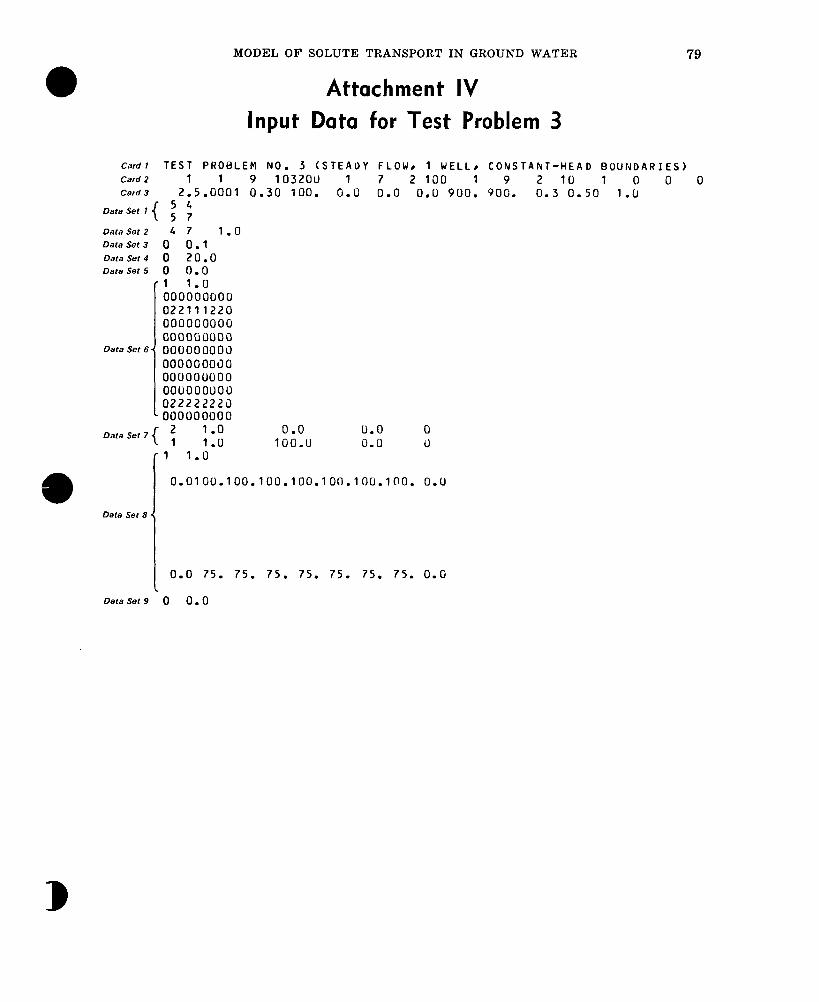
MODEL OF SOLUTE TRANSPORT IN GROUND WATER 79
Attachment IV
Input Data for Test Problem 3
cards TEST PROBLEM NO. 3 (STEADY FLOW, 1 WELLI CONSTANT-HEAD BOUNDARIES) Card 2 11 9 1032OU 1 7 2 100 1 9 2 IU 1 0 0 0 Card 3 2.5.0001 0.30 100. 0.0 0.0 0.0 900. 900. 0.3 0.50 l.u
Data Set 1 5 4 5 7
Data Set 2
Data Set 3
Data Set 4
Data Set 5
Data Set 6
47 1.0 0 0.1 0 20.0 0 0.0
-1 1.0 000000000 022111220 000000000 coootioooa 000000000 000000000 000000000 oouooouoo 022222223
- 000000000
Data Set 7 vi :i:
0.0 U.0 0 loo.u iJ.0 u
i
1 1.0
0.0100.100.100.100.100.1fl0.100. 0.1)
Data Set 8
I 0.0 75. 75. 75. 75. 75. 75. 75. 0.0
Data Set 9 0 0.0

80 TECHNIQUES OF WATER-RESOURCES INVESTIGATIONS
Attachment V
Selected Output for Test Problem 3
U.S.G.S. METHOD-OF-CHARACTERISTICS MODEL FOR SOLUTE TRANSPORT IN GROUND kATER
TEST PROBLEM ~0. 3 (STEADY FLowI 1 WELL, CONSTANT-HEAD ‘dOUhDARIES)
INPUT DATA
GRID DESCRIPTORS
NX (NUMBER OF COLUMNS) = 9 NY (NUMBER OF ROWS) = 10 XDEL (X-DISTANCE IN FEET) = 900.0 YDEL (Y-DISTANCE IN FEET) = 900.0
TIME PARAMLTERS
NTIM (MAX. NO. OF TIME STEPS) q
NPMP (NO. Of PUMPING PERIODS) = PINT (PUMPING PERIOD IN YEARS) = TIMX (TIME INCREMENT MULTIPLIER) = TINIT (INITIAL TINE STEP IN SEC.) =
HYDROLOGIC AND CHEMICAL PARAMETERS
S (STORAGE COEFFICIENT) = POROS (EFFECTIVE POROSITY) = BETA (CHARACTERISTIC LENGlHJ = DLTRAT (HAT10 OF TRANSVERSE TO
LONGITUDINAL DISPERSIVITY) = ANFClK (RATIO OF T-YY TO T-XX) =
EXECUTION PARAMETERS
NITP (NO. OF ITERATION PARAMETERS) = TOL CCONVEkGENCt CRITERIA - AOIPI =
1 1 2.50 0.00 0.
0.00000t 0.3u
100.0
0.30 1.000000
7 O.UOOl
I TMAX (MAx.N~.OF ITERATIoNs - ADIP) = 100 CELDIS CMAX.CELL DISTANCE PER M3VE
OF PAKTICLES - M.O.C.) NPMAX (MAX. NO. OF PARTICLES) NPTPND (NO. PARTICLES PER NODE)
PROGRAM OPTIONS
NPNT (TIME STEP INTERVAL FOR COMPLETE PRINTOUT) =
NPNTMV (MOVE INTERVAL FOR CHIM. CONCENTRATION PRINTOIJT) =
NPNTVL (PRINT OPTION-VELOCITY U=NO; l=FIRST TIME STEP; Z=ALL T‘IME STEPS) =
NPNTD CPKINT OPTION-DISP.COEF. O=NO; l=FIRST TLME STEP; 2=ALL TIME STEPS) I
NUMObS (NO. OF OHSERVATION WELLS FOR HYDROGRAPH PRINTOUT) 3
NREC (NO. OF PURPING WELLS) = NCODtS (FOR NODE IDENT.) = NPNCHV (PUNCH VELOCITIES) = NPDELC (PRINT OPT.-CONC. CHANGE) =
5 0.500 = 3200 = 9
1
10
1
0
2 1 2 0 0
c

MODEL OF SOLUTE TRANSPORT IN GROUND WATER 81
Selected output for test problem S-Continued
STEADY-STATE FLOW
TIME INTERVAL (IN SEC) FOR SdLUTE-TRANSPORT SIMULATION = 0.78894d+08
LOCATION OF OBSERVATION WELLS
NO. X Y
1 5 4
2 5 7
LOCATION OF PUkPING WELLS
x Y RATECIN CFS) CONC.
4 7 1.00 0.0
AREA OF ONE CELL = 0.8100d+06
X-Y SPACING: 900.00 9oc.00
TRANSMISSIVITY MAP (FT+FT/SEC)
0.00 0.00 0.00 0.00 0.00 0.00 0.00 0.00 0.00 0.00 0.10 0.10 0.10 0.10 0.10 0.10 0.10 0.00 0.00 0.10 0.10 0.10 0.10 0.10 0.10 0.10 0.00 0.00 0.10 O.lL 0.10 0.10 0.10 0.10 0.10 0.00
0.00 0.10 0.10 0.10 0.10 0.10 0.10 0.10 0.00 0.00 0.10 0.10 0.10 0.10 cl.10 0.10 0.10 0.00 0.00 0.10 0.10 0.10 0.10 0.10 0.10 0.10 0.00 0.00 Cl.10 0.10 0.10 0.10 0.10 0.10 0.10 0.00 0.00 0.10 0.10 0.10 0.10 0.10 0.10 0.10 0.00 0.00 0.00 0.00 0.00 0.00 0.00 0.00 0.00 0.00
AQUIFER THICKNESS (FT) 0.0 0.0 0.0 0.0 0.0 0.0 0.0 0.0 0.0
0.0 20.0 2o.c 20.0 20.0 20.0 20.0 20.0 0.0
0.0 20.0 20.0 20.0 20.0 20.0 20.0 20.0 0.0 0.0 20.0 20.0 20.0 20.0 20.0 20.0 20.0 0.0 0.0 20.0 20.0 20.0 20.0 20.0 20.0 20.0 0.0 0.0 20.0 20.0 20.0 20.G 20.0 20.0 20.0 0.0 0.0 20.0 20.0 20.0 20.0 20.0 20.0 20.0 0.0 0.0 20.0 2o.c 20.0 20.0 20.0 20.0 20.0 0.0 0.0 20.0 2O.O 20.0 20.0 20.0 20.0 20.0 0.0 0.0 0.0 0.0 0.0 0.0 0.0 0.0 0.0 0.0

82 TECHNIQUES OF WATER-RESOURCES INVESTIGATIONS
Selected output for test problem S-Continued
DIFFUSE RECHARGE AND 0 O.OOd+OU 0.000+00 O.OOd+OO 0.00d+00 O.OOd+OO 0.00a+00 O.OOdtOU 0.00at00 O.OOd+OO O.OOd+OO O.OOd+OO O.OOd+OO
U.OOd+OO O.OOd+OO O.OOd+OO O.OOd+OU
,ISCHARGE CFT/SEC) O.OOd+OO O.OOd+OO O.OOd+OO O.OOd+OO O.OOd+OO O.OOd+OO O.OOd+OO O.OOd+OO O.OOd+OO O.OOd+OO O.OOd+UO O.OOd+OO 0. UOd+OO O.OOd+OO O.OOd+OO O.OOd+OO O.GOd+OO O.OOd+OO O.OOd+OO O.OOd+OO
O.OOd+OO O.OOd+GO o.ood+oo 0.00c1+00 0.00d+00 o.3od+oo 0.00c1+00 o.ooc1+oo 0.00c1+00 0.00cl+00
0 .OOd+OO O.OOd+OO O.OOd+OO O.OOd+OO 0 .OOd+OO O.UOd+OO O.OOd+OO O.OOd+OO O.OOd+OO O.OOd+OO 0 .OOd+OO O.OOd+OO O.OOd+OO O.OOd+OO O.OOd+UO O.OOd+OO 0 .OOd+UO O.OOd*OO 0 .OOd+OO O.OOd+OO
PERMEABILTY MAP CFT/SEC) 0.0000.0000.0ll00.0U00.0000.0000.0000.0000.000 0.0000.0050.0050.0050.UU50.0050.0050.0050.00~~ 0.0000.0050.0050.0050.0050.0050.0050.0050.000 0.0000.0050.0050.0050.0050.0050.0050.000 0.0000.0050.0G50.0050.0050.U050~u050~005U.000 0.0000.0050.0050.0050.0050.0050.0050.0050.0050.00r1 0.0000.0050.0050.0050.0050.0050.0050.0050.0050.000 0.0000.0050.0050.0050.0050.0050.0050.0050.00U 0.0000.0050.0050.0050.0050.0050.0050.0050.000 0.0000.0000.0000.0000.00000.0000.0000.0000.000
NO. OF FINITE-DIFFERENCE CELLS IN AQUIFER = 56
AREA OF AQUIFER IN MODEL = 0.45360e+08 SQ. FT.
O.OOd+OO 3.30d+OO O.OOd+OO 0.30d+OO O.OOd+OO S.JOd+OO O.OOd+OO 0.30d+OO O.OOd+OO 0.3Dd*OO O.OOd+OO 0.3Dd+OO O,OOd+OO 0.30d+OO O.OOd+OO 0.30d+OO O.OOd+OO O.JOd+OO O.OOd+OO 3.33d+OO
NZCRIT (MAX. NO. OF CELLS THAT CAN HE VOID OF PARTICLES; IF EXCEEDED8 PARTICLES ARE REGENERATED) = 1
c

MODEL OF SOLUTE TRANSPORT IN GROUND WATER 83
Selected output for test problem %-Continued
NODE IDENTIFICATIOh MAP
0 0 0 0 0 0 0 0 0 0 2 2 1 1 1 2 2 0 0 u 0 0 0 0 0 0 u 0 0 0 0 0 0 0 0 0 0 0 0 0 0 0 0 0 0 0 0 0 0 0 0 0 0 0 0 0 0 0 0 0 0 0 0 0 0 0 0 0 0 0 0 0 0 2 2 2 2 2 2 2 0 0 u 0 0 0 0 0 0 0
NO. OF NODE IDENT. CODES SPECIFIED = 2
THE FOLLOWING ASSIGNMENTS HAVE BEEN MADE: CODE NO. LEAKANCE SOURCE CONC. RECHARGE
2 O.lOOe+bl 0.00
1 O.lOOe+Ol 100.00
VERTICAL PERMEABILITY/THICKNESS (FT/CFT*SEC)) 0.00 0.00 0.00 0.00 0.00 0.00 0.00 0.00 0.00 a.00 l.OrJ 1.00 1.00 1.00 1.00 1.00 1.00 0.00 0.00 0.00 0.00 0.00 0.00 0.00 0.00 0.00 0.00 0.00 0.00 0.00 0.00 0.00 0.00 0.00 0.00 0.00 0.00 0.00 o.cc 0.00 0.00 0.00 0.00 0.00 0.00 0.00 0.00 0.00 0.00 0.00 0.00 0.00 0.00 0.00 0.00 0.00 0.00 0.00 0.00 0.00 0.00 0.00
0.00 0.00
0.00 0.00 0.00 0.00 0.00 0.00 0.00 0.00 o.ao 1.00 1.00 1.00 1.00 1.00 1.00 1.00 0.00 0.00 0.00 0.00 0.00 0.00 0.00 0.00 0.00 0.00
WATER TAaLE 0. a. 0. 0. 0. 0. 100. 100. 100. 100. 0. cl. 0. 0. 0. 0. 0. 0. 0. 0. 0. 0. 0. 0. 0. 0. 0. 0. 0. 0. 0. 0. 0. “0: 2 0. 2 0. 75. 75. 7s. 75. 0. 0. 0. 0. 0.
0. 100.
0. 0. 0. 0. 0. 0.
75. 0.
0. 100.
0. 0. 0. 0.
ii: 75.
0.
0. 100. k
0. 0. 0. 0. 0. 0. 2 0. 0. 0”:
7s. 0. 0. 0.

84 TECHNIQUES OF WATER-RESOURCES INVESTIGATIONS
Selected output for test problem $-Continued
ITERATION PARAMETERS 0.246740a-01 0.4572994-01 0.8475394-01
157080 :291125 .539560 1 .ooooo
0.000000 0.000000 0.000000 0.000000 0.000000 0. ooooclo 0.000000 0.000000 0. C000C0 0.000000 0. ooooco 0.000000 0.000000
CONCENTRATION
NUMBER OF TIME STEPS = 0 TIME(SECONDS) = 0.00000
CHEM.TIME(SECONDS) = 0.00000e+00 CHEM.TIME(DAYS) = O.OOOOGe+OO
TIME(YEARS) = 0.00000e*00 CHEM.TIME(YEARS) = 0.00000e+00
NO. MOVES COMPLETED = 0
0 0 0 0 0 0
0 0 0 0 0 0
0 0 0 0 0 0
0 0 0 0 0 0
0 0 0 0 0 0
0 0 0 0 u 0
0 0 0 0 0 0
0 0 0 0 0 0
0 0 0 0 0 0
0 0 0 0 0 0
N = 1 NUMBER OF ITERATIONS = 20
0
0
Cl
0
0
0
0
0
0
0
0
0
0
0
0
0
0
0
0
0
0
0
0
0
0
0
0
0
0
0
c

MODEL OF SOLUTE TRANSPORT IN GROUND WATER 85
. : 4,
m
n ;: 00
:: 0
5:
8
d . 0
0 0
8 0
0” .
0
n
d
0 0 ,” z 0 ^’ . ,”
. 0
co
2 o- ,”
0
Fi
% h
0
2
0” z 8 8 z =: 0 0 . . 0
000000000
N . d .
2
0
0” 0
. 0 d

86 TECHNIQUES OF WATER-RESOURCES INVESTIGATIONS
0000000000 0000000000 l 0000000000 . . . . d 0’ 0’ 0’ 0’ d 0 0 0 0 QOQQOQQQQO QQQQQQOQQO 0000000000
d d d d d 0’ d 0. d d
0000000000 0000000000 0000000000 . . 0’ 0. d 0. 0 0 0’ d d 0’
rualuuuuu OtW*b*~h*tNO QrbNrOmOmO Ohu-.rNmmNNO
. . . . . . . . . . 000000Q000
8 I I 1 I I I I
ororeuuvuo OV\lcmr~lcmaJ0 Or.-tmNrN*r-OO oo.rcmnJ9rV\pco 0’ 0’ do’ d 0’ . . . . 0 0 0 0
c
2 0000000000 0000000000 0 0000000000
d ..*.......
0000000000 >
x
z 10000000000 0 0
2
2
0000000000 OQQOOOOOOO OqOOOOQOOO
. . . . . . . . . . OOOQOOOOOO

MODEL OF SOLUTE TRANSPORT IN GROUND WATER 87
0000000000 0000000000 0000000000 0’ do’ 0’ do’ 0’ 0’ 0’ 0’
0000000000 0000000000 0000000000
. . . . . . , , , , 0000000000
d 0’ d 0. 0. 0’ 0’ 0’ 0’ 0’
**.r.?**** 00000000 I I I I I I I , alouuYuoY
0o.o.mLnYlr000 ONNNrcorQNO O(clLrch~9mmO
0. 0’ 0. 0’ d 0’ 0. do’ d
0000000000
**G*ro.?< 0000000 I I I I , , , uuouuYo,
Orr-o.*thrmOo 0tnlnlc*0rr03 OrLr-~cors-M00 0’
0. 0’ . .
0 0’ 0. 0’ .
0 0’ 0
00000000 I I I I I I I I
: c
0000000000 0000000000 ;: 0000000000 0000000000 0000000000 0000000000 d
0. do’ 0. . . . .
0 0 d d 0 0 0. d 0. d 0’ 0’ 0. d 0’ 0’ > *
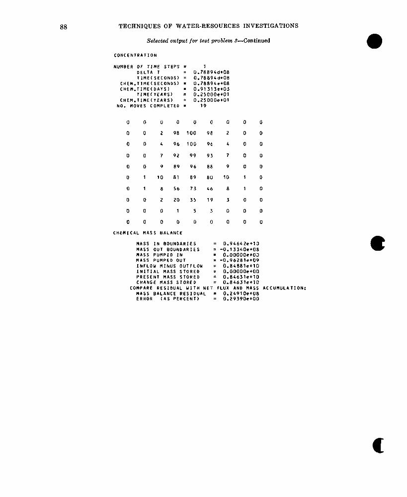
88 TECHNIQUES OF WATER-RESOURCES INVESTIGATIONS
Selected output for test problem 8-Continued
CONCENTRATION
NUMBER OF TIME STEPS = 1 DELTA T = 0.780944+u0 TlME( SECONDS) = 0.78894d+m
CHEM.TIMECSECONDS) = 0.78894et08 CHEM.TIME(DAYS) = 0.9131 Set03
TIME{ YEARS) = 0.25OOOe+Ol CHEM.TZME(YEARS) = 0.2SOOOe+Ol
NO. MOVES COMPLETED = 19
0 0
0 0
0 0
0 0
0 0
0 1
0 1
0 0
0 0
0 0
0 0 0 0
2 98 100 98
4 96 100 96,
7 92 99 9 3’
9 a9 96 0a*
10 81 89 80
8 56 73 4 6
2 20 35 1 5’
0 1 S 3;
0 0 0 Cl
CHEMICAL MASS BALANCE
MASS IN BOUNDARIES MASS OUT BOUNDARIES MASS PUMPED IN MASS PUMPED OUT
q
0 0 0
2 0 0
4 0 0
7 0 0
9 0 0
10 1 0
a 1 0
3 0 0
0 0 0
0 0 0
0.94642etlJ = -O.l334Oe*O8 = O.O0OOOe+O3 = -0.96201et09
INFLOU MINUS OUTFLOW = o.04aalet10 INITIAL MASS STORED = O.OO0OOe+OO PRESENT MASS STORED = 0.84631e+lO CHANGE MASS STORED = 0.84631e+?O
COMPARE RESIDUAL WITH NET FLUX AND MASS ACCUMULATION: MASS BALANCE RESIDUAL = 0.2491 Oe+U8 ERROR (AS PERCENT) = 0.29390etOO
c

MODEL OF SOLUTE TRANSPORT IN GROUND WATER
00000000~rrr.-.-.-rNNNN
2 ;I
L 00000000000000000300 . . . . . ..*............
OIXINNNNNNNNNNNNNNNNNN
2 mL300o-~~o-0m*o-c-Qa.o.o.00
w I
89

90 TECHNIQUES OF WATER-RESOURCES INVESTIGATIONS
*U.S. GOVERNMENT PRINTING OFFICE: 1978 O- 281-359459