A level set-based immersed interface method for solving incompressible viscous flows with the prescribed velocity at the boundary

INTERNATIONAL JOURNAL FOR NUMERICAL METHODS IN FLUIDSInt. J. Numer. Meth. Fluids 2010; 62:267–290Published online 26 February 2009 in Wiley InterScience (www.interscience.wiley.com). DOI: 10.1002/fld.2018

A level set-based immersed interface method for solvingincompressible viscous flows with the prescribed

velocity at the boundary

Zhijun Tan1,∗,†, K. M. Lim1,2 and B. C. Khoo1,2

1Singapore-MIT Alliance, 4 Engineering Drive 3, National University of Singapore, Singapore 117576, Singapore2Department of Mechanical Engineering, National University of Singapore, 10 Kent Ridge Crescent,

Singapore 119260, Singapore

SUMMARY

A second-order accurate immersed interface method (IIM) is presented for solving the incompressibleNavier–Stokes equations with the prescribed velocity at the boundary, which is an extension of the IIM ofLe et al. (J. Comput. Phys. 2006; 220:109–138) to a level set representation of the boundary in place ofthe Lagrangian representation of the boundary using control points on a uniform Cartesian grid. In orderto enforce the prescribed velocity boundary condition, the singular forces at the immersed boundary areapplied on the fluid. These forces are related to the jump in pressure and the jumps in the derivatives ofboth the pressure and velocity, and are approximated via using the local Hermite cubic spline interpolation.The strength of singular forces is determined by solving a small system of equations at each time step.The Navier–Stokes equations are discretized via using finite difference method with the incorporation ofjump conditions on a staggered Cartesian grid and solved by a second-order accurate projection method.Numerical results demonstrate the accuracy and ability of the proposed method to simulate the viscousflows in irregular domains. Copyright q 2009 John Wiley & Sons, Ltd.

Received 31 March 2008; Revised 12 January 2009; Accepted 16 January 2009

KEY WORDS: incompressible Navier–Stokes equations; singular force; immersed interface method;projection method; level set method; the prescribed velocity

1. INTRODUCTION

This paper concerns the viscous incompressible flows with the prescribed velocity condition atthe boundary. In a two-dimensional bounded domain D with the irregular boundary �D1 and

∗Correspondence to: Zhijun Tan, Singapore-MIT Alliance, 4 Engineering Drive 3, National University of Singapore,Singapore 117576, Singapore.

†E-mail: [email protected]

Copyright q 2009 John Wiley & Sons, Ltd.

268 Z. TAN, K. M. LIM AND B. C. KHOO

D

D2

D1 D1

D

D2

nX

x

s

y

Figure 1. A typical irregular domain (left) and the extended regular rectangular domain with an embeddedboundary (right) for the Navier–Stokes equations.

regular boundary �D2, the incompressible Navier–Stokes equations formulated in the primitivevelocity–pressure variables are considered and written as

�(ut +(u·∇)u)+∇ p=��u+Gext(x, t), x∈D (1)

∇ ·u=0, x∈D (2)

with initial and boundary conditions

u(x,0)=u0, u|�D1=up, u|�D2

=ub (3)

where u=(u,v)T is the fluid velocity, p is the fluid pressure, � is the fluid density, � is the fluidviscosity, x=(x, y) is the Cartesian coordinate variable, Gext(x, t)=(Gext

1 ,Gext2 )T is an external

forcing term. Throughout this paper, the fluid density � and fluid viscosity � are assumed to beconstants over the whole domain. The readers are referred to Figure 1 (left) for an illustration ofthe problem.

The irregular domain D can be extended to a larger rectangular domain � by an embeddingtechnique, see Figure 1 (right), where �+ =D and ��=�D2. In order to impose the prescribedvelocity condition at the irregular boundary, i.e. u|�D1

=up, the boundary �D1 can be treated as animmersed boundary � which exerts force to the fluid [1, 2]. These singular forces at the immersedboundary � can be introduced as the augmented variables so that the irregular boundary conditionis satisfied, i.e. u|� =up. The boundary � separates the extended fluid region into two parts �+and �− with �=�+∪�∪�−. Therefore, finding the solutions of Equations (1)–(3) is equivalentto solving the following equations:

�(ut +(u·∇)u)+∇ p=��u+Gext(x, t)+F(x, t), x∈� (4)

∇ ·u=0, x∈� (5)

u|� =up (6)

with the boundary condition u|�� =ub. Here, Equation (6) is the corresponding augmented equationand the singular force F has the form of

F(x, t)=∫

�f(s, t)�(x−X(s, t))ds (7)

Copyright q 2009 John Wiley & Sons, Ltd. Int. J. Numer. Meth. Fluids 2010; 62:267–290DOI: 10.1002/fld

LEVEL SET-BASED IIM FOR INCOMPRESSIBLE VISCOUS FLOWS 269

where X(s, t)=(X (s, t),Y (s, t)) is the arc-length parametrization of the boundary �, s is thearc-length, f=( f1, f2)T is the force density, and �(·) is the Dirac delta function defined in thedistribution sense. With the above embedding forcing approach, the original problem for (1)–(3)becomes an interface problem for (4)–(6) with a complete system on the regular domain. Thesolution in Equations (4)–(6) is a functional of the singular force f. For the current problems,the immersed boundary is rigid (i.e. the irregular boundary is fixed) and the velocity at therigid boundary is specified, then the singular force at the rigid boundary is determined by therequirement that the fluid velocity should satisfy the prescribed velocity at the rigid boundary,which is Equation (6).

Conventional methods for solving the Navier–Stokes equations with rigid immersed boundariesinclude the body-fitted or structured grid approach. In this approach, the Navier–Stokes equationsare discretized on a curvilinear grid that conforms to the immersed boundary and hence theboundary conditions can be imposed easily. The disadvantage of this method is that robust gridgeneration is required to account for the complexity of the immersed boundaries.

An alternative approach for solving complex viscous flows is the Cartesian grid method thatsolves the governing equations on a Cartesian grid and has the advantages of retaining the simplicityof the Navier–Stokes equations on the Cartesian coordinates and enabling the use of fast solvers.One of the most successful Cartesian grid methods is Peskin’s immersed boundary method [3].This method was originally developed to study the fluid dynamics of blood flow in the humanheart [4]. The method was further developed and has been applied to many biological problemsinvolving flexible boundaries [5, 6]. The immersed boundary method has also been applied tohandle problems with immersed boundaries [1, 7]. In order to deal with rigid immersed boundaries,Lai and Peskin [1] proposed to evaluate the force density using an expression of the form

f(s, t)=Kr (Xe(s)−X(s, t)) (8)

where Kr is a constant, Kr �1, X and Xe are the arc-parametrization of the computed and therequired positions of the boundaries, respectively. The forcing term in Equation (8) is a particularcase of the feedback forcing formulation proposed by Goldstein et al. [8] with �=0. In [8], theforce is expressed as

f(s, t)=�∫ t

0U(s, t ′)dt ′+�U(s, t) (9)

where U is the velocity of the boundary, and � and � are chosen to be negative and large enoughso that U will stay close to zero. In order to avoid using very small time step, Mohd-Yusof [9] andFadlun et al. [10] proposed a direct forcing formulation. This forcing is direct in the sense thatthe exact velocity is imposed directly on the rigid boundary through an interpolation procedure.Lima E Sliva et al. [7] proposed a different approach to compute the forcing term f based onthe evaluation of the various terms in the Navier–Stokes equations at the rigid boundary. Anothersimilar approach that combines the original immersed boundary method with the direct and explicitforcing was introduced by Uhlmann [11] for the simulation of particulate flows. The forcing termat the boundary is evaluated based on the desired velocity at the boundary, which is simply givenby the rigid-body motion and a preliminary velocity obtained explicitly without the application ofa forcing term.

Once the forcing term is obtained at the boundary, the immersed boundary method uses adiscrete delta function to spread the force density to the nearby Cartesian grid points. Since the



immersed boundary method smears out sharp interface to a thickness of order of the mesh widthand it is only first-order accurate for problems with non-smooth but continuous solutions. Incontrast, the immersed interface method (IIM) can avoid smearing out sharp interfaces and main-tains second-order accuracy by incorporating the known jumps into the finite difference schemenear the interface. The IIM was originally proposed by LeVeque and Li [12] for solving ellipticequations, and later extended to Stokes flow with elastic boundaries or surface tension [13]. Theinterested readers are referred to the newly published book by Li and Ito [14]. The method wasfurther developed for the Navier–Stokes equations in [15–17] for problems with flexible bound-aries. Recently, the IIM has been employed to solve for viscous flows with static rigid immersedboundaries [16, 18–20]. In [18, 19], the no-slip boundary conditions are imposed directly by deter-mining the correct jump conditions for stream function and vorticity. In [20], a Cartesian gridmethod for modeling multiple moving objects in incompressible viscous flow is considered. Leet al. [16] have presented an immerse interface method for viscous flows involving rigid and flexibleboundaries. In [16], the immersed boundaries are presented by a set of Lagrangian controls points.The strength of singular forces is determined to impose the no-slip condition at the boundary bysolving a small system of equations at each time step. Another Cartesian grid approach has beenpresented by Ye et al. [21] and Udaykumar et al. [22] via using a finite volume technique. Theyreshaped the immersed boundary cells and used a polynomial interpolating function to approxi-mate the fluxes and gradients on the faces of the boundary cells while preserving second-orderaccuracy.

In this work, a level set-based IIM with second-order accuracy is developed for solving theincompressible viscous flows with the prescribed velocity at the boundary, which is based onthe approach of Le et al. [16] in terms of the evaluation of the forcing term. The method combinesthe IIM with a level set representation of the interface on a uniform Cartesian grid, which is afurther extension of the work reported in [16] where the immersed boundary is represented bya cubic spline interpolation. However, the spline approach is difficult to use for multi-connecteddomains and for three-dimensional problems. In addition, the level set method usually has betterstability. For a spline approach, re-parameterization, filtering, and re-griding may be needed atevery or every other time steps. All these reasons favor a level set approach over a spline approach.The numerical implementation of the different interface representation avails the potential readera choice of the associated numerical techniques. In the proposed method, the singular force at theimmersed boundary is determined to enforce the prescribed velocity condition at the boundary.At each time step, the singular force is computed implicitly by solving a small, dense linearsystem of equations using singular value decomposition (SVD) iterative method. Once the forceis computed, next the jump in pressure and jumps in the derivatives of both the pressure andvelocity are computed. The Navier–Stokes equations are discretized on a staggered Cartesian gridby a second-order accurate projection method for the pressure and velocity. The jumps in thesolution and its derivatives are incorporated into the finite difference discretization to obtain asharp interface resolution. Fast solvers from the FISHPACK software library [23] are used to solvethe resulting discrete systems of equations. The numerical results show that the overall scheme issecond-order accurate for the velocity and nearly second-order accurate for the pressure.

The rest of the paper is organized as follows. In Section 2, the jump conditions for the velocity andpressure and their derivatives along the immersed boundary via the singular force f are presented.The numerical algorithm and numerical implementation are presented in Sections 3 and 4,respectively. In Section 5, some numerical examples are presented. Some concluding remarks willbe made in Section 6.



2. JUMP CONDITIONS ACROSS THE BOUNDARY

With the singular force, the jump conditions for the solutions of the Navier–Stokes equationsand their derivatives can be applied and determined. Let n=(n1,n2) and s=(�1,�2) be the unitoutward normal and tangential vectors to the boundary �, respectively. The jump of an arbitraryfunction q(X) across � at X is denoted by

[q]= lim�→0+ q(X+�n)− lim

�→0+ q(X−�n) (10)

Denoting (,) the local coordinates associated with the directions of n and s, respectively, thejump conditions for the velocity and pressure (see [15, 16] for details) are as follows:

[u]=0, [u]=0, [u]=−1

�f̂2s (11)

[u]= 1

�� f̂2s, [u]=−1

�

� f̂2�s− 1

�� f̂2n (12)

[u]=−[u]+ 1

�[p]n+ 1

�[p]s− 1

�[Gext] (13)

[p]= f̂1, [p]=[Gext]·n+ � f̂2�

, [p]= � f̂1�

(14)

[p]= �2 f̂1�2

−�[p], [p]= �([Gext]·n)

�+ �2 f̂2

�2+�[p] (15)

[p]=[∇ ·Gext]+v[u]−u[v]−[p] (16)

Here, f̂1 and f̂2 are the components of the force density in the normal and tangential directions ofthe embedded boundary, denoting f̂=( f̂1, f̂2), and � is the curvature of the embedded boundary. Inthis work, the jump conditions of second-order spatial derivative for the pressure are incorporatedinto the finite difference scheme. It is noted from expressions (11)–(16) that the values of thejumps of the first and second-order derivatives of the velocity and pressure taken with respect tothe (x, y) coordinates are easily obtained by a simple coordinate transformation:

[qx ]=[q]n1+[q]�1, [qy]=[q]n2+[q]�2 (17)

[qxx ]=[q]n21+2[q]n1�1+[q]�21 (18)

[qyy]=[q]n22+2[q]n2�2+[q]�22, q=u, p (19)

3. NUMERICAL ALGORITHM

The numerical algorithm to be employed is based on the pressure-increment projection algorithmfor the discretization of the Navier–Stokes equations with special treatment at the grid points nearthe embedded boundary [16]. The spatial discretization is carried out on a standard marker-and-cell



,i jp,i ju

,i jv

p

, 1i jv

1,i j

1,i j

u

Figure 2. A diagram of the embedded boundary cutting through a staggered grid with a uniform meshwidth h, where the velocity component u is at the left–right face of the cell and v is at the top–bottom

face, and the pressure is at the cell center.

(MAC) staggered grid similar to that found in Harlow and Welch [24]. A uniform MAC gird withmesh width h=�x=�y is used in the computation. With the MAC mesh, the pressure field isdefined at the cell center (i, j), where i ∈{1,2, . . . ,Nx } and j ∈{1,2, . . . ,Ny}. The velocity fieldsu and v are defined at the vertical edges and horizontal edges of a cell, respectively. The pressureand the velocity components u and v are arranged as in Figure 2.

3.1. Projection method

Assuming that the force f at the immersed boundary is known, the pressure-increment procedurefor problems with immersed interfaces is analogous to the projection method presented in [25].The discretization of the Navier–Stokes equations at those grid points near the embedded boundaryneeds to be modified to account for the jump conditions across the boundary due to the presenceof singular forces at the boundary. The discreted expressions will include coefficients C1, C2, etc.,which will be evaluated later. Given the velocity un and the pressure pn−1/2, the velocity un+1

and pressure pn+1/2 at the next time step are computed as follows:Step 1: Compute an intermediate velocity field u∗ by solving

u∗−un

�t+(u·∇u)n+1/2=−1

�∇ pn+1/2+ �

2�(�hu∗+�hun)+ 1

�gn+1/2+C1 (20)

u∗|�� =un+1b (21)

where the advection term is extrapolated using the formula

(u·∇u)n+1/2= 32 (u·∇hu)n− 1

2 (u·∇hu)n−1+C2 (22)

and the pressure gradient is approximated simply as

∇ pn+1/2=GMAC pn−1/2+C3 (23)



The above step can be rewritten in the following Helmholtz equations form:

�0u∗+�hu∗ =RHS (24)

where RHS is the right hand, which includes the correction terms and �0=−2�/��t .Step 2: Compute a pressure update n+1 by solving the Poisson equation

�h n+1= �

�tDMACu∗+C4 (25)

with boundary condition

n·∇ n+1|�� =0

Step 3: Once n+1 is obtained by solving Equation (25), both the pressure and velocity field(pn+1/2,un+1) are updated as

un+1=u∗− �t

�GMAC n+1+C5 (26)

pn+1/2= pn−1/2+ n+1− �

2�DMACu∗+C6 (27)

The coefficients C1,C2,C3,C4,C5, and C6 are the spatial correction terms, which are added tothe finite difference equations at the points near the boundary to improve the accuracy of the localfinite difference approximations. These correction terms can be computed by using the generalizedfinite difference formulas if the jumps in the solution and their derivatives are known and will beevaluated later. In the above expressions, ∇h and �h are the standard central difference operators,GMAC and DMAC are the MAC gradient and divergence operators, respectively. These operatorsare defined as

∇hui, j =(ui+1, j −ui−1, j

2h,ui, j+1−ui, j−1

2h

)(28)

�hui, j = ui+1, j +ui−1, j +ui, j+1+ui, j−1−4ui jh2

(29)

(GMAC p)i j =(pi+1, j − pi, j

h,pi, j+1− pi, j

h

)(30)

(DMACu)i, j = ui+1, j −ui, jh

+ vi, j+1−vi, j

h(31)

In our projection method, two Helmholtz equations for u∗ in (21) or (24) and one Poisson-likeequation for n+1 in (25) need to be solved at each time step. Since the correction terms in (21)or (24) and (25) only affect the right-hand sides of the discrete systems for the Helmholtz andPoisson equations, there are many methods which can be used to solve these linear system, forexample, the conjugate gradient method and multigrid method. In the present work, the fast solversfrom FISHPACK [23] are used to solve these equations.



3.2. Correction terms calculation

In this section, the correction terms C1, C2, C3, C4, C5, and C6 will be evaluated. One ofthe basic components for determining the correction terms is the generalized finite differenceformulas which will be briefly reviewed in this section. Here four generalized finite differenceformulas are shown for demonstration. Assume that the boundary cuts a grid line between twogrid points at x=�, xi��<xi+1, xi ∈�−, xi+1∈�+, where �− and �+ denote the region insideand outside the boundary, respectively. Then, the following approximations hold for a piecewisetwice differentiable function q(x):

qx (xi )= qi+1−qi−1

2h− 1

2h

2∑m=0

(h+)m

m! [q(m)]�+O(h2) (32a)

qxx (xi )= qi+1−2qi +qi−1

h2− 1

h2

2∑m=0

(h+)m

m! [q(m)]�+O(h) (32b)

where q(m) denotes the mth derivative of q, qi =q(xi ), h+ = xi+1−�, h− = xi −� and h is themesh width in x direction. The jump in q and its derivatives are defined as

[q(m)]� = limx→�,x∈�+ q

(m)(x)− limx→�,x∈�− q

(m)(x) (33)

in short, [·]=[·]�, and q(0) =q . Note that if the boundary cuts a grid line between two grid pointsxi ∈�+ and xi+1∈�−, these expressions need to be modified by changing the sign of the secondterms on the respective right-hand sides. Expressions involving two or more boundary crossingscould also be derived, the readers are referred to [26] for details. From Equations (32a) and (32b)the correction terms for qx (xi ) and qxx (xi ) can be defined as

C{qx (xi )}=− 1

2h

2∑m=0

(h+)m

m! [q(m)] (34)

C{qxx (xi )}=− 1

h2

2∑m=0

(h+)m

m! [q(m)] (35)

Thus, the finite difference approximation near the boundary, for the derivatives of a function q ,includes the standard central difference terms plus the additional correction terms. Accordingly,the correction terms C1, C2, C3, C4, C5 and C6 are evaluated as follows:

C1= 1

2�(C{�u∗}+C{�un}) (36a)

C2= 32C{(u·∇u)n}− 1

2C{(u·∇u)n−1} (36b)

C3=C{∇ pn−1/2} (36c)

C4=�C{∇ ·u∗}

�t−C{∇(∇ pn+1/2)}+C{∇(∇ pn−1/2)} (36d)



C5=−�t

�(C{∇ pn+1/2}−C{∇ pn−1/2}) (36e)

C6=− �

2�C{∇ ·u∗} (36f)

It is noted that all the correction terms are evaluated at least for first-order accuracy. This issufficient to guarantee second-order accuracy globally since our numerical scheme is second orderaway from the boundary and only the irregular points near the boundary are treated with a first-order scheme. In (36a), (36d), and (36f ), the jump conditions for un+1 are used to approximatethe jump conditions for u∗ as it is expected that u∗ is a good approximation for un+1. To evaluatethe correction term C{�u∗} of (36a) at a point (i, j) as depicted in Figure 3, [u∗

x ] and [u∗xx ] at the

intersection point �, and [u∗y] and [u∗

yy] at � using the force strength at time level n+1 need to becomputed. The correction term C{�u∗} is calculated as follows:

C{�u∗}i, j =−[u∗]+h+[u∗

x ]�+ (h+)2

2[u∗

xx ]�h2

−[u∗]+k−[u∗

y]�+ (k−)2

2[u∗

yy]�h2

where h+ = xi+1−x�, k− = y j−1− y�, and x� and y� are the x-coordinate of the intersection point� and the y-coordinate of the intersection point � as shown in Figure 3, respectively. �u∗ isapproximated at the irregular point (i, j) as

�u∗(i, j)=�hu∗i, j +C{�u∗}i, j +O(h)

Similarly, other correction terms in (36b)–(36f ) can be computed as follows:

C{∇ ·u}i, j =−[u]+h+[ux ]�+ (h+)2

2[uxx ]�

h+

[v]+k−[vy]�+ (k−)2

2[vyy]�

h

C{∇ p}i, j =

⎛⎜⎜⎝−

[p]+h+[px ]�+ (h+)2

2[pxx ]�

h,

[p]+k−[py]�+ (k−)2

2[pyy]�

h

⎞⎟⎟⎠

(i, j)

Irregular grid pointRegular grid point

Figure 3. The embedded boundary and mesh geometry near the irregular grid point (i, j).



3.3. Level set representation of boundaries

The zero level set of a two-dimensional function �(x, y) is used to represent the boundary. Thatis, �(x, y) is such a function such that

�={(x, y) :�(x, y)=0} (37)

Generally, �(x, y) is chosen as the signed distance function from the boundary.�+ ={(x, y), |�(x, y)�0} and �− ={(x, y), |�(x, y)<0} are denoted. In this work, the levelset function is defined at the same location with the pressure (at the cell center), i.e �i, j =�(xi+1/2, y j+1/2). A grid point (xi+1/2, y j+1/2) is called an irregular inner grid point if �i, j<0and any of the following four inequalities is true:

�i, j ·�i−1, j � 0, �i, j ·�i+1, j�0

�i, j ·�i, j−1 � 0, �i, j ·�i, j+1�0(38)

Similarly, a grid point (xi+1/2, y j+1/2) is an irregular outer grid point if �i, j�0 and any of thefollowing four inequalities is true:

�i, j ·�i−1, j < 0, �i, j ·�i+1, j<0

�i, j ·�i, j−1 < 0, �i, j ·�i, j+1<0(39)

Then the projection points {X∗}={(X∗,Y ∗)} of the irregular grid points onto the boundaryare computed, as illustrated in Figure 4. Assume that xi+1/2, j+1/2 is an irregular grid point. Thecorresponding orthogonal projection point on the boundary satisfies

X∗ =xi+1/2, j+1/2+�w (40)

where w=(��i j/�x,��i j/�y). Using the Taylor expansion of �(X∗)=�(xi j +�w)=0 at xi j , thefollowing quadratic equation for the unknown variable � is obtained:

�i j +(∇�i j ·w)�+ 12 (w

TH(�i j )w)�2=0 (41)

(xi+1/2 , yj+1/2)

(xi+1/2 , yj+3/2)

(xi+3/2 , yj+1/2)

(xi+3/2 , yj+3/2)

Y *

X *

Figure 4. The corresponding projection point X∗ =(X∗,Y ∗) of an irregular grid point x=(xi , y j ) on theboundary �, where (,) is the local coordinate system at X∗.



where the Hessian matrix H is defined as

H(�i j )=

⎛⎜⎜⎜⎜⎜⎝

�2�i j

�x2�2�i j

�x�y

�2�i j

�y�x

�2�i j

�y2

⎞⎟⎟⎟⎟⎟⎠ (42)

The detailed algorithm for finding the projection points is explained in [27, 28]. The spatialderivatives of the level set function are approximated using the following central finite differenceschemes at (xi+1/2, y j+1/2):

��i j

�x≈ �i+1, j −�i−1, j

2h,

��i j

�y≈ �i, j+1−�i, j−1

2h(43)

�2�i j

�x2≈ �i+1, j −2�i, j +�i−1, j

h2,

�2�i j

�y2≈ �i, j+1−2�i, j +�i, j−1

h2(44)

�2�i j

�x�y= �2�i j

�y�x≈ �i+1, j+1+�i−1, j−1−�i+1, j−1−�i−1, j+1

4h2(45)

At each orthogonal projection point X∗, the geometrical information needed includes the curvature� and the angle � between the normal direction and the x-axis at X∗. The curvature is defined asusual

�=−�2��x2

(��

�y

)2

−2�2��x�y

��

�x��

�y+ �2�

�y2

(��

�x

)2

((��

�x

)2

+(

��

�y

)2)3/2

(46)

The unit normal direction is determined by

n1=��

�x√(��

�x

)2

+(

��

�y

)2, n2=

��

�y√(��

�x

)2

+(

��

�y

)2(47)

The derivatives of � at X∗ can be approximated using the bilinear interpolation formula from thederivatives already calculated at four neighboring grid points using (43)–(45). Similarly, � and nat X∗ can be calculated.

3.4. Calculation of surface derivatives

To determine the above correction terms (36a)–(36f ), a key part is to compute the first and secondderivatives of the force f along the boundary. It is assumed that the values of the boundary function (s) are known at all the projection points {X∗

K } from the inner irregular grid points and below is



K-1

K-2

K+1K+2

( , )x y

Figure 5. A diagram used to interpolate the surface derivatives at the intersections of the boundary � andgrid lines, where dark circles represent the projection points from the inner irregular grid points.

how to interpolate (s), ′(s), and ′′(s) at the intersections of the boundary and grid lines, and ′(s) and ′′(s) at the projection points from the inner irregular grid points, see Figure 5 for anillustration. The least-squares interpolation scheme for approximating (s∇) can be written as∑

k�k (sk) (48)

where �k’s are the coefficients, which need to be determined from the Taylor expansion at theinterpolation point s∇

(sk)= (s∇)+ ′(s∇)�sk+ 12

′′(s∇)(�sk)2+O((�sk)

3) (49)

where �sk =sk −s∇ is the signed arc-length from the boundary point at s=sk to the point ats=s∇ . Defining

a1=∑k

�k, a2=∑k

(sk−s∇)�k, a3=∑k

12 (sk−s∇)2�k (50)

and substituting (49) into (48), the coefficients �k can be obtained by setting

a1=1, a2=0, a3=0 (51)

In order to keep the symmetry strictly, in our computations, the first closest two projection points tothe intersection point (X (s∇),Y (s∇)) from each side of this point are chosen for the interpolation,respectively, then the SVD method is used to solve the system of equations (51). Similarly, othersurface derivatives ′(s∇) and ′′(s∇) can be obtained.

3.5. Determination of force f at projection points

If the force f at the immersed boundary is known as assumed before, the velocity field un+1 atall the grid points can be computed via the projection method as discussed in Section 3.1. Thevelocity at the projection points from the outside of the boundary, Uk , can be interpolated fromthe velocity un+1 at the grid points as in [16]. Thus, it can be written as

Uk =U(Xk)=I(un+1) (52)



where I is the interpolation operator that includes the appropriate correction terms required toguarantee at least second-order accuracy when the derivatives of the velocity are discontinuous.Two ways are to use the third-order accurate least-square interpolation scheme in [14] and themodified bilinear interpolation with jump conditions in [16]. As an alternative approach, threenearby points are used to perform linear interpolation that is modified to incorporate the jumpcondition at the boundary. The readers are referred to [13] for details. Since the relationshipsbetween the singular forces and the jumps in the solution or its derivatives are linear and all theimplicit equations solved at each time step of the projection method are linear, the velocity at theimmersed boundary can be written as

Uk =U0k+Af (53)

where U0k corresponds to the velocity at the projection points obtained by solving Equations (4)

and (5) with f=0, given un and pn−1/2. A is a 2Nb×2Nb matrix, where Nb is the number ofprojection points. The vector Af is the velocity at the projection points obtained by solving thefollowing equations:

u∗f

�t= �

2��hu∗

f +C̄1, u∗f |�� =0 (54)

�h n+1f = �

�tDMACu∗

f +C̄4, n·∇ n+1f |�� =0 (55)

un+1f =u∗

f − �t�

�GMAC n+1

f +C̄5 (56)

Af=I(un+1f ) (57)

with f being the singular force at the immersed boundary. Here, C̄1, C̄4, and C̄5 are the correctionterms that take into account the effect of the singular force f at the immersed boundary. FromEquation (53), with the prescribed velocity Up at the immersed boundary, the singular force f atthe immersed boundary is determined by solving

Af=Up−U0k (58)

Note that the matrix A depends on the location of the boundary and the time step �t . If theboundary and the time step are fixed, the matrix A will be same at every time step. Therefore,the matrix A needs to be formed and factorized only once in this case. In order to compute thecoefficients of A, Equations (54)–(56) are solved for 2Nb times, i.e. once for each column. Eachtime, the singular force f is set to zero except for the entry corresponding to the column that isto be calculated, which is set to one. Once the matrix A has been calculated, only the terms onthe right-hand side, Up−U0

k , need to be computed at each time step. The resulting small systemof Equation (58) is then solved at each time step for f via back substitution. Finally, Equations(21)–(27) are solved to obtain un+1 and pn+1/2. In actual computation, the SVD method is usedto solve the system of Equation (58).



4. NUMERICAL IMPLEMENTATION

In this section, a basic implementation of the proposed algorithm is described. The coefficientmatrix using SVD is factorized as

A=URVT (59)

where U=[u1, . . . ,uNb ] and V=[v1, . . . ,vNb ] are orthogonal matrices and R=diag(�1, . . . ,�Nb)

is a diagonal matrix whose elements are the singular values of the original matrix such that

�1��2� · · ·��Nb�0 (60)

U,V, and R are stored for solving the force f at every time step. At each time step, given thevelocity field un and pressure field pn−1/2, the proposed algorithm for finding un+1, pn−1/2,and the singular force f to enforce the prescribed velocity Up at the immersed boundary can besummarized as follows:

Algorithm The implementation of the IIM with the prescribed velocity at the boundary

Step 1: Compute the right-hand side of (58) by calculating Up−U0k .

• Set f=0, and solve (24)–(26) for the velocity at all the grid points.• Interpolate the velocity at the projection points U0

k as in (52).• Compute the right-hand side vector b=Up−U0

k .

Step 2: Compute the singular force f by solving (58) using the SVD method. The singular forcef can be written in terms of the SVD as

w=Nb∑i=1

uTi b

�ivi (61)

Step 3: Compute un+1 and pn+1/2 using the projection method with the incorporation of theappropriate correction terms.

5. NUMERICAL EXAMPLES

In this section, several numerical experiments are carried out to demonstrate the capabilities andthe accuracy of the proposed algorithm in this work. Throughout this section, � is taken to be 1in all simulations.

Example 5.1 (Circular Couette flow)In the first example, the steady circular Couette flow between two rotating translating concentriccylinders is considered. The domain of the simulation and the geometry of the two rotatingconcentric cylinders are shown in Figure 6. The solution domain is the rectangle of the size[−ax/2,ax/2]×[−bx/2,bx/2]. The angular velocities of the inner and outer cylinders are denoted



r1

r2

1

2

ax

ay

x

y

Figure 6. The domain of the simulation and the geometry of circular Couette flow.

as �1 and �2, respectively. In the simulations, r1=0.5, r2=2.0, ax =ay =2. The analyticalsolution of the steady flow between the two cylinders is given by

u=−(A+ B

r2

)y (62)

v=(A+ B

r2

)x (63)

p= A2r2

2− B2

2r2+AB ·ln(r2)+ p0 (64)

where r =√x2+ y2, p0 is an arbitrary constant, and A1 and A2 are

A= �2r22 −�1r21r22 −r21

(65)

B= (�1−�2)r21r22

r22 −r21(66)

The Dirichlet boundary conditions are applied for the velocity at the far-field boundary �� inFigure 6, and they are obtained from the analytical solution. In the current numerical setup, onlythe inner cylinder � is contained in the simulation domain. It is easy to verify that the velocitysatisfies the incompressibility constraint, and it is continuous but has a finite jump in the normaldirection across the boundary.

In our computations, the simulation is performed with a 64×64 grid, and the time step is takenas �t=�x/4. We first take �1=1, �2=−1, and �=0.1. In Figure 7, the plots for the computedu-component velocity and the velocity field at t=10 are presented. From Figure 7(a), it can beseen that the velocity u is continuous but not smooth, as expected. In this case, the grid refinement



0

0.5

1

0

y

x0.5

1

0

0.5

1

u

0 0.2 0.4 0.6 0.8 1

0

0.2

0.4

0.6

0.8

1Velocity field at t = 10

(a) (b)

Figure 7. For Example 5.1 on circular Couette flow: (a) the x-component of velocity field u and (b) thevelocity field u with �1=1,�2=−1 and �=0.1 at t=10.

00.5

10y

x

0.5

1

0

0.1

0.2

0.3

P

Figure 8. For Example 5.1 on circular Couette flow. Pressure distributionwith �1=1,�2=−1 and �=0.1 at t=10.

analysis is performed to determine the order of convergence of the algorithm. The order of accuracyis estimated as (Figure 8)

order= log(‖Eu(N )‖∞ /‖Eu(2N )‖∞)

log2(67)



Table I. Grid refinement analysis for Example 5.1 with �1=1,�2=−1 and �=0.1 at t=2.

N ‖Eu ‖∞ Order ‖Ep ‖∞ Order

32 1.2114E−02 — 1.5329E−02 —64 2.7106E−03 2.16 4.1359E−03 1.89128 6.5912E−04 2.04 1.1315E−03 1.87256 1.5698E−04 2.07 3.0108E−04 1.91

here, ‖Eu(N )‖∞ is the maximum error

‖Eu(N )‖∞=maxi, j

|Ui j −u(xi , y j )| (68)

where u(xi , x j ) is the exact solution at (xi , x j ) and Ui j is the numerical solution.The result of the convergence rate analysis is shown in Table I. From Table I, one can easily see

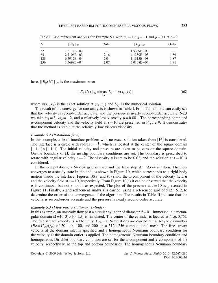
that the velocity is second-order accurate, and the pressure is nearly second-order accurate. Nextwe take �1=2, �2=−2, and a relatively low viscosity �=0.001. The corresponding computedu-component velocity and the velocity field at t=10 are presented in Figure 9. It demonstratesthat the method is stable at the relatively low viscous viscosity.

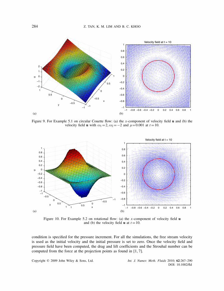
Example 5.2 (Rotational flow)In this example, a fixed interface problem with no exact solution taken from [16] is considered.The interface is a circle with radius r = 1

2 , which is located at the center of the square domain[−1,1]×[−1,1]. The initial velocity and pressure are taken to be zero on the square domain.On the boundary of �, the no-slip boundary conditions are set. The boundary is prescribed torotate with angular velocity �=2. The viscosity � is set to be 0.02, and the solution at t=10 isconsidered.

In the computations, a 64×64 grid is used and the time step �t=�x/4 is taken. The flowconverges to a steady state in the end, as shown in Figure 10, which corresponds to a rigid-bodymotion inside the interface. Figures 10(a) and (b) show the x-component of the velocity field uand the velocity field at t=10, respectively. From Figure 10(a) it can be observed that the velocityu is continuous but not smooth, as expected. The plot of the pressure at t=10 is presented inFigure 11. Finally, a grid refinement analysis is carried, using a referenced grid of 512×512, todetermine the order of the convergence of the algorithm. The results in Table II indicate that thevelocity is second-order accurate and the pressure is nearly second-order accurate.

Example 5.3 (Flow past a stationary cylinder)In this example, an unsteady flow past a circular cylinder of diameter d=0.1 immersed in a rectan-gular domain �=[0,3]×[0,1.5] is simulated. The center of the cylinder is located at (1.6,0.75).The free stream velocity is set to unity, U∞ =1. Simulations are carried out at Reynolds number(Re=U∞d/�) of 20, 40, 100, and 200 on a 512×256 computational mesh. The free streamvelocity at the domain inlet is specified and a homogeneous Neumann boundary condition forthe velocity at the domain outlet is applied. The homogeneous Neumann boundary condition andhomogeneous Dirichlet boundary condition are set for the x-component and y-component of thevelocity, respectively, at the top and bottom boundaries. The homogeneous Neumann boundary



0

x

0.5

1

0

y

0.5

(a) (b)

1

0

1

2

u

0 0.2 0.4 0.6 0.8 1

0

0.2

0.4

0.6

0.8


Figure 9. For Example 5.1 on circular Couette flow: (a) the x-component of velocity field u and (b) thevelocity field u with �1=2,�2=−2 and �=0.001 at t=10.

0x

0.51

0

y 0.51

(a) (b)

0

0.2

0.4

0.6

0.8

1

u

0 0.2 0.4 0.6 0.8 1

0

0.2

0.4

0.6

0.8


Figure 10. For Example 5.2 on rotational flow: (a) the x-component of velocity field uand (b) the velocity field u at t=10.

condition is specified for the pressure increment. For all the simulations, the free stream velocityis used as the initial velocity and the initial pressure is set to zero. Once the velocity field andpressure field have been computed, the drag and lift coefficients and the Strouhal number can becomputed from the force at the projection points as found in [1, 7].



0

x

0.510

y

0.5

1

0

0.1

0.2

P

Figure 11. For Example 5.2 on rotational flow. Pressure distribution at t=10.

Table II. Grid refinement analysis for Example 5.2 with �=0.02 at t=10.

N ‖Eu ‖∞ Order ‖Ep ‖∞ Order

64 1.6705E−03 — 5.3145E−03 —128 4.3235E−04 1.95 1.4044E−03 1.92256 1.0155E−04 2.09 3.8421E−04 1.87

1.45 1.5 1.55 1.6 1.65 1.7 1.75 1.8 1.85 1.9 1.950.6

0.65

0.7

0.75

0.8

0.85

0.9Re = 20: Streamlines

Figure 12. For Example 5.3 on flow past a stationary cylinder. Streamlines for Re=20.

The plots of streamline for Re=20 and Re=40 at steady state are shown in Figures 12 and 14,respectively. For these low Reynolds numbers, as expected, the flow gradually attains a steady stateand the wake forms behind the cylinder symmetrically. In Figures 13 and 15, the correspondingplots of the pressure contours for Re=20 and Re=40 are also shown, respectively. These results



Re = 20: Pressure contours

1 1.2 1.4 1.6 1.8 2 2.2 2.4 2.6 2.8 30.3

0.4

0.5

0.6

0.7

0.8

0.9

1

1.1

1.2

Figure 13. For Example 5.3 on flow past a stationary cylinder. Pressure contours for Re=20.

1.45 1.5 1.55 1.6 1.65 1.7 1.75 1.8 1.85 1.9 1.950.6

0.65

0.7

0.75

0.8

0.85

0.9Re = 40: Streamlines

Figure 14. For Example 5.3 on flow past a stationary cylinder. Streamlines for Re=40.


1 1.2 1.4 1.6 1.8 2 2.2 2.4 2.6 2.8 30.3

0.4

0.5

0.6

0.7

0.8

0.9

1

1.1

1.2

Figure 15. For Example 5.3 on flow past a stationary cylinder. Pressure contours for Re=40.



Table III. Length of the recirculation zone (L/d) and drag coefficient (CD) for Re=20 and Re=40.

Re=20 Re=40

L/d CD L/d CD

Tritton [31] — 2.22 — 1.48Coutanceau and Bouard [30] 0.73 — 1.89 —Fornberg [29] 0.91 2.00 2.24 1.50Calhoun [18] 0.91 2.19 2.18 1.62Russell and Wang [20] 0.94 2.13 2.29 1.60Ye et al. [21] 0.92 2.03 2.27 1.52Le et al. [16] 0.93 2.05 2.22 1.56Present 0.93 2.06 2.24 1.57


1 1.2 1.4 1.6 1.8 2 2.2 2.4 2.6 2.8 30.3

0.4

0.5

0.6

0.7

0.8

0.9

1

1.1

1.2


1 1.2 1.4 1.6 1.8 2 2.2 2.4 2.6 2.8 30.3

0.4

0.5

0.6

0.7

0.8

0.9

1

1.1

1.2

Figure 16. For Example 5.3 on flow past a stationary cylinder. Pressurecontours for Re=100 and Re=200.

are found in a very good agreement with the results of [16]. At the steady state, the drag coefficientsand the length of the recirculation zone are computed and are compared with other numericalresults [7, 16, 18, 20, 21, 29] as well as experimental results [30, 31] in Table III. It is clear that ourdrag coefficients are in reasonably good agreement with them. At Re=100 and Re=200, the flowis unsteady, and Figure 16 shows the pressure field at Re=100 and Re=200. The instability andvortex shedding can be seen from this figure. In Table IV, the drag coefficients, lift coefficients,



Table IV. Summary of results for Re=100 and Re=200.

Re=100 Re=200

CL CD St CL CD St

Braza et al. [32] ±0.250 1.36±0.015 — ±0.75 1.40±0.050 —Liu et al. [33] ±0.339 1.35±0.012 0.164 ±0.69 1.31±0.049 0.192Calhoun [18] ±0.298 1.33±0.014 0.175 ±0.67 1.17±0.058 0.202Russell and Wang [20] ±0.300 1.38±0.007 0.169 ±0.50 1.29±0.022 0.195Le et al. [16] ±0.323 1.37±0.009 0.160 ±0.43 1.34±0.030 0.187Present ±0.329 1.37±0.010 0.162 ±0.56 1.36±0.040 0.193

0 50 100 150 200 250 300 350 400 450 5001.1

1.15

1.2

1.25

1.3

1.35

1.4

1.45

1.5

T0 50 100 150 200 250 300 350 400 450 500

T

CD

CL 0

0.1

0.2

0.3

0.4

Figure 17. For Example 5.3 on flow past a stationary cylinder. Drag andlift coefficients versus time for Re=100.

and Strouhal numbers at Re=100 and Re=200 are compared with other numerical results. Goodagreement is again found from this table. In particular, the plots of time evolution of the drag andlift coefficients at Re=100 are presented in Figure 17.

6. CONCLUDING REMARKS

In this paper, a level set-based immersed interface algorithm is presented for solving the incompress-ible Navier–Stokes equations with the prescribed velocity at the boundary. The method combinesthe IIM with a level set representation of the interface on a uniform Cartesian grid. The mainadvantage of the method is that the prescribed boundary condition is exactly satisfied. The gridconvergence analysis shows that current algorithm can achieve second-order accurate in both thevelocity and pressure. It is a rather straightforward manner to extend the current algorithm tosolve the problems with multi-connected domains and moving geometry. Our method is capableof solving incompressible flow problems involving flexible interface in irregular domains by incor-porate the current approach with the earlier work [15] which is based on level set method for



problems with deformable interfaces. The present method can be also easily extended to 3D. A3D version of the method is under development and will be reported in the future.

REFERENCES

1. Lai M-C, Peskin CS. An immersed boundary method with formal second order accuracy and reduced numericalviscosity. Journal of Computational Physics 2000; 160:707–719.

2. Su S-W, Lai M-C, Lin C-A. An immersed boundary method for simulating the interaction of a fluid with movingboundaries. Computational Fluids 2007; 36:313–324.

3. Peskin CS. The immersed boundary method. Acta Numerica 2002; 11:479–517.4. Peskin CS. Numerical analysis of blood flow in the heart. Journal of Computational Physics 1977; 25:220–252.5. Fogelson AL. Continuum models of platelet aggregation: formulation and mechanical properties. SIAM Journal

on Applied Mathematics 1992; 52:1089–1110.6. Wang NT, Fogelson AL. Computational methods for continuum models of platelet aggregation. Journal of

Computational Physics 1999; 151:649–675.7. Lima E, Sliva ALF, Silveira-Neto A, Damasceno JJR. Numerical simulation of two-dimensional flows over a

circular cylinder using the immersed boundary method. Journal of Computational Physics 2003; 189:351–370.8. Goldstein D, Handler R, Sirovich L. Modeling a no-slip flow with an external force field. Journal of Computational

Physics 1993; 105:354–366.9. Mohd-Yusof J. Combined immersed boundary/B-splines methods for simulations of flows in complex geometry.

Annual Research Briefts, Center for Turbulence Research, 1997; 317–327.10. Fadlun EA, Verzicco R, Orlandi P. Combined immersed boundary finite-difference methods for three-dimensional

complex flows simulations. Journal of Computational Physics 2000; 161:35–60.11. Uhlmann M. An immersed boundary method with direct forcing for the simulation of particulate flows. Journal

of Computational Physics 2005; 209:448–476.12. LeVeque RJ, Li Z. The immersed interface method for elliptic equations with discontinuous coefficients and

singular sources. SIAM Journal on Numerical Analysis 1994; 31:1019–1044.13. LeVeque RJ, Li Z. Immersed interface methods for Stokes flow with elastic boundaries or surface tension. SIAM

Journal on Scientific Computing 1997; 18:709–735.14. Li Z, Ito K. The immersed interface method—numerical solutions of PDEs involving interfaces and irregular

domains. SIAM Frontiers in Applied Mathematics 2006; 33:332.15. Li Z, Lai MC. The immersed interface method for the Navier–Stokes equations with singular forces. Journal of

Computational Physics 2001; 171:822–842.16. Le DV, Khoo BC, Peraire J. An immersed interface method for viscous incompressible flows involving rigid and

flexible boundaries. Journal of Computational Physics 2006; 220:109–138.17. Lee L, LeVeque RJ. An immersed interface method for incompressible Navier–Stokes equations. SIAM Journal

on Scientific Computing 2003; 25:832–856.18. Calhoun D. A Cartesian grid method for solving the two-dimensional stream function-vorticity equations in

irregular regions. Journal of Computational Physics 2002; 176:231–275.19. Li Z, Wang C. A fast finite difference method for solving Navier–Stokes equations on irregular domains.

Communications in Mathematical Sciences 2003; 1:180–196.20. Russell D, Wang ZJ. A Cartesian grid method for modeling multiple moving objects in 2D incompressible

viscous flow. Journal of Computational Physics 2003; 191:177–205.21. Ye T, Mittal R, Udaykumar HS, Shyy W. An accurate Cartesian grid method for viscous incompressible flows

with complex immersed boundary. Journal of Computational Physics 1999; 156:209–240.22. Udaykumar HS, Mittal R, Rampunggoon P, Khanna A. A sharp interface Cartesian grid method for simulating

flows with complex moving boundaries. Journal of Computational Physics 2001; 174:345–380.23. Adams J, Swarztrauber P, Sweet R. FISHPACK: efficient FORTRAN subprograms for the solution of separable

elliptic partial differential equations, 1999. Available from the web at: http://www.scd.ucar.edu/css/software/fishpack/.

24. Harlow FH, Welch JE. Numerical calculation of time-dependent viscous incompressible flow of fluid with freesurface. Physics of Fluids 1965; 8:2182–2189.

25. Brown DL, Cortez R, Minion ML. Accurate projection methods for the incompressible Navier–Stokes equations.Journal of Computational Physics 2001; 168:464–499.



26. Wiegmann A, Bube KP. The explicit-jump immersed interface method: finite difference methods for PDEs withpiecewise smooth solutions. SIAM Journal on Numerical Analysis 2000; 37:827–862.

27. Hou T, Li Z, Osher S, Zhao H. A hybrid method for moving interface problems with application to the Hele–Shawflow. Journal of Computational Physics 1997; 134:236–252.

28. Li Z, Zhao H, Gao H. A numerical study of electro-migration voiding by evolving level set functions on a fixedcartesian grid. Journal of Computational Physics 1999; 152:281–304.

29. Fornberg B. A numerical study of steady viscous flow past a circular cylinder. Journal of Fluid Mechanics 1980;98:819–855.

30. Coutanceau M, Bouard R. Experimental determination of the main features of the viscous flow in the wake ofa circular cylinder in uniform translation, part 1. Steady flow. Journal of Fluid Mechanics 1977; 79:231–256.

31. Tritton DJ. Experiments on the flow past a circular cylinder at low Reynolds numbers. Journal of Fluid Mechanics1959; 6:547–567.

32. Braza M, Chassaing P, Ha Minh H. Numerical study and physical analysis of the pressure and velocity fields inthe near wake of a circular cylinder. Journal of Fluid Mechanics 1986; 165:79–130.

33. Liu C, Sheng X, Sung CH. Preconditioned multigrid methods for unsteady incompressible flows. Journal ofComputational Physics 1998; 139:35–57.


Documents

A level set-based immersed interface method for solving incompressible viscous flows with the prescribed velocity at the boundary