Maximum Power Tracking Controller Design for Boost Converter

Penghao Chen ECE Department

Utah State University Logan, Utah

Penghao.chen@usu.edu

Dahiam Peña ECE Department

Utah State University Logan, Utah

dahiamp@gmail.com

Abstract—The purpose of this project is to show the possibility of controlling a DC-DC Boost converter by means of the “Perturb and Observe” algorithm, which will allow to obtain the maximum efficiency of solar panels, at all times.

Index Terms—Solar Power, State Space, Boost Converter, Maximum Power Point Tracking (MPPT), Perturb & Observe.

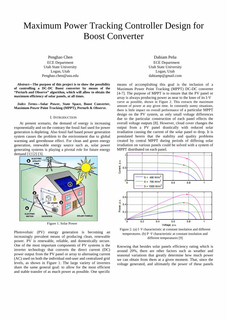
I. INTRODUCTION At present scenario, the demand of energy is increasing

exponentially and on the contrary the fossil fuel used for power generation is depleting. Also fossil fuel based power generation system causes the problem to the environment due to global warming and greenhouse effect. For clean and green energy generation, renewable energy source such as, solar power generating systems is playing a pivotal role for future energy demand [1] [2] [3].

Figure 1. Solar Power

Photovoltaic (PV) energy generation is becoming an increasingly prevalent means of producing clean, renewable power. PV is renewable, reliable, and domestically secure. One of the most important components of PV systems is the inverter technology that converts the direct current (DC) power output from the PV panel or array to alternating current (AC) used on both the individual end-user and centralized grid levels, as shown in Figure 1. The large variety of inverters share the same general goal: to allow for the most efficient and stable transfer of as much power as possible. One specific

means of accomplishing this goal is the inclusion of a Maximum Power Point Tracking (MPPT) DC-DC converter [4-7]. The purpose of MPPT is to ensure that the PV panel or array is always producing power as near to the knee of its I-V curve as possible, shown in Figure 2. This extracts the maximum amount of power at any given time. In constantly sunny situations, there is little impact on overall performance of a particular MPPT design on the PV system, as only small voltage differences due to the particular construction of each panel effects the overall voltage outputs [8]. However, cloud cover changes the output from a PV panel drastically with reduced solar irradiation causing the current of the solar panel to drop. It is postulated herein that the stability and quality problems created by central MPPT during periods of differing solar irradiation on various panels could be solved with a system of MPPT distributed on each panel.

Figure 2. (a) I–V characteristic at constant insolation and different

temperatures. (b) P–V characteristic at constant insolation and different temperatures [9]

Knowing that besides solar panels efficiency rating which is around 20%, there are other factors such as weather and seasonal variations that greatly determine how much power we can obtain from them at a given moment. That, since the voltage generated, and ultimately the power of these panels

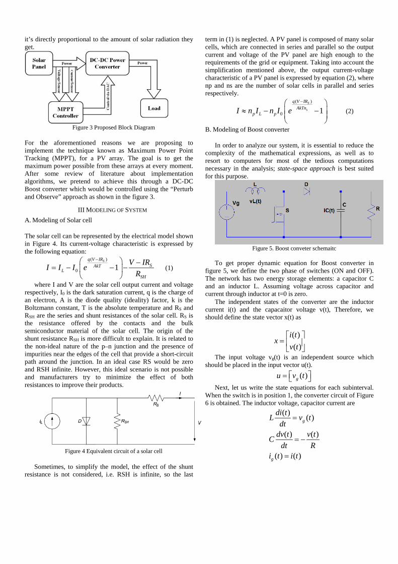
it’s directly proportional to the amount of solar radiation they get.

Figure 3 Proposed Block Diagram

For the aforementioned reasons we are proposing to implement the technique known as Maximum Power Point Tracking (MPPT), for a PV array. The goal is to get the maximum power possible from these arrays at every moment. After some review of literature about implementation algorithms, we pretend to achieve this through a DC-DC Boost converter which would be controlled using the “Perturb and Observe” approach as shown in the figure 3.

III MODELING OF SYSTEM A. Modeling of Solar cell

The solar cell can be represented by the electrical model shown in Figure 4. Its current-voltage characteristic is expressed by the following equation:

( )

0 1Sq V IR

SAkTL

SH

V IRI I I eR

− −= − − −

(1)

where I and V are the solar cell output current and voltage respectively, I0 is the dark saturation current, q is the charge of an electron, A is the diode quality (ideality) factor, k is the Boltzmann constant, T is the absolute temperature and RS and RSH are the series and shunt resistances of the solar cell. RS is the resistance offered by the contacts and the bulk semiconductor material of the solar cell. The origin of the shunt resistance RSH is more difficult to explain. It is related to the non-ideal nature of the p–n junction and the presence of impurities near the edges of the cell that provide a short-circuit path around the junction. In an ideal case RS would be zero and RSH infinite. However, this ideal scenario is not possible and manufacturers try to minimize the effect of both resistances to improve their products.

Figure 4 Equivalent circuit of a solar cell

Sometimes, to simplify the model, the effect of the shunt

resistance is not considered, i.e. RSH is infinite, so the last

term in (1) is neglected. A PV panel is composed of many solar cells, which are connected in series and parallel so the output current and voltage of the PV panel are high enough to the requirements of the grid or equipment. Taking into account the simplification mentioned above, the output current-voltage characteristic of a PV panel is expressed by equation (2), where np and ns are the number of solar cells in parallel and series respectively.

( )

0 1S

s

q V IRAkTn

p L pI n I n I e−

≈ − −

(2)

B. Modeling of Boost converter In order to analyze our system, it is essential to reduce the

complexity of the mathematical expressions, as well as to resort to computers for most of the tedious computations necessary in the analysis; state-space approach is best suited for this purpose.

Figure 5. Boost conveter schemaitc

To get proper dynamic equation for Boost converter in

figure 5, we define the two phase of switches (ON and OFF). The network has two energy storage elements: a capacitor C and an inductor L. Assuming voltage across capacitor and current through inductor at t=0 is zero.

The independent states of the converter are the inductor current i(t) and the capacaitor voltage v(t), Therefore, we should define the state vector x(t) as

( )( )

i tx

v t

=

The input voltage vg(t) is an independent source which should be placed in the input vector u(t).

( )gu v t =

Next, let us write the state equations for each subinterval. When the switch is in position 1, the converter circuit of Figure 6 is obtained. The inductor voltage, capacitor current are

( ) ( )

( ) ( )

( ) ( )

g

g

di tL v tdt

dv t v tCdt R

i t i t

=

= −

=

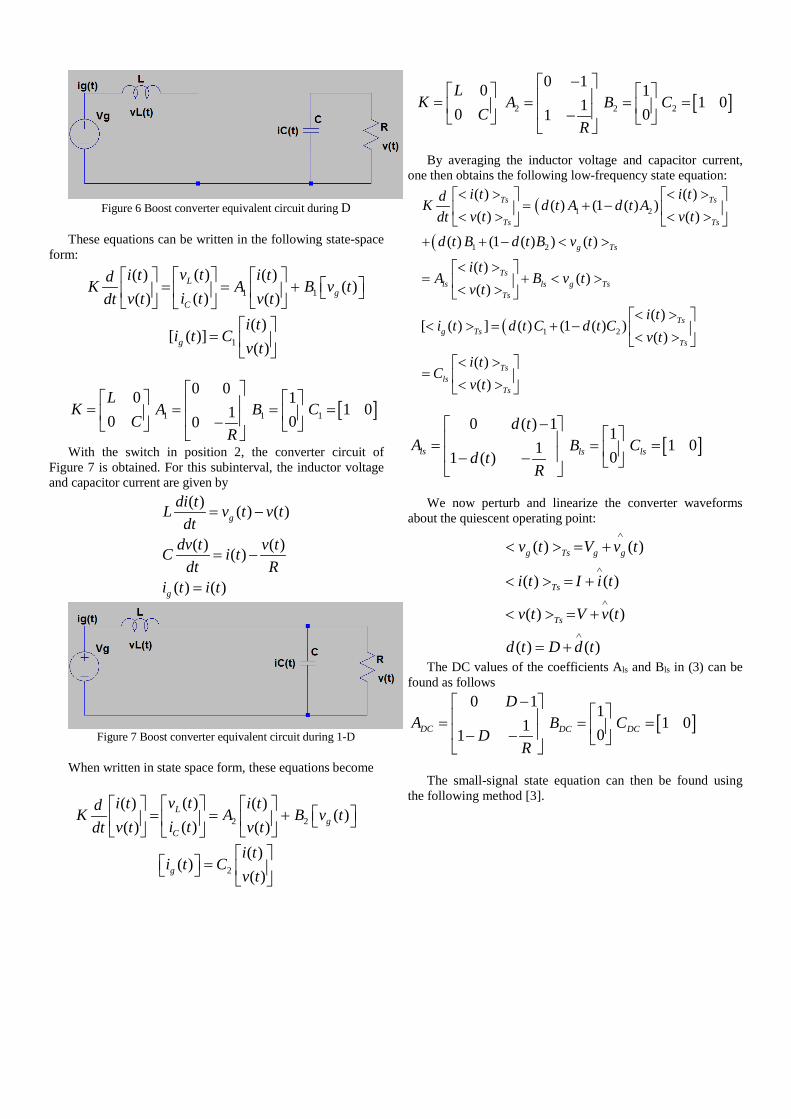
Figure 6 Boost converter equivalent circuit during D

These equations can be written in the following state-space

form:

1 1

( )( ) ( )( )

( )( ) ( )L

gC

v ti t i tdK A B v ti tv t v tdt

= = +

1

( )[ ( )]

( )g

i ti t C

v t

=

00L

KC

=

1

0 010

AR

= −

1

10

B =

[ ]1 1 0C =

With the switch in position 2, the converter circuit of Figure 7 is obtained. For this subinterval, the inductor voltage and capacitor current are given by

( ) ( ) ( )

( ) ( )( )

( ) ( )

g

g

di tL v t v tdt

dv t v tC i tdt R

i t i t

= −

= −

=

Figure 7 Boost converter equivalent circuit during 1-D

When written in state space form, these equations become

2 2

( )( ) ( )( )

( )( ) ( )L

gC

v ti t i tdK A B v ti tv t v tdt

= = +

2

( )( )

( )g

i ti t C

v t

=

00L

KC

=

2

0 111

AR

− = −

2

10

B =

[ ]2 1 0C =

By averaging the inductor voltage and capacitor current,

one then obtains the following low-frequency state equation:

(

(

(

1 2

1 2

1 2

( ) ( )( ) (1 ( ) )

( ) ( )

( ) (1 ( ) ) ( )

( )( )

( )

( )[ ( ) ] ( ) (1 ( ) )

( )

( )( )

Ts Ts

Ts Ts

g Ts

Tsls ls g Ts

Ts

Tsg Ts

Ts

Tsls

i t i tdK d t A d t Av t v tdt

d t B d t B v t

i tA B v t

v t

i ti t d t C d t C

v t

i tC

v t

< > < > = + − < > < >

+ + − < >

< > = + < > < >

< > < > = + − < >

< >=

< Ts

>

0 ( ) 1

11 ( )ls

d tA

d tR

− = − −

10lsB

=

[ ]1 0lsC =

We now perturb and linearize the converter waveforms

about the quiescent operating point:

( ) ( )g Ts g gv t V v t∧

< > = +

( ) ( )Tsi t I i t∧

< > = +

( ) ( )Tsv t V v t∧

< > = +

( ) ( )d t D d t∧

= + The DC values of the coefficients Als and Bls in (3) can be

found as follows 0 1

11DC

DA

DR

− = − −

10DCB

=

[ ]1 0DCC =

The small-signal state equation can then be found using

the following method [3].

1 2 1 2

1 2

( ) ( )( )

( ) ( )

( ) ( ) ( )

( )[ ( )] ( ) ( )

( )

DC DC g

g

g DC

i t i tdK A B v tv tdt v t

IA A B B V d t

V

i t Ii t C C C d t

Vv t

∧∧

∧

∧

∧∧

∧

= + +

− + − = + −

After simplification, we get the following:

( ) ( ) ( )( ) ( ) ( )

( )[ ( )]

( )

gss ss

g ss

i t i t v td A Bv tdt v t d t

i ti t C

v t

∧ ∧

∧ ∧

∧

∧

= + =

10

1 1ss

DLA

DC CR

−

= − −

1

0ss

VL LB

IC

= −

[ ]1 0ssC = Equation (4) is the linearized small-signal state equation of the boost converter. Ass and Bss contain only AC terms. The stability of this matrix can be determined by the following analysis [4]. The stability of the boost converter can be determined by checking the eigenvalues λ:

22 1 (1 )det( ) 0DA I

RL LCλ λ λ −

− = + + =

So, 2

21 1 1 4(1 )( )2

DRL RL LC

λ − −

= ± −

The DC operating parameter listed in the Table I. Because all the parameter value are positive, the eigenvalue of the boost converter are negative. Thus, the boost converter system is asymptotically stable. By checking the rank of the controllability matrix

[ ]B AB and oberverability matrixC

CA

, their ranks are

equal to n. So the boost converter system is either controllable or observable.

III SIMULINK MODEL OF BOOST CONVERTER A. Solar Panel Simulink Model

The solar panel is consist of 72 solar cells in series shown

in the figure 8. The model built using the sim Power system symbol blocks in the Matlab library. The open circuit voltage and short current of solar cell is 0.6V and 4.75A, respectively.

Figure 8. The Simulink model of solar panel.

B. Boost Converter Simulink Model The Simulink model of Boost converter is shown in the

figure 9. In order to validate the function of Boost converter, the ideal switch and diode is implemented in the Simulink model, and the DC operating parameter value is shown in the table I.

Table I DC operating parameter Parameter Value Unit

C 47 uF L 1.5 mH R 16 Ω

Frequency 50 kHz

Figure 9. The Simulink model of Boost covnerter

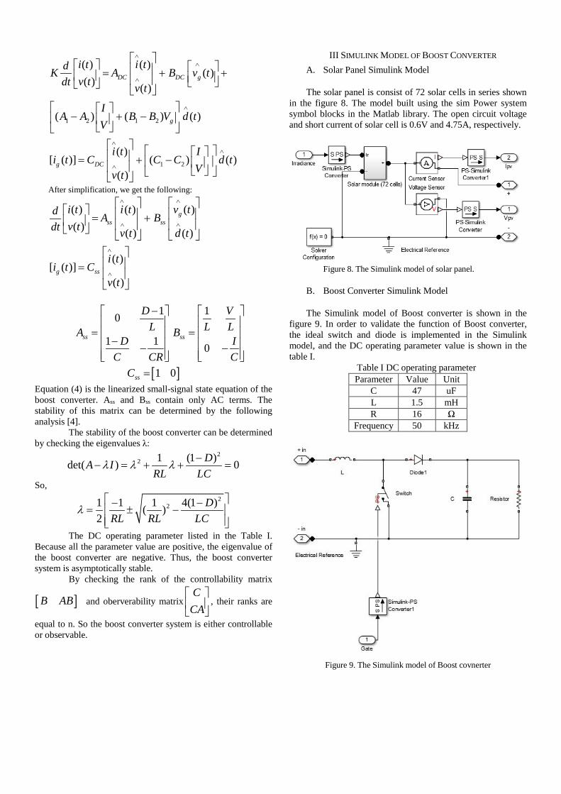
C. MPPT Algorithm

The P&O algorithm is also called “hill-climbing”, but both

names refer to the same algorithm. Hill-climbing involves a perturbation on the duty cycle of the power converter and P&O a perturbation in the operating voltage of the DC link between the PV array and the power converter. In the case of the Hill-climbing, perturbing the duty cycle of the power converter implies modifying the voltage of the DC link between the PV array and the power converter, so both names refer to the same technique.

In this method, the sign of the last perturbation and the sign of the last increment in the power are used to decide what the next perturbation should be. As can be seen in Figure 11, on the left of the MPP incrementing the voltage increases the power whereas on the right decrementing the voltage increases the power.

Figure 10 power profile of solar cell.

If there is an increment in the power, the perturbation

should be kept in the same direction and if the power decreases, then the next perturbation should be in the opposite direction. Based on these facts, the algorithm is implemented in the figure 11. The process is repeated until the MPP is reached.

Start

Read V(k),I(k) from Array

P(k)=V(k)*I(k)

ΔP=P(k)-P(k-1)ΔV=V(k)-V(k-1)

ΔP>0

ΔV>0 ΔV>0

D(k)=D(k-1)+ΔD D(k)=D(k-1)-ΔD D(k)=D(k-1)-ΔD D(k)=D(k-1)+ΔD

Yes No

Return

Yes YesNo No

Figure 11 Flowchart of P&O algorithm

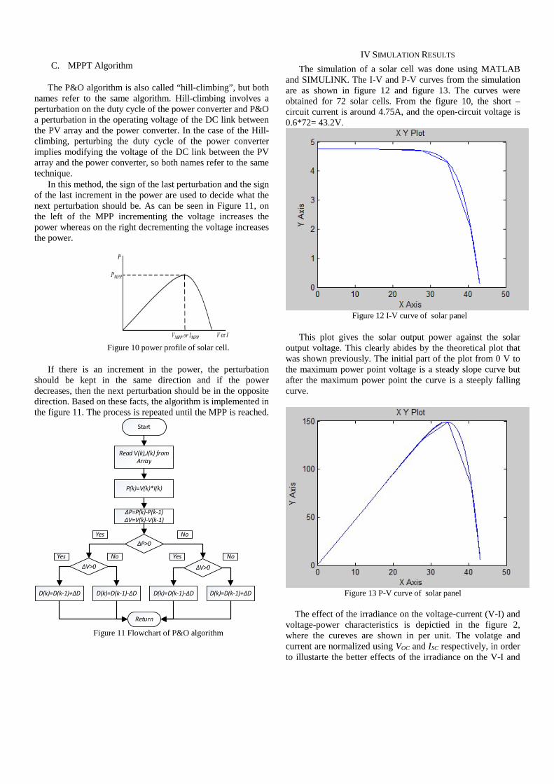
IV SIMULATION RESULTS The simulation of a solar cell was done using MATLAB

and SIMULINK. The I-V and P-V curves from the simulation are as shown in figure 12 and figure 13. The curves were obtained for 72 solar cells. From the figure 10, the short –circuit current is around 4.75A, and the open-circuit voltage is 0.6*72= 43.2V.

Figure 12 I-V curve of solar panel

This plot gives the solar output power against the solar

output voltage. This clearly abides by the theoretical plot that was shown previously. The initial part of the plot from 0 V to the maximum power point voltage is a steady slope curve but after the maximum power point the curve is a steeply falling curve.

Figure 13 P-V curve of solar panel

The effect of the irradiance on the voltage-current (V-I) and voltage-power characteristics is depictied in the figure 2, where the cureves are shown in per unit. The volatge and current are normalized using VOC and ISC respectively, in order to illustarte the better effects of the irradiance on the V-I and

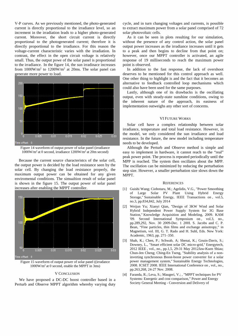
V-P curves. As we previously mentioned, the photo-generated current is directly proportional to the irradiance level, so an increment in the irradiation leads to a higher photo-generated current. Moreover, the short circuit current is directly proportional to the photogenerated current; therefore it is directly proportional to the irradiance. For this reason the voltage-current characteristic varies with the irradiation. In contrast, the effect in the open circuit voltage is relatively small. Thus, the output powe of the solar panel is proportional to the irradiance. In the figure 14, the sun irradinace increases from 1000W/m2 to 1200W/m2 at 20ms. The solar panel can generate more power to load.

Figure 14 waveform of output power of solar panel (irradiance 1000W/m2 at 0 second, irradiance 1200W/m2 at 20m second)

Because the current source characteristcs of the solar cell, the output power is decided by the load resistance seen by the solar cell. By changing the load resistance properly, the maximum output power can be obtained for any given enviromental conditions. The simualtion result of solar panel is shown in the figure 15. The output power of solar panel increases after enabling the MPPT controller.

Figure 15 waveform of output power of solar panel ((irradance

1000W/m2 at 0 secend, enable the MPPT in 3ms)

V CONCLUSION We have proposed a DC-DC boost controller based in a

Perturb and Observe MPPT algorithm whereby varying duty

cycle, and in turn changing voltages and currents, is possible to extract maximum power from a solar panel comprised of 72 solar photovoltaic cells.

As it can be seen in plots resulting for our simulation, without the presence of any control action, the solar panel output power increases as the irradiance increases until it gets to a peak and then begins to decline from that point on; however, once our MPPT controller is activated, an agile response of 19 milliseconds to reach the maximum power point is observed.

In addition to the fast response, the lack of overshoot deserves to be mentioned for this control approach as well. One other thing to highlight is and the fact that it becomes an alternative to feedback controlled loop mechanisms which could also have been used for the same purposes.

Lastly, although one of its drawbacks is the oscillating output, even with steady-state sunshine conditions, owing to the inherent nature of the approach, its easiness of implementation outweighs any other sort of concerns.

VI FUTURE WORKS Solar cell have a complex relationship between solar

irradiance, temperature and total load resistance. However, in the model, we only considered the sun irradiance and load resistance. In the future, the new model including temperature needs to be developed.

Although the Perturb and Observe method is simple and easy to implement in hardware, it cannot reach to the “real” peak power point. The process is repeated periodically until the MPP is reached. The system then oscillates about the MPP. The oscillation can be minimized by reducing the perturbation step size. However, a smaller perturbation size slows down the MPPT.

REFERENCES [1] Guishi Wang; Ciobotaru, M.; Agelidis, V.G., "Power Smoothing

of Large Solar PV Plant Using Hybrid Energy Storage," Sustainable Energy, IEEE Transactions on , vol.5, no.3, pp.834,842, July 2014

[2] Weijun Yu; Xianyi Qian, "Design of 3KW Wind and Solar Hybrid Independent Power Supply System for 3G Base Station," Knowledge Acquisition and Modeling, 2009. KAM '09. Second International Symposium on , vol.3, no., pp.289,292, Nov. 30 2009-Dec. 1 200I. S. Jacobs and C. P. Bean, “Fine particles, thin films and exchange anisotropy,” in Magnetism, vol. III, G. T. Rado and H. Suhl, Eds. New York: Academic, 1963, pp. 271–350.

[3] Shah, K.; Chen, P.; Schwab, A; Shenai, K.; Gouin-Davis, S.; Downey, L., "Smart efficient solar DC micro-grid," Energytech, 2012 IEEE , vol., no., pp.1,5, 29-31 May 2012Jaw-Kuen Shiau; Chun-Jen Cheng; Ching-En Tseng, "Stability analysis of a non-inverting synchronous Boost-boost power converter for a solar power management system," Sustainable Energy Technologies, 2008. ICSET 2008. IEEE International Conference on , vol., no., pp.263,268, 24-27 Nov. 2008.

[4] Faranda, R.; Leva, S.; Maugeri, V.; , ”MPPT techniques for PV Systems: Energetic and cost comparison,” Power and Energy Society General Meeting - Conversion and Delivery of

Electrical Energy in the 21st Century, 2008 IEEE , vol., no., pp.1-6, 20-24 July 2008

[5] Lopez-Lapena, O.; Penella, M.T.; Gasulla, M., "A New MPPT Method for Low-Power Solar Energy Harvesting," Industrial Electronics, IEEE Transactions on , vol.57, no.9, pp.3129,3138, Sept. 2010)

[6] Guan-Chyun Hsieh; Hung-I Hsieh; Cheng-Yuan Tsai; Chi-Hao Wang, "Photovoltaic Power-Increment-Aided Incremental-

[7] Conductance MPPT With Two-Phased Tracking," Power Electronics, IEEE Transactions on , vol.28, no.6, pp.2895,2911, June 2013

[8] Barchowsky, A; Parvin, J.P.; Reed, G.F.; Korytowski, M.J.; Grainger, B.M., "A comparative study of MPPT methods for distributed photovoltaic generation," Innovative Smart Grid Technologies (ISGT), 2012 IEEE PES , vol., no., pp.1,7, 16-20 Jan. 2012

[9] P. Bhatnagar and R. Nema, “Maximum power point tracking control techniques: State-of-the-art in photovoltaic applications,” Renewable and Sustainable Energy Reviews, vol. 23, no. 0, pp. 224 – 241, 2013