Modeling Category Viewership of Web Users with Multivariate Count

Print Date: 7/15/2002

Modeling Category Viewership of Web Users with Multivariate Count Models

Shibo Li, John C. Liechty, and Alan L. Montgomery

July 2002

Shibo Li ([email protected]) is a Ph.D. Candidate and Alan L. Montgomery (e-mail: [email protected]) is an Associate Professor at the Graduate School of Industrial Administration, Carnegie Mellon University, 5000 Forbes Ave., Pittsburgh, PA 15213. John C. Liechty ([email protected]) is an Assistant Professor of Marketing and Statistics at the Pennsylvania State University, 710 M Business Administration Building, University Park, PA 16802. The corresponding author is Alan L. Montgomery. The authors wish to thank Jupiter Media Metrix for their generous contribution of data without which this research would not have been possible.

Copyright © 2002 by Shibo Li, John C. Liechty, and Alan L. Montgomery, All rights reserved

1

Modeling Category Viewership of Web Users

with Multivariate Count Models

Abstract:

We develop a statistical model of browsing behavior by predicting the number of web pages, in a

particular category, that are viewed by a user in a single web session. The purpose of this analysis is

to better understand web browsing behavior, and to help predict which sessions are likely to result in

retail visits. A single record in our database consists of the number of web pages viewed by a user

during a single session from each of the following categories: portals, services, entertainment, retail,

auctions, adult, and others. This dataset can be characterized as multivariate count data, where many

of the counts are zero. We consider the use of Poisson and discretized tobit models, and contrast

both univariate and multivariate versions of these models. Additionally, as our dataset is

characterized by a great deal of heterogeneity in usage across users and also a good deal of

persistence in viewership, we propose a new multivariate tobit model with a mixture process whose

multiple states are governed by an unobserved (hidden) Markov chain. We find that users move

between sessions that are characterized by browsing behavior that is focused in specific categories

and sessions characterized by a variety of categories being viewed.

Keywords: Multivariate Count Data, Internet Usage, Tobit Models, Hierarchical Bayes

Models, Hidden Markov Chain Models, Markov Switching Models

2

1. Introduction In this study we consider the category of web viewings made by a user during a session.

Consumer web browsing behavior is quite diverse both in terms of the type of information that can

be viewed and the diversity of the user base. For example, a businessman going on a trip may visit a

portal and search for information about a conference, buy an airline ticket, and reserve a hotel room.

A student using a laptop with a wireless connection search for their favorite music, download music

files, and bid at an Ebay auction—all while listening to their professor lecture. In our example, the

businessman visited a portal and two retail sites, while the student visited a portal, retail, and auction

site. Our goal is to describe the joint distribution of the number of web pages from different

categories that were viewed during a web session. In particular, we are interested in reviewing the

properties of a range of univariate and multivariate statistical models that could be used to model this

data and in exploring the insights into web browsing behavior that can be gained from these models.

Understanding category viewership of web users is of interest to web designers, marketing

researchers, and cognitive psychologists, as well as many others. Web designers need to understand

how consumers use web sites in order to improve their site designs (Nielsen 2000). For example, do

consumers tend to focus upon only one topic during a session (e.g., shopping) or do they view

several (e.g., auctions, entertainment, and shopping)? Marketing researchers want to predict which

web sessions are likely to result in shopping behavior, so they can focus their advertising efforts on

these occasions (Gooley and Lattin 2001). Cognitive psychologists are interested in determining

whether consumers are foraging for information or simply gathering it (Pirolli and Card 1999).

Information foraging makes an analogy between the strategies users have for locating information

(e.g., surfing the web) and the evolutionary economical explanations for food-foraging strategies

from anthropology and behavioral ecology.

We develop a statistical model of browsing behavior which predicts the number of web

pages viewed by a user during a single web session in seven categories: portals, services,

entertainment, retail, auctions, adult and other. A single record in our database consists of the

number of viewings by a user during a single session in the each of these categories. For example, a

user starts a session at google.com and visits three pages in the course of a search for a book, locates a

book description at an entertainment site, and follows up with a one-click purchase of the book at

amazon.com. The resulting dataset from this visit would be: portal (3), entertainment (1), retail (2), and

zero for the remaining categories. Our dataset can be characterized as multivariate counts.

3

There is an extensive literature on modeling count data. We refer the reader to Cameron

and Trivedi (1986) and Patil (1970) for a more extensive review and survey of the literature and to

Atchison and Ho (1989) for a discussion of multivariate Poisson Log normal models of multivariate

count data. Some selected applications of count models include children’s spelling errors (van Duijn

and Böckenholt, 1995), technological innovation (Blundell, Griffith, and Reenen, 1995), purchases

for a frequently bought consumer goods (Ramaswamy, Anderson, and Desarbo, 1994), consumer

purchases of books offered through direct mail (Wedel, et. al., 1993), unemployment spells (Brännäs,

1992), recreational fishing trips (Grogger and Carson, 1991), premature ventricular contractions

(Farewell and Sprott, 1988).

Statistically there are several interesting aspects to our dataset that contrasts with previous

work. First, our data is made up of multivariate counts, where the counts are often zero. As this

censoring can mask multivariate relationships, we contrast univariate and multivariate versions of

count models to illustrate these differences. Second, our dataset is characterized by a great deal of

heterogeneity in usage across users. We introduce a hierarchical Bayesian model to accommodate

this heterogeneity. Third, there is a time series element to browsing behavior. We find that users

exhibit a good deal of persistence in their browsing, that is they tend to have sessions that are either

focused upon viewings in specific categories or ones that view a large variety of categories. To

capture all these elements we develop a new, discretized version of a multivariate tobit model with a

mixture process whose multiple states are governed by an unobserved (hidden) Markov chain. To

motivate the construction of this model we present a series of count models that progressively add

each of these elements. Our pedagogical approach is to illustrate the deficiencies of simpler models

and show how our proposed framework can overcome these weaknesses.

The study of statistical properties of web browsing behavior has a brief history. Huberman

et al (1998) found that the distribution of the number of web pages visited has a long tail and can be

approximated fairly well with an inverse Gaussian distribution. Bucklin and Sismeiro (2001) use

information from the timing between page views to predict whether users will continue browsing.

Cadez et al (2000) and Deshpande and Karypis (2000) employ Markov Models to study browsing

patterns. Moe and Fader (2001) study repeat visit behavior and purchase conversion rates at

Amazon and CDNow. These studies focus primarily on browsing behavior within a web site. Other

research focuses on browsing behavior across web sites. Montgomery and Faloutos (2002) found

that many measures of browsing behavior are stable through time. Johnson et al. (2002) study

product search behavior and found that web browsers are engaging in only a limited amount of

4

searches across web sites for products. For example, the average number of stores visited by book

buyers in 1998 was 1.1. Our study contributes to this growing literature by describing usage behavior

and presenting a compatible model for its study. It also helps bridge the gap between past research

by examining session level behavior as opposed to page-by-page level analyses and aggregate level

usage studies where the browsing behavior is aggregated at a monthly level.

The outline of our paper is as follows. In section 2 we define and describe our dataset and

problem. We describe various statistical approaches for modeling count data in section 3, starting

with univariate approaches and generalizing to multivariate ones in section 4. We discuss our results

in section 4, and motivate the construction of a new model to deal with the observed discrepancies

between our data and standard models of count data. Section 5 concludes the paper with a summary

and discussion of our findings.

Category Domain Reach (%)Auction Ebay.com

Ubid.com Auctionwatch.com

23.1 16.3 2.8

Entertainment Real.com Snap.com About.com

17.5 12.5 12.1

Portals Yahoo.com MSN.com AOL.com

62.7 52.2 44.6

Retailing Amazon.com Americangreetings.com Webstakes.com

18.8 10.0 6.9

Service Microsoft.com Passport.com Hotmail.com

39.3 29.0 26.9

Table 1. Listing of most frequently visited domains in each category.

2. Data Our data is derived from a panel of web users constructed by Jupiter Media Metrix (JMM).

JMM randomly recruits a representative sample of personal computers users and tracks their usage at

home and/or work (Coffey 1999). These panelists agree to run a program that runs in the

background on their computer and monitors computer usage. It records any URL viewed by the

user in their browser window. Since it records the actual pages viewed at the source, it avoids

caching problems commonly found by recording page requests at their Internet Service Provider

(ISP) or a web server. Each page viewing, or more precisely the domain of the page viewing, is

5

classified by JMM into one of seven categories: portals, services, entertainment, retail, auctions, adult

and other. Examples of the top three domains in each of these categories are listed in Table 1 along

with the percentage of individuals who visited the domain at least once during the month (Reach) for

July 2000. For example, Amazon is the most popular retail site and was visited by 18.8% of users.

We should note that these domains represent only a small fraction of the web sites in each category.

Number of Page Views in Each Category Sess-ion Start Time Auction

Enter-tainment Portals Retail Service Adult Others

1 04Oct2000: 17:32:54 0 0 0 0 0 0 55 2 06Oct2000: 00:58:47 0 0 0 0 8 0 7 3 09Oct2000: 14:09:42 0 0 4 0 8 0 50 4 10Oct2000: 17:28:23 0 0 0 0 8 0 9 5 11Oct2000: 10:50:38 0 0 0 0 6 0 9 6 11Oct2000: 17:18:18 0 0 0 0 5 0 1 7 16Oct2000: 14:38:32 0 0 0 10 7 0 1 8 19Oct2000: 22:58:45 0 0 0 0 10 0 14 9 20Oct2000: 23:10:33 0 0 30 0 7 0 59 10 23Oct2000: 14:07:07 0 0 0 0 10 0 1 11 28Oct2000: 12:06:59 0 0 16 0 0 0 21 12 29Oct2000: 10:16:34 0 0 0 0 0 0 2 13 29Oct2000: 19:33:41 0 0 2 26 28 0 9 14 02Nov2000: 14:05:36 0 0 0 3 4 0 19 15 05Nov2000: 12:20:58 0 0 2 0 5 0 2 16 05Nov2000: 22:04:06 0 0 7 0 4 0 2 17 07Nov2000: 22:30:58 0 0 0 51 56 0 71 18 09Nov2000: 11:26:28 0 0 1 0 15 0 6 19 09Nov2000: 23:47:26 0 0 0 0 5 0 1 20 26Nov2000: 17:11:54 0 0 0 0 7 0 52

Table 2. Data for a selected panelist (white, male, age 23).

Our dataset consists of the browsing behavior of 300 randomly selected users and was

collected between July 1997 and November 2000. The average user has an average of 441 sessions,

which yields a total of 132,368 sessions. The mean age of our users is 52 years old (standard

deviation of 17), with a minimum or 7 and maximum of 84. Also, 68% of users are male and 83%

are white. To illustrate, the usage information for one individual is listed in Table 2 for twenty out of

a total of 140 sessions. A session is defined as period of sustained web browsing, and ends after

twenty minutes of inactivity. There are several characteristics that we would like to point out that are

illustrated by this example. First notice the user never visits three of the categories: auction,

entertainment, and adult. Also, some sessions can be characterized by their extensive use in a

particular category like shopping or its absence. Second, the number of viewings in a category tends

6

to have a distribution with a long tail. Finally, it is likely that usage in one category may be related to

usage in another category (e.g., searches at portals should lead to more viewings).

We also list the descriptive statistics of the number of page viewings in each category across

our 300 users in Table 3. Notice that portals are the most commonly viewed pages, and account for

15.8% of all viewings, followed by adult and service. The most frequently visited category in our

scheme is Other, which accounts for 36.5% of usage. To measure the relationship between categories

we compute the sample correlations in Table 4. A cursory examination of these correlations shows

only weak relationships, with an average correlation of 0.067, and the largest correlation being .21

between the portal and other category. This may lead one to conclude that there is little relationship

amongst these categories, but as we will show in our subsequent analyses this is a premature

conclusion.

No. of viewings given that at least one viewed

Percentiles

Category Mean Std. Dev. 25th Median 75th Max

Probability of no viewings during session Mean Variance

Auction 25.16 46.79 2 8 28 710 0.93 1.72 190.44 Entertainment 16.11 46.56 2 5 14 1848 0.82 2.86 422.30 Portals 11.03 29.06 2 4 11 2005 0.57 4.70 389.66 Retailing 12.09 28.23 2 5 13 2501 0.86 1.65 126.34 Service 12.98 25.55 2 5 14 1314 0.70 3.94 233.78 Adult 40.17 78.25 2 10 41 1415 0.90 4.07 767.29 Others 15.49 27.28 3 7 17 1008 0.30 10.89 573.12

Table 3. Descriptive statistics of the number of page viewings in each category based upon a sample of 132,368 sessions.

Auction

Enter-tainment Portals Retailing Service Adult Others

Auction 1 Entertainment 0.027 1 Portals 0.014 0.034 1 Retailing 0.041 0.052 0.021 1 Service 0.025 0.123 0.054 0.047 1 Adult 0.023 -0.008 0.118 0.008 0.065 1 Others 0.019 0.044 0.210 0.045 0.084 0.117 1

Table 4. Sample Correlation of the Number of Page Viewing across Categories based upon a sample of 132,368 sessions.

7

0 5 0 1 0 0 1 5 0 2 0 0 2 5 0

020

000

4000

060

000

8000

010

0000

1200

00

R e ta i l V ie w in g s P e r S e s s io n

Freq

uenc

y

Figure 1. Histogram of Number of Viewings Per Session in the Retail Category.

0 5 0 1 0 0 1 5 0 2 0 0 2 5 0

100

101

102

103

104

105

R e t a i l V ie w in g s P e r S e s s io n

Freq

uenc

y

Figure 2. Histogram of Number of Viewings Per Session in the Retail Category on a Log Scale, Zero Excluded.

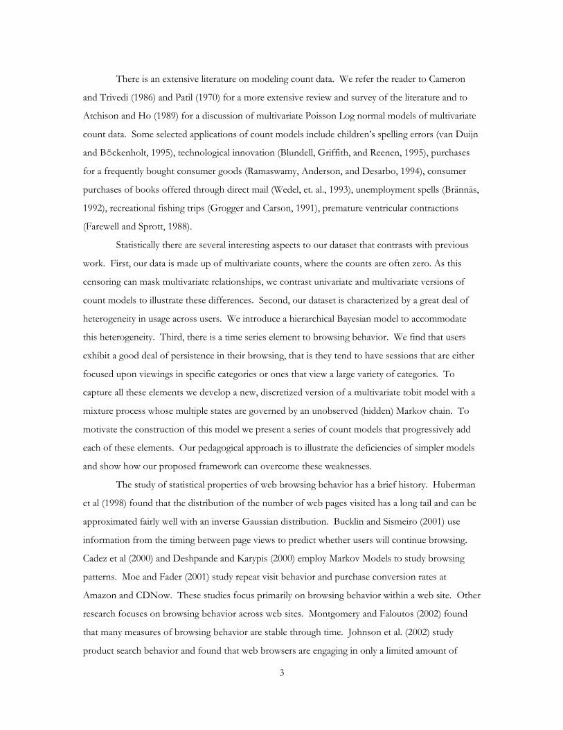
3. Modeling Category Viewing with Univariate Models To motivate our modeling discussion, we summarize our data by plotting the histogram of

the number of web pages viewed during a session from the retail category; see Figure 1. (We omit

one outlier with 2501 viewings from this and subsequent figures.) The huge spike at zero (86% of

viewings as reported in Table 3) and a very long tail makes the natural scale quite compressed, so we

plot the histogram again in Figure 2 using a log scale for the y-axis. Our first problem is to introduce

a model that is able to capture the type of marginal distribution exhibited in Figure 2. In addition to

8

the large number of sessions with zero viewings and the variety in the number of viewings for the

remaining sessions, there are several aspects of our data that are important to capture: discrete,

multivariate, heterogeneity across users, and time series behavior. In the next section we will propose

a model that incorporates all of these aspects. To motivate this model we define a series of models

that become progressively more complicated models as they incorporate selected elements of the full

model. Our purpose in following this approach is to better understand the contribution of each of

these elements and their potential weakness.

We begin with the standard Poisson regression model in section 3.1. Next we introduce a

univariate tobit model and contrast the results with the Poisson model. We suggest two

modifications to the tobit model to improve over the Poisson model, namely an exponential

transformation and discretization. Next we show our tobit model can be placed in the context of a

hierarchical Bayesian framework to capture individual level heterogeneity. We find that this model is

a good approximation to the marginal behavior of the underlying phenomena. In Section 4 we

extend the modeling framework from univariate to multivariate, by considering a multivariate tobit

model, and finally we introduce a version of the multivariate tobit model that allows time-varying

browsing behavior.

3.1. Univariate Poisson Model Perhaps the most popular model of count processes, due to its simplicity, is the Poisson

regression model. In our problem we have a large spike at zero and introduce a truncated model

with a mixture process at 0 to account for the large number of zero values:

c

c

p-1y probabilit with )(

py probabilit with 0~

ictict ZPoisson

Z (1)

icict XZ ')ln( γ= (2)

Where ictZ is user i’s number of viewings in domain category c in session t (i = 1, …, I; c = 1, …, C; t

= 1, …, Ti). ictZ is the mean of ictZ . iX is an L × 1 vector that consists of covariates such as

demographic variables. In our empirical application, iX includes user i’s age (with log

transformation), gender and race (whether the user is white or not). icγ is an L × 1 vector of

coefficients. The expectation and variance of ictZ in (1) conditional upon iX is:

ic Xictiict epZpXZE ')1()1()|( γ−=⋅−= (3)

Standard maximum likelihood estimation (MLE) techniques are used to estimate the

parameters in the model using SAS software. The MLE estimates of the p parameters are the same

9

as the probability of no viewings during a session as reported in Table 3 (e.g., the estimate for p in the

retail category is 0.86), and the remaining parameter estimates are given in table 5. Notice that all of

the parameter estimates appear to be highly statistically significant. Notably we find that age

decreases the expected viewings per category, while gender and race have mixed effects. Men tend to

view portals and adult sites with greater frequency than women, and white individuals are more likely

to view auction, portals, service, and adult.

Dependent Variable Intercept Log(Age) Gender White

Expected Mean

Auction 5.29 (0.029)

-0.65 (0.007)

-0.05 (0.004)

0.42 (0.007)

1.57 (0.48)

Entertainment 4.78 (0.015)

-0.46 (0.004)

-0.12 (0.004)

-0.29 (0.004)

2.66 (0.67)

Portals 3.39 (0.013)

-0.35 (0.003)

0.22 (0.003)

0.12 (0.004)

4.27 (0.69)

Retailing 4.25 (0.024)

-0.48 (0.006)

-0.01 (0.005)

-0.02 (0.006)

1.52 (0.29)

Service 4.28 (0.014)

-0.48 (0.003)

-0.27 (0.003)

0.23 (0.004)

3.47 (0.89)

Adult 2.67 (0.015)

-0.14 (0.004)

1.11 (0.007)

0.55 (0.006)

3.28 (1.45)

Others 3.99 (0.009)

-0.34 (0.002)

-0.08 (0.002)

0.09 (0.002)

10.27 (1.51)

Table 5. Estimation Results for Poisson Models. The standard errors are given in parenthesis below the estimate.

The mean, which is the same as the variance in the Poisson model, and their standard errors

are included in the final column. For example, the expected value of retailing in our panel is 1.5

viewings per session. To illustrate the distribution of these predictions we overlay the predicted

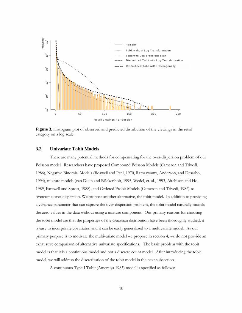
marginal distribution against the realized data in Figure 3. A major deficiency of the Poisson model,

as commonly happens in practice, is the problem of over-dispersion. Most of the mass of the

Poisson models is over small values (between 0 and 8 viewings per session). However, the data has a

long tail that the Poisson model is not able to capture since it has only a single parameter to capture

both the mean and variance.

10

0 50 100 150 200 250

100

101

102

103

104

105

R e ta il V iew ings P er S ess ion

Freq

uenc

yP o isson

T ob it w ith ou t Log T ra ns fo rm ation

T ob it w ith Log T rans fo rm ation

D isc re tized T ob it w ith Log T rans fo rm ation

D isc re tize d T ob it w ith H e te rogen e ity

Figure 3. Histogram plot of observed and predicted distribution of the viewings in the retail category on a log scale.

3.2. Univariate Tobit Models There are many potential methods for compensating for the over-dispersion problem of our

Poisson model. Researchers have proposed Compound Poisson Models (Cameron and Trivedi,

1986), Negative Binomial Models (Boswell and Patil, 1970, Ramaswamy, Anderson, and Desarbo,

1994), mixture models (van Duijn and Böckenholt, 1995, Wedel, et. al., 1993, Aitchison and Ho,

1989, Farewell and Sprott, 1988), and Ordered Probit Models (Cameron and Trivedi, 1986) to

overcome over-dispersion. We propose another alternative, the tobit model. In addition to providing

a variance parameter that can capture the over-dispersion problem, the tobit model naturally models

the zero values in the data without using a mixture component. Our primary reasons for choosing

the tobit model are that the properties of the Guassian distribution have been thoroughly studied, it

is easy to incorporate covariates, and it can be easily generalized to a multivariate model. As our

primary purpose is to motivate the multivariate model we propose in section 4, we do not provide an

exhaustive comparison of alternative univariate specifications. The basic problem with the tobit

model is that it is a continuous model and not a discrete count model. After introducing the tobit

model, we will address the discretization of the tobit model in the next subsection.

A continuous Type I Tobit (Amemiya 1985) model is specified as follows:

11

>

=otherwise 0

0 if **ictict

ictZZ

Z (4)

) ,0(~,' 2*cicticticict NXZ σεεγ += (5)

Where *ictZ is a latent variable. The expectation of ictZ in (5) conditional upon Xi is:

))/'()/'(')('()|(

cic

ciccic

c

iciict X

XXXXZEσγσγφσγ

σγ

Φ+Φ= (6)

Our concern is that tobit model may not be able to capture the long tail in the observed

distribution. Therefore we introduce a log transformation of the dependent variable:

>

= otherwise 0 0 if )exp( ** ZZ

Z ictictict (7)


The expectation of ictZ in (7) conditional upon iX is:

)/'(/)'(2

'exp)|(2

cicc

icc

ciciict XXXXZE σγ

σγσσγ Φ+Φ+= (9)

The estimates for the continuous univariate tobit models without and with log

transformation of the dependent variable using MLE using the SAS LIFEREG procedure are given

in Tables 6 and 7, respectively. Comparing the estimates in Tables 6 and 7 to those of the Poisson

model in Table 5 notice that the continuous univariate tobit models have higher variance estimates

and higher estimated standard errors. Substantively the same story emerges when we consider the

impact of the covariates on viewings. Given the over-dispersion of the Poisson model it is most

likely that the standard errors of the Poisson parameters (Table 5) are understated since they do not

take into account potential model misspecification (Cameron and Trivedi 1986).

Dependent

Variable Intercept Log(Age) Gender White σ Expected

Mean Auction 17.12

(4.016) -35.10 (1.081)

-6.07 (0.829)

10.78 (1.089)

74.4 (0.64)

1.00 (0.36)

Entertainment -15.87 (2.396)

-9.96 (0.625)

-3.01 (0.502)

-3.22 (0.6112)

57.94 (0.29)

2.19 (0.48)

Portals 20.76 (1.119)

-9.29 (0.292)

0.56 (0.234)

1.27 (0.288)

33.34 (0.10)

6.93 (1.26)

Retailing -4.95 (1.735)

-9.27 (0.454)

-4.92 (0.350)

-0.33 (0.433)

38.29 (0.22)

1.04 (0.30)

Service 8.68 (1.186)

-7.81 (0.309)

-5.77 (0.245)

5.92 (0.313)

32.68 (0.13)

2.64 (0.73)

Adult -130.86 (5.60)

-23.51 (1.44)

76.25 (1.525)

15.54 (1.589)

114.6 (0.79)

1.45 (0.58)

12

Others -0.72 (0.949)

0.47 (0.246)

3.59 (0.196)

0.608 (0.238)

30.34 (0.07)

9.06 (3.01)

Table 6. Estimation Results for Continuous Univariate Tobit Models without Log Transformation

Dependent Variable Intercept Log(Age) Gender White σ

Mean

Auction 1.20 (0.24)

-2.14 (0.07)

-0.39 (0.05)

0.65 (0.07)

4.55 (0.04)

2.22 (0.272)


-0.64 (0.03)

-0.19 (0.02)

0.004 (0.02)

2.50 (0.01)

2.95 (0.251)

Portals 2.13 (0.06)

-0.62 (0.02)

-0.05 (0.01)

0.09 (0.02)

1.97 (0.006)

4.41 (0.585)


-0.83 (0.03)

-0.38 (0.02)

0.07 (0.03)

2.44 (0.01)

2.62 (0.280)

Service 1.63 (0.08)

-0.70 (0.02)

-0.39 (0.02)

0.47 (0.02)

2.33 (0.009)

3.82 (0.624)

Adult -0.79 (0.13)

-1.02 (0.03)

1.37 (0.03)

0.67 (0.04)

3.12 (0.02)

2.70 (0.433)

Others 0.14 (0.347)

0.19 (0.090)

0.28 (0.071)

-0.02 (0.087)

1.78 (0.03)

8.83 (1.013)

Table 7. Estimation Results for Continuous Univariate Tobit Models with Log Transformation

In Figures 3 we have included the predicted marginal distribution for both versions of the

tobit model. Notice that the tobit model on the continuous transformation does a poor job of

capturing the exponential nature of the series. On the otherhand the tobit model with the log

transformation of the dependent variable does a reasonable job of representing the distribution;

however, by properly modeling the discrete nature of the data, we can fit the data even better.

Observed Value Observed Frequency

Continuous Tobit Models

Discretized Tobit Models

0 0.863 0.915 0.892 1 0.029 0.051 0.045 2 0.016 0.019 0.017 3 0.012 0.013 0.013 Over 3 0.080 0.002 0.033

Table 8. Observed Frequency vs. Predicted Probabilities Based on Different Univariate Models

3.3. Discretized Univariate Tobit Model with Log Transformation A fundamental problem with the tobit models presented in the previous section is that it

assumes that the data take continuous values, while our data is discrete. For large values the

rounding error is not likely to be severe. For example, if our model predicts a value of 100.1 and we

13

round to 100, the rounding difference is not substantial. However, for small values this rounding

error could be quite problematic. To illustrate the potential rounding problem we compute the

probability of observing a value of 0, 1, 2, 3, or more than 3 in Table 8 for the observed data and the

continuous tobit model.

Instead of rounding the predicted values after the fact we can improve the model by

properly discretizing the model in the following manner:

+<≤>=

= otherwise 0

1ln ln and 0 if ))(exp( *** ) (kZkZZFloorkZ ictictict

ict (10)


Where *ictZ is a latent variable, k is a positive integer, and Floor(Y) is the integer component of Y.

This discretized tobit can also be thought of as an ordered probit model in which the orderings occur on the natural numbers. The expectation of ictZ conditional upon iX is:

∑∞

=

′−Φ−

′−+Φ=1

)ln()1ln()|(k c

ic

c

iciict

XkXkk XZEσ

γσ

γ (12)

This model could be estimated through MLE or using an Monte Carlo Markov Chain

approach (MCMC). We choose an MCMC approach as it is the approach that was used for the

multivariate model, which is introduced in section 4. (Readers who are interested in the setup and

estimation procedure may consult with Appendix B. This algorithm was coded using a C++

program.)

Dependent

Variable Intercept Log(Age) Gender White σ Expected

Mean Auction 1.17

(0.044) -0.58

(0.012) -0.09

(0.009) 0.22

(0.013) 1.32

(0.006) 2.31

(0.187) Entertainment 0.69

(0.023) -0.23

(0.005) -0.07

(0.009) -0.06

(0.011) 1.52

(0.007) 3.29

(0.159) Portals 1.89

(0.037) -0.38

(0.009) 0.01

(0.008) 0.04

(0.013) 1.74

(0.007) 5.67

(0.538) Retailing 0.73

(0.044) -0.31

(0.011) -0.17

(0.010) 0.01

(0.012) 1.38

(0.006) 2.71

(0.166) Service 1.62

(0.035) -0.39

(0.008) -0.21

(0.008) 0.26

(0.012) 1.72

(0.007) 4.76

(0.577) Adult -0.19

(0.032) -0.34

(0.009) 0.88

(0.012) 0.32

(0.014) 1.54

(0.007) 2.97

(0.465) Others 0.71

(0.036) 0.13

(0.009) 0.22

(0.009) -0.01

(0.011) 2.07

(0.008) 13.2

(1.252)

Table 9. Estimation Results for Discretized Univariate Tobit Models with Log Transformation

14

The predicted values from the discretized tobit model of observing 0, 1, 2, 3, or more than 3

retail viewings in a session are given in Table 8 along with the observed and continuous tobit model.

Notice that the discretized model represents a better approximation to the observed values.

Additionally, we list the estimates for this discretized tobit model in Table 9. As with the earlier

models, the effects of age, gender, and race follow a similar pattern, although the magnitude of their

effects is diminished. Specifically, we find that older individuals tend to access auctions less

frequently than younger users, men tend to have a higher usage of adult sites, while whites tend to

view auction, adult, and service sites more frequently than non-whites. Notice that the estimated

standard errors and variance of the discretized univariate tobit models tend to be smaller than those

of the continuous univariate tobit models.

3.4. Heterogeneity in Viewership across Users A recent trend in many marketing research studies is incorporating heterogeneity in usage or

purchases across users into statistical models (Rossi and Allenby 2000). Failure to account for

consumer heterogeneity may lead to biased and inconsistent estimates (Allenby, Arora, and Ginter,

1998, Gonul and Srinivasan 1993). In our problem we can also expect individual users to behave

quite differently. As mentioned in the introduction a student may browse differently than a

businessperson or a mother may surf differently than a child. To incorporate consumer

heterogeneity in our discretized univariate tobit model we frame our model in the context of a

random coefficients model where each user is assumed to have a separate parameter vector. We

assume a standard multivariate normal prior that is exchangeable across individuals. This yields the

usual hierarchical Bayesian formulation, which is known to introduce shrinkage in the user estimates

towards the central tendency. Formally, our model can be written as: ) ,(~), ,0(~,' c

2* Σ+= ciccictictiicict NNXZ γγσεεγ (13)

The observational equation is the same as equation (10). Also, we note that our covariates are fixed

for each user (age, gender, and race) and hence the ability to estimate the corresponding parameters

comes from the variability across users and not from variation within a user. It is possible to create

another level in the hierarchy and regress the variation in coefficients against these covariates, but we

choose to express the model in this reduced form for simplicity. Those readers who are interested in

the prior setup and estimation procedure may consult Appendix B.

15

Dependent Variable Intercept Log(Age) Gender White σ Expected

Mean Auction 1.71

(0.20) -1.19 (0.03)

-0.20 (0.15)

0.54 (0.09)

1.19 (0.005)

1.56 (0.119)


-0.80 (0.03)

0.08 (0.09)

0.04 (0.15)

1.37 (0.006)

2.68 (0.365)

Portals 8.42 (0.08)

-2.08 (0.03)

-0.46 (0.10)

-0.18 (0.10)

1.49 (0.006)

4.45 (0.552)


-0.77 (0.03)

-0.12 (0.08)

0.005 (0.07)

1.32 (0.006)

2.34 (0.266)

Service 4.63 (0.11)

-1.17 (0.04)

-0.39 (0.09)

-0.16 (0.11)

1.54 (0.006)

3.48 (1.123)

Adult -0.11 (0.12)

-0.57 (0.03)

0.56 (0.19)

0.87 (0.09)

1.34 (0.006)

2.19 (0.265)

Others -5.49 (0.16)

1.63 (0.03)

0.68 (0.12)

0.67 (0.09)

1.83 (0.007)

12.48 (1.291)

Table 10. Estimation Results for Discretized Univariate Tobit Models with Log Transformation and Heterogeneity. The estimates are for the grand mean of the coefficients, i.e., γ in the models.

The estimates for the discretized univariate tobit models with consumer heterogeneity are

given in Table 10. Incorporating individual level heterogeneity allows the predicted marginal

distribution to better accommodate the long tail of the empirical distribution; see Figure 3.

User

Post

erio

r of R

etai

ling

Inte

rcep

t

0

0.5

1.0

1.5

2.0

2.5

3.0

3.5

1 2 3 4 5 6 7 8 9 10

Figure 4. Posterior of the Intercepts for the Retailing Category for 10 Selected Users

To help illustrate the variability in usage across individuals we show the posterior

distribution of the intercepts for retailing viewing for ten selected users in Figure 4. For each user we

create a boxplot (the whiskers denote the 10th and 90th percentiles, and the box denotes the 25th and

75th percentiles, the line within the box is the 50th percentile, and the dot is the mean) of expected

16

number of retail viewings for one session. Clearly, there is good deal of heterogeneity across users

and the differences in the means are statistically significant. We conclude that is important to

account for consumer heterogeneity.

3.5. Discussion of Univariate Models We have estimated a sequence of univariate models, each one progressively building upon

the other. The Poisson model is a simple model that does a poor job because of the over-dispersion

in our dataset. We have presented several formulations of the tobit model. The usual tobit model

does a poor job in capturing the long-tail in our observed data. However, a tobit model with the

dependent variable exponential transformed seems adequate. To improve the fit of the tobit model

to the data we discretize it properly. Finally, we have added a hierarchical Bayesian formulation to

account for heterogeneity in individual usage. The progressive improvement in model fit can be

summarized by considering the log-likelihood and Bayesian Information Criterion (BIC) in Table 11.

Clearly, Poisson models perform the worst, even worse than the continuous tobit models without log

transformation. The best model is the hierarchical Bayesian, discretized tobit model with log

transformation of the dependent variable.

Categories

Poisson Models

Continuous Tobit Model Without Log Transform

-ation

Continuous Tobit Model

With Log Transform

-ation

Discretized Tobit Model

With Log Transform

-ation


With Log Trans-formation and Heterogeneity

Log-Likelihood Auction -93170.1 -92449.8 -88027.7 -84498.1 -77698.6Entertainment -156450.1 -162223.1 -111178.7 -93927.4 -87316.9Portals -238745.6 -317767.7 -174041.9 -102758.3 -92831.5Retailing -96706.5 -121901.3 -92179.5 -87237.5 -84770.7Service -194032.9 -238002.9 -147642.3 -102219.7 -94807.2Adult -231619.9 -107693.9 -96399.9 -94964.9 -85403.9Others -488211.3 -478456.2 -225339.9 -114346.6 -106371.3BIC

Auction 186365.8 184925.2 176081.0 169021.8 161589.4Entertainment 312925.8 324471.8 222383.0 187880.4 180826.0Portals 477516.8 635561.0 348109.4 205542.2 191855.2Retailing 193438.6 243828.2 184384.6 174500.6 175733.6Service 388091.4 476031.4 295310.2 204465.0 195806.6Adult 463265.4 215413.4 192825.4 189955.4 177000.0Others 976448.2 956938.0 450705.4 228718.8 218934.8

Table 11. Log-Likelihood and BIC for Different Univariate Count Models

17

4. Modeling Category Viewing with Multivariate Count Models In the previous section we assume that viewership across categories within a session are

independent of one another. However, this assumption is suspect. There are some categories such

as portals that should encourage users to find other sites. Hence we would expect portal usage to be

positively correlated with usage in other categories. Additionally, auction sites like Ebay.com serve

both a shopping and entertainment function. If auctions are substitutes for other shopping visits,

then their use may be negatively correlated with shopping and entertainment. Alternatively, they may

be complements and be positively correlated. The point is that while we cannot be certain of the

type of correlation patterns we will find, we are reasonably confident that there should be some

dependence of viewings across categories. In this section we continue the discussion of the previous

section by generalizing our best univariate count model to a multivariate one. Finally, we propose a

new model that can account for a potential deficiency of this model. Namely, that there appears to

be some persistence in user browsing behavior.

4.1. Multivariate Count Model To account for possible correlation between category viewing we propose the following

discretized multivariate tobit model:

≤

+<≤>==

0 if 0

1ln ln and 0 if ))(exp(*

***

ict

ictictictict Z

) (kZkZZFloorkZ (14)

),(~],,0[~ ,'*γγγεεγ VNMVNXZ cicitictiicict Σ+= (15)

Notice that equation (15) is formulated as a multivariate model instead of the univariate model of

equation (11). We discuss the priors and estimation procedure for this model using an MCMC

estimator in Appendix B.

The parameter estimates for the discretized multivariate tobit model are given in Table 12.

The posterior estimates for coefficients and demographics are quite different than the univariate

estimates. For example, the age parameter of the retailing category is –0.77 for the univariate tobit

model, while it is 0.16 for the multivariate tobit model. Hence the intercepts of the multivariate

model give different predictions about Internet user’s intrinsic preferences. For example, with the

univariate tobit models, auction sites are the fifth preferable and Others sites are the least preferable,

while auction sites become the least preferable sites and Others sites become the most preferred sites

with the multivariate tobit model.

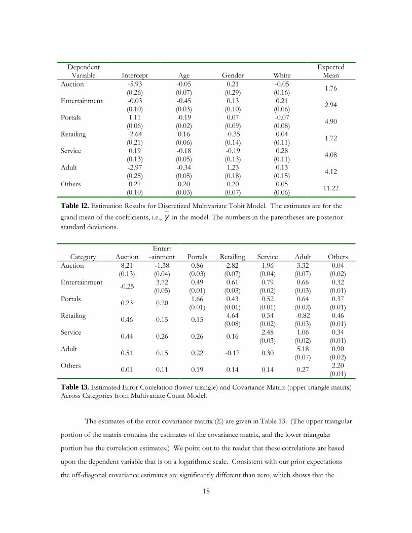
18

Dependent

Variable Intercept Age Gender White Expected

Mean Auction -5.93

(0.26) -0.05 (0.07)

0.21 (0.29)

-0.05 (0.16) 1.76


-0.45 (0.03)

0.13 (0.10)

0.21 (0.06) 2.94

Portals 1.11 (0.06)

-0.19 (0.02)

0.07 (0.09)

-0.07 (0.08) 4.90

Retailing -2.64 (0.21)

0.16 (0.06)

-0.35 (0.14)

0.04 (0.11) 1.72

Service 0.19 (0.13)

-0.18 (0.05)

-0.19 (0.13)

0.28 (0.11) 4.08

Adult -2.97 (0.25)

-0.34 (0.05)

1.23 (0.18)

0.13 (0.15) 4.12

Others 0.27 (0.10)

0.20 (0.03)

0.20 (0.07)

0.05 (0.06) 11.22

Table 12. Estimation Results for Discretized Multivariate Tobit Model. The estimates are for the grand mean of the coefficients, i.e., γ in the model. The numbers in the parentheses are posterior standard deviations.

Category Auction Entert

-ainment Portals Retailing Service Adult Others Auction 8.21

(0.13) -1.38 (0.04)

0.86 (0.03)

2.82 (0.07)

1.96 (0.04)

3.32 (0.07)

0.04 (0.02)

Entertainment -0.25 3.72 (0.05)

0.49 (0.01)

0.61 (0.03)

0.79 (0.02)

0.66 (0.03)

0.32 (0.01)

Portals 0.23 0.20 1.66 (0.01)

0.43 (0.01)

0.52 (0.01)

0.64 (0.02)

0.37 (0.01)

Retailing 0.46 0.15 0.15 4.64 (0.08)

0.54 (0.02)

-0.82 (0.03)

0.46 (0.01)

Service 0.44 0.26 0.26 0.16 2.48 (0.03)

1.06 (0.02)

0.34 (0.01)

Adult 0.51 0.15 0.22 -0.17 0.30 5.18 (0.07)

0.90 (0.02)

Others 0.01 0.11 0.19 0.14 0.14 0.27 2.20 (0.01)

Table 13. Estimated Error Correlation (lower triangle) and Covariance Matrix (upper triangle matrix) Across Categories from Multivariate Count Model.

The estimates of the error covariance matrix (Σ) are given in Table 13. (The upper triangular

portion of the matrix contains the estimates of the covariance matrix, and the lower triangular

portion has the correlation estimates.) We point out to the reader that these correlations are based

upon the dependent variable that is on a logarithmic scale. Consistent with our prior expectations

the off-diagonal covariance estimates are significantly different than zero, which shows that the

19

independence assumption of the univariate model is indeed too strong. Also we find that the

variance estimates of the discretized multivariate tobit model tends to be larger than those of the

discretized, univariate tobit in section 3.4. More substantially we find that auction viewings tend to

occur with retailing, service, and adult viewings indicating some complementary in usage, while

auction viewings tend to substitute for entertainment viewings. This indicates auctions might serve

an entertainment purpose for users. There is also some evidence that retailing and adult viewings

tend to occur in different sessions. For the most part viewing in one category tends to be positively

correlated with unexplained usage in other categories, indicating that during longer sessions

individuals tend to view more viewings from all categories.

4.2. Multivariate Count Model with Mixture Process A final characteristic of our data is that users may exhibit persistence in their viewings. For

example, a user may repeatedly search for price and product information on a retailer site across a

number of sessions. Another user may search for several session for new content and information

until she finds it, and then focuses her attention on the new content that is found. The model

proposed in section 4.1 assumes that each of the sessions are independent of one another. In order

to introduce some dependency across sessions, we propose that user sessions will be drawn from a

mixture process where the transitions between these states follow a markov process. Formally we

can write our model as:

≤

+<≤>==

0 if 0

1ln ln and 0 if ))(exp(*

***

ict

ictictictict Z

) (kZkZZFloorkZ (16)

1such that py probabilit with ],,0[~ ,'1s

ss* =Σ+= ∑

=

S

sitsictsiicsict PMVNXZ εεγ (17)

Where s denotes the state of hidden Markov chain Di. We assume that this hidden Markov chain

follows a continuous-time Markov chain with S states.

We assume that the hidden Markov process Di has the same transition probability matrix P

and the same starting probabilities v across all the users and categories.

and

0

00

0

2

1

321

33231

22321

11312

=

=

SSSS

S

S

S

vv

v

PPP

PPPPPPPPP

P

νo

m

orooo

m

m

m

(18)

20

The hidden Markov chain has waiting times that are exponentially distributed with intensity ),...,1 S (ss =λ .

In order to identify the states of icsγ , we place a restriction on the means of the latent

variable *ictsZ . Specifically, we introduce a variety score, itsR , which is meant to capture the diversity

of the content viewed during the session:

s tci,ZZR iktskictsits and , for ,|))(maxmax(| ** −= (19)

Where *ictsZ is the mean of *

ictsZ . We assume state 1 is the state that exhibits the highest variety-

browsing behavior (lowest value of itsR ) and state S is the state that exhibits the most focus-

browsing behavior (highest value of itsR ): 1)1( itSititS RRR ≥⋅⋅⋅≥≥ − , for i and t.

Given the nature of portals and other sites, users visiting sites in these two categories are more

likely to search for information in other categories and more likely to be in a variety-browsing state.

Therefore, we add another identification condition that is *1'

*)1('

*' ticStictSic ZZZ ≥⋅⋅⋅≥≥ − for i and t,

where c’ = portals or other. We can compute the variety scores from the rest of five categories and apply the restriction, 1)1( itSititS RRR ≥⋅⋅⋅≥≥ − , for i and t, accordingly.

The prior for the continuous-time hidden Markov chain iD is given by:

])(exp[))()((),,|(0

0 ∑ ∫∏∏ =−=≠ s

T

itss

Ms

ls

Nslici dssDIPDvvPDf isisl λλλ (20)

Where v is the density of the starting values of D, where islN is the number of times that Di jumps

from state s to l and where Mis is the number of times that Di jumps to state s , and )( sDI i = is

an indicator function. We refer the reader to Appendices A and B for a discussion of our estimation

procedure.

To better illustrate the movement of our hidden Markov chain, we plot the predicted

probability of being in the focus-browsing state (i.e., state 2) and compare it to an estimate of the

movement based on an ad hoc rule. We select a user with 140 sessions (see Figure 5). Our ad hoc

rule computes the variety score using the function defined in equation (19), but instead of using the

mean of the latent variable we replace it with the observed usage. The ad hoc rule works as follows, if

the variety score for a particular user at a particular time is less than the grand mean of all the variety

scores across users and across time, then the state for that particular user at the particular time is

assigned as state 1—the variety-browsing state; otherwise, the session is assigned to state 2—the

focus-browsing state. Notice in Figure 5 the light user starts with a focus-browsing state and stays in

this state for quite a while, only occasionally switching to the variety-browsing state. Looking at the

data we find that this user normally focuses on adult sites when he is in the focused-browsing state

21

and only occasionally looks at portal sites, retailing sites and other sites. In general, the prediction of the

chain movement is similar to that based on the ad hoc rule. The major difference is in predicting

when the switches occur. Overall, the ad hoc rule tends to over-predict the switching times.

1.0 10.0 19.0 28.0 37.0 46.0 55.0 64.0 73.0 82.0 91.0 100.0 109.0 118.0 127.0 136.0Session

1.0

1.5

2.00.0

0.2

0.4

0.6

0.8

1.0

Ad.Hoc.Rule by Session

Pred icted.Probability.S ta te .Two by Session

Figure 5. Hidden State Movement for One User with 140 Sessions, ‘the light user’.

4.3. Discussion of the Model with Hidden State Movements The first question in model specification is what is the appropriate number of states for our

model. We compute the Bayes factors following Kass and Raferty (1995) for a three different

models: a one state, two state and three state version of the hidden Markov chain model. The two

state model is favored over the one state model by odds of 128243.8. Also, the two state model is

favored over the three state model by odds of 1265.5. Since the two-state Markov process is strongly

favored, we only present the results for this model.

The estimates for the parameters of the two-state model are given in Table 14 and the error

covariance matrix for the two states is given in Table 15. If we look at the intercepts across the

seven categories, which are related to the average tendency to view a page within each category, we

find that in the variety-browsing state portals and other sites are the most likely to be visited. As we

compare these estimates with those in the second state what is most striking is the drop in values for

viewings in the auction, adult, and retail categories. It is important to remember that the expectation

is a function of both the intercept and variance parameters since our latent values have a log

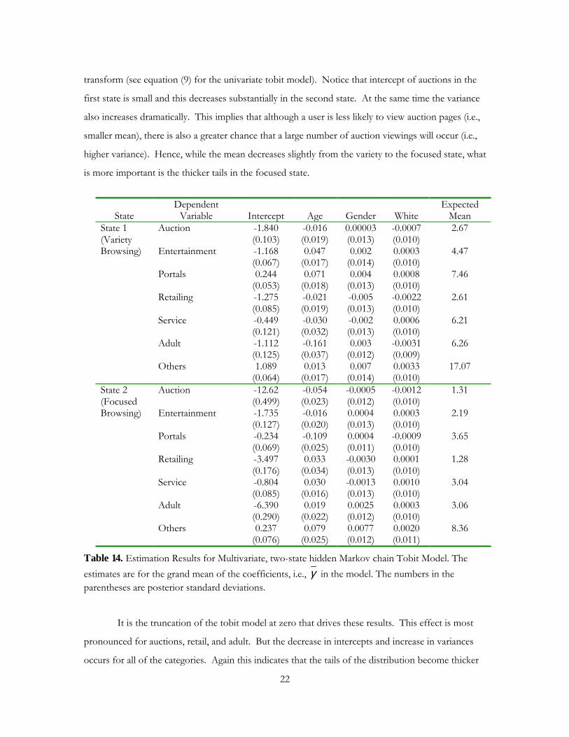
22

transform (see equation (9) for the univariate tobit model). Notice that intercept of auctions in the

first state is small and this decreases substantially in the second state. At the same time the variance

also increases dramatically. This implies that although a user is less likely to view auction pages (i.e.,

smaller mean), there is also a greater chance that a large number of auction viewings will occur (i.e.,

higher variance). Hence, while the mean decreases slightly from the variety to the focused state, what

is more important is the thicker tails in the focused state.

State Dependent

Variable Intercept Age Gender White Expected

Mean Auction -1.840

(0.103) -0.016 (0.019)

0.00003 (0.013)

-0.0007 (0.010)

2.67


0.047 (0.017)

0.002 (0.014)

0.0003 (0.010)

4.47

Portals 0.244 (0.053)

0.071 (0.018)

0.004 (0.013)

0.0008 (0.010)

7.46

Retailing -1.275 (0.085)

-0.021 (0.019)

-0.005 (0.013)

-0.0022 (0.010)

2.61

Service -0.449 (0.121)

-0.030 (0.032)

-0.002 (0.013)

0.0006 (0.010)

6.21

Adult -1.112 (0.125)

-0.161 (0.037)

0.003 (0.012)

-0.0031 (0.009)

6.26

State 1 (Variety Browsing)

Others 1.089 (0.064)

0.013 (0.017)

0.007 (0.014)

0.0033 (0.010)

17.07

Auction -12.62 (0.499)

-0.054 (0.023)

-0.0005 (0.012)

-0.0012 (0.010)

1.31


-0.016 (0.020)

0.0004 (0.013)

0.0003 (0.010)

2.19

Portals -0.234 (0.069)

-0.109 (0.025)

0.0004 (0.011)

-0.0009 (0.010)

3.65

Retailing -3.497 (0.176)

0.033 (0.034)

-0.0030 (0.013)

0.0001 (0.010)

1.28

Service -0.804 (0.085)

0.030 (0.016)

-0.0013 (0.013)

0.0010 (0.010)

3.04

Adult -6.390 (0.290)

0.019 (0.022)

0.0025 (0.012)

0.0003 (0.010)

3.06

State 2 (Focused Browsing)

Others 0.237 (0.076)

0.079 (0.025)

0.0077 (0.012)

0.0020 (0.011)

8.36

Table 14. Estimation Results for Multivariate, two-state hidden Markov chain Tobit Model. The estimates are for the grand mean of the coefficients, i.e., γ in the model. The numbers in the parentheses are posterior standard deviations.

It is the truncation of the tobit model at zero that drives these results. This effect is most

pronounced for auctions, retail, and adult. But the decrease in intercepts and increase in variances

occurs for all of the categories. Again this indicates that the tails of the distribution become thicker

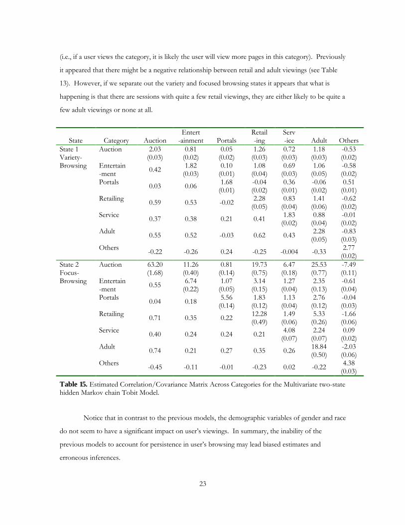
23

(i.e., if a user views the category, it is likely the user will view more pages in this category). Previously

it appeared that there might be a negative relationship between retail and adult viewings (see Table

13). However, if we separate out the variety and focused browsing states it appears that what is

happening is that there are sessions with quite a few retail viewings, they are either likely to be quite a

few adult viewings or none at all.

State Category Auction Entert

-ainment Portals Retail -ing

Serv -ice Adult Others

Auction 2.03 (0.03)

0.81 (0.02)

0.05 (0.02)

1.26 (0.03)

0.72 (0.03)

1.18 (0.03)

-0.53 (0.02)

Entertain -ment 0.42 1.82

(0.03) 0.10

(0.01) 1.08

(0.04) 0.69

(0.03) 1.06

(0.05) -0.58 (0.02)

Portals 0.03 0.06 1.68 (0.01)

-0.04 (0.02)

0.36 (0.01)

-0.06 (0.02)

0.51 (0.01)

Retailing 0.59 0.53 -0.02 2.28 (0.05)

0.83 (0.04)

1.41 (0.06)

-0.62 (0.02)

Service 0.37 0.38 0.21 0.41 1.83 (0.02)

0.88 (0.04)

-0.01 (0.02)

Adult 0.55 0.52 -0.03 0.62 0.43 2.28 (0.05)

-0.83 (0.03)

State 1 Variety- Browsing

Others -0.22 -0.26 0.24 -0.25 -0.004 -0.33 2.77 (0.02)

Auction 63.20 (1.68)

11.26 (0.40)

0.81 (0.14)

19.73 (0.75)

6.47 (0.18)

25.53 (0.77)

-7.49 (0.11)

Entertain -ment 0.55 6.74

(0.22) 1.07

(0.05) 3.14

(0.15) 1.27

(0.04) 2.35

(0.13) -0.61 (0.04)

Portals 0.04 0.18 5.56 (0.14)

1.83 (0.12)

1.13 (0.04)

2.76 (0.12)

-0.04 (0.03)

Retailing 0.71 0.35 0.22 12.28 (0.49)

1.49 (0.06)

5.33 (0.26)

-1.66 (0.06)

Service 0.40 0.24 0.24 0.21 4.08 (0.07)

2.24 (0.07)

0.09 (0.02)

Adult 0.74 0.21 0.27 0.35 0.26 18.84 (0.50)

-2.03 (0.06)

State 2 Focus- Browsing

Others -0.45 -0.11 -0.01 -0.23 0.02 -0.22 4.38 (0.03)

Table 15. Estimated Correlation/Covariance Matrix Across Categories for the Multivariate two-state hidden Markov chain Tobit Model.

Notice that in contrast to the previous models, the demographic variables of gender and race

do not seem to have a significant impact on user’s viewings. In summary, the inability of the

previous models to account for persistence in user’s browsing may lead biased estimates and

erroneous inferences.

24

The estimates for the two-state hidden Markov chain are given in Table 16. Notice that the

user has a high probability of starting in a variety browsing state (89%). These sessions tend to have

a smaller number of viewings in many categories. On average the user will stay in this variety-

browsing state for about two sessions (i.e., the inverse of waiting time is 0.56). In contrast the

focused browsing states tend to carry over a longer period time of about four sessions (i.e., the

inverse of waiting time is 0.25). The transition probability matrix is trivial for the two-state model,

since there are only two states and the switching behavior is captured by the waiting time in each

state.

State 1 (Variety-Browsing) State 2 (Focus-Browsing) λ (Inverse of Waiting Time) 0.56

(0.005) 0.25

(0.007) ν (Starting Probabilities) 0.89

(0.018) 0.11

(0.018) 0 1 P (Transition Probabilities) 1 0

Table 16. Estimation Results for the Two-State Hidden Markov Chain

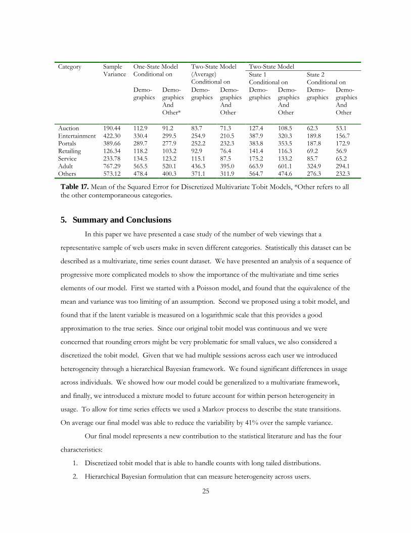
A final analysis was preformed to understand the contribution in terms of predictive ability

of our final model using various information sets. The results are provided in Table 17. First we

calculate the sample variance of the original dataset as given in Table 3. Next we estimate our one-

state model (which is the same as the model presented in section 4.1) using the demographic

information. For example, the sample variance of retailing viewings is 126.34, but by using the one-

state model estimates and the demographics this is reduced by 6% to 118.2. In the next column we

predict the number of retail viewings in a session using the one-state model estimates and assuming

that we know the demographics and the viewings in all the other categories. For the retailing

category we find that the variance is reduced by 18% if we know the viewings in the other categories.

We then repeat these calculations using our two-state model, and find that with demographics and

the other categories we can reduce the variance by 40%. To help understand these gains we show

the variability in each of the states in the final four columns. Much of the gain comes from being

able to know if the user is in a focused or variety seeking state. The gains in the other categories are

even more dramatic. On average our one state model reduces the variance by 26%, and the two state

model by 41%. If we have information about the viewings in the other categories we can reduce the

variance by about half (50%).

25

Two-State Model One-State Model

Conditional on Two-State Model (Average) Conditional on

State 1 Conditional on

State 2 Conditional on

Category Sample Variance

Demo-graphics

Demo-graphics And Other*

Demo-graphics

Demo-graphics And Other

Demo-graphics


Demo-graphics


Auction 190.44 112.9 91.2 83.7 71.3 127.4 108.5 62.3 53.1 Entertainment 422.30 330.4 299.5 254.9 210.5 387.9 320.3 189.8 156.7 Portals 389.66 289.7 277.9 252.2 232.3 383.8 353.5 187.8 172.9 Retailing 126.34 118.2 103.2 92.9 76.4 141.4 116.3 69.2 56.9 Service 233.78 134.5 123.2 115.1 87.5 175.2 133.2 85.7 65.2 Adult 767.29 565.5 520.1 436.3 395.0 663.9 601.1 324.9 294.1 Others 573.12 478.4 400.3 371.1 311.9 564.7 474.6 276.3 232.3

Table 17. Mean of the Squared Error for Discretized Multivariate Tobit Models, *Other refers to all the other contemporaneous categories.

5. Summary and Conclusions In this paper we have presented a case study of the number of web viewings that a

representative sample of web users make in seven different categories. Statistically this dataset can be

described as a multivariate, time series count dataset. We have presented an analysis of a sequence of

progressive more complicated models to show the importance of the multivariate and time series

elements of our model. First we started with a Poisson model, and found that the equivalence of the

mean and variance was too limiting of an assumption. Second we proposed using a tobit model, and

found that if the latent variable is measured on a logarithmic scale that this provides a good

approximation to the true series. Since our original tobit model was continuous and we were

concerned that rounding errors might be very problematic for small values, we also considered a

discretized the tobit model. Given that we had multiple sessions across each user we introduced

heterogeneity through a hierarchical Bayesian framework. We found significant differences in usage

across individuals. We showed how our model could be generalized to a multivariate framework,

and finally, we introduced a mixture model to future account for within person heterogeneity in

usage. To allow for time series effects we used a Markov process to describe the state transitions.

On average our final model was able to reduce the variability by 41% over the sample variance.

Our final model represents a new contribution to the statistical literature and has the four

characteristics:

1. Discretized tobit model that is able to handle counts with long tailed distributions.

2. Hierarchical Bayesian formulation that can measure heterogeneity across users.

26

3. Multivariate formulation that is useful when the underlying counts are interdependent.

4. Mixture model with Markov process that can describe within person heterogeneity and

persistence or time series effects in the underlying process.

Although we have reserved the discussion of the estimation procedure for the Appendix, we have

employed several recent advances in the statistical literature: Markov Chain Monte Carlo estimation

algorithm, slice sampler for truncated distributions, and reversible jump for estimating the switching

model. Without these new techniques it would have been quite difficult to estimate our new

proposed model.

Besides the methodological contribution, we have also learned about web browsing

behavior:

1. The marginal distribution of web viewing during a session has a long-tail. This distribution

also has many observations that are zeroes (See Figure 3).

2. If an analyst only looks naively at the sample correlation matrix (Table 4) it may appear that

the counts of viewings in each category are independent of one another. However, this

is not the case. In our analysis we found that the long-tail, high frequency of censored

observations, and heterogeneity masked the correlations amongst the counts (see Table

13 and 15).

3. Our final model can explain about half the sample variance if we know the viewings in the

other categories and the user’s demographics.

4. Users tend to have sessions that are focused on viewing a variety of information, and then

switch to sessions that are more narrowly focused on viewing information from fewer

categories.

We believe these findings will be of interest to web designers, marketing researchers, and cognitive

psychologists. First, for web designers it implies that knowing the context of a visit (what else did

the user do during their session) could potentially be very useful in understanding how long a user

will stay at a site. Marketing researchers should be interested to know that 40% of the variability of

retail visits can be explained by user demographics and viewings in other categories. This could

potentially help marketers better target users who are interested in shopping, and help eliminate some

of the unwanted advertising of those users who are not interested in shopping. Finally, our results

support the foraging model of information search proposed by cognitive psychologists. It appears

that users graze across many sites (or information sources), and then narrowly browse fewer

27

categories but in more depth. For information rich environments like the web, foraging models may

be efficient strategies for users in locating and using information.

Appendix A: Estimation Notes


We use a standard Bayesian approach (Gibbs Sampler) to estimate our discretized tobit

model by assuming the following diffuse priors:

]001.0 ,1[~.000,000,1 . and ,for , ..., 1,

covariate, for thet coefficien thedenotes where],,0[ ~

2

2

thth2

maInverseGamlciLl

lllN

c

cl

clcl

σσ

σγ

==

Hierarchical Bayesian Formulation of the Discretized Univarite Tobit Model with Log

Transformation

In the last univariate count model that we add heterogeneity to the discretized Type I Tobit

model with log transformation. We employ an exchangeable prior to induce shrinkage across users

with the following prior setup:

]001.0 ,1[~. and for ],001.0 ,1[~

. and for ],1000000 ,0[~

. and ,for , ..., 1, covariate, for thet coefficien thedenotes where],,[ ~

2

2

thth2

maInverseGamlcmaInverseGam

lcN

lciLllllN

c

cl

cl

clclicl

σσ

γ

σγγ=

Since the full conditional distributions for the parameters in the two discretized tobit models

are relatively straightforward, we do not include them in this paper. Those who are interested in them

may consult with Appendix B where the full conditional distributions for the multivariate tobit model

with mixture process are specified.

28

Hierarchical Bayesian Formulation of the Discretized Multivariate Tobit Model with Log

Transformation and Markov Mixture Process We assume a priori that the densities of the starting values for Di, )( 0iDv , and the density of

each row of the hidden chain transition matrix are Dirichlet densities. In addition, we assume a priori that the intensity parameters, sλ , for Di follow a Gamma density. That is,

P of row j theis vector,C1 a is ],[~

),(~)(~

thjjjj

priorpriors

PDirichletP

scaleshapeGammaDirichletv

×ττ

λα

We complete the rest of the model with the following priors.

],[~

l. and sfor ],,[~

l. and sfor ],1,0[~

l. and s i,for ,L ..., 1, l covariate, l for the tscoefficien of vector l thedenotes l where],,[ ~

1

1

thth

ΣΣ−

−

Σ

Ω

⋅

=

VWishartWishartV

IMVN

VMVN

s

vsl

sl

slslisl

ρρ

δγ

γγ

Notice that a Bayesian shrinkage approach is used to account for consumer heterogeneity.

We apply data augmentation and MCMC method (Gibbs Sampler and Reversible Jump Algorithms)

based on the following full conditional distributions.

,,| ,|

,,,,,|

,| ,,,,|

,,,|

one the

except covariates allfor denotes where,,,,,,|

,,|

,,,|

*

s

*1-

1

*

*

jij

i

jislsiiti

priorpriori

iislits

vslislsl

th

-sslsliislitisl

slislsl

siislitit

vDPDv

PvXZD

, scale shapeDVXZ

V

l

lVXZ

V

XZZ

τα

γ

λργ

ργγ

γγγ

δγγ

γ

Σ

Σ

Ω

Σ

Σ

ΣΣ

−

−

The multivariate draws of *itZ are generated from truncated normal distribution using a Slice

Sampler. The multivariate draws of slγ and islγ are generated from conjugate multivariate normal

distributions given the identifiability restrictions. The random draws of -1sΣ and 1−

slV are generated

from conjugate Wishart distributions. The random draws of sλ are generated from a conjugate

29

Gamma distribution. We generate the draws of iD using a reversible jump algorithm. The

multivariate draws of v and jP are generated from conjugate Dirichlet distributions. The

estimation procedure was coded using a C++ program. The first 10,000 iterations are discarded as a

“burn-in” period after convergence of the chains was observed, and the last 5,000 iterations are used

to compute the posterior moments.

Appendix B: Monte Carlo Markov Chain for Estimating the Model

The full conditional distributions are given as follows. (1). Data augmentation step: The full conditional density for *Zict

can be sampled from using a slice

sampler algorithm, see Damian and Walker (1999) for a general discussion of the slice sampler

algorithm.

it

cjcj

cjcj

it

DsssdiagI

otherwiseiXijsijtZiXicsN

ictZiXijsijtZiXicskkN

DsiXicsictZtcjiZictZ

=ΣΣ−=Ξ

Ξ−Ξ+−∞

>Ξ−Ξ++

Σ≠

−−−

≠

≠

∑

∑

and ,)]([ Where

])( ,)'*('[]0,(

0 if ])( ,)'*('[))1ln(,[ln~

,,,,,*,,|*

111

cc1-

cc1-

γγ

γγ

γ

(2). ]A ),([ ~ ,,| 1

∑−⋅

iislslslislsl VAMVNV γδγγ

Where 11 )( −− ⋅+= ∑ IVAi

sl δ .

(3).

]))`'*)('*(( ,[ ~

,,,,*|

1

1 1

1-

−

= =ΣΣ

ΣΣ

∑∑ −−++

ΣI

i

T

tiisiis

iisls

XitZXitZVITWishart

VXitZ

γγρ

ργ

(4).

and I

]B ),'([ ~ ,,,,,,*|

*1'

*)1('

*'1)1(

11

ticStictSicitSititS

slslt

itlsilisslsliislisl

ZZZRRR

VZXBMVNDVXitZ

≥⋅⋅⋅≥≥≥⋅⋅⋅≥≥

+Σ⋅Σ

−−

−−∑− γγγγ

30

Where 111 )'( −−− +Σ= ∑ slt

ilsil VXXB , −−−= ilislitl XitZZ '* γ , I. is an indicator function, c’ =

portals or other, and 2 1orr = .

(5).

]))'-)(-(( ,[

~ ,,,|1I

1i

1

−

=

−

∑+Ω+

Ω

slislslislv

vslislsl

IWishart

V

γγγγρ

ργγ

(6) ),(~,,| prior

icsprior

icspriorprioris scaleTshapenGammascaleshapeD ++ ∑∑λ

where ns is the number of times Di was in state s and Ts is the amount of time that Di was in state s.

(7).

,,,,,*| jislsii PvXitZD γΣ ~ Reversible Jump Algorithm: independence sampler,

refinement sampler, and birth-and-death sampler. We use the reversible jump Hasting Metropolis

(HM) algorithms proposed by Liechty and Roberts (2001) to generate samples of each hidden

Markov chain Di. The difference between their algorithm and ours is based on the distribution of Z

in this paper versus the likelihood functions in theirs. We used three different algorithms for

updating Di. The first algorithm is an independence algorithm, which ignores the current realization

of Di and proposes realizations of Di by drawing from the prior density of Di. This results in

proposed realizations that are considerably different, in terms of the posterior density, and as a

consequence this algorithm tends to result in large but infrequent moves. The other two algorithms

create proposed realizations of Di by making small modifications to the current realization of Di.

The second algorithm is a refinement algorithm where the proposed realization of Di is created by

modifying one of the jump times of the current realization of Di. The third algorithm is a birth-

death algorithm where the proposed realization of Di is created by either inserting a new interval into

the current realization of Di – a birth – or removing an interval from the current realization of Di – a

death. The independence algorithm has obvious advantages when the posterior distribution is multi-

modal or when a poor initial value of Di has been chosen, where as the refinement algorithm and the

birth-death algorithm have the advantage of more efficiently exploring the modes of the posterior

31

distribution. In order to take advantage of the properties of these three algorithms, one of these three

algorithms is randomly chosen at each iteration of the MCMC algorithm to update each hidden

Markov chain. Although our model itself is different from theirs, we apply the algorithms proposed

by Liechty and Roberts (2001) and refer to their description of the algorithms and the formulas for

calculating the acceptance probabilities.

(8).

=

=++ ∑∑∑=

otherwise 0user ifor s isstatestarting if1

1 with , ... , ~,|S

1j11

is

ji

iSSi

ii

dwhere

v)ddDirichlet(Dv ααα

(9).

user i.for k state to j state from jumps ofnumber the is

1 with , ... ,~ ,,|1

11

ijk

S

kijk

iijSjS

iijjjij

mwhere

P)mmDirichlet(vDP =++ ∑∑∑=

τττ

The draws of Pj can be sampled from Gamma distribution with ∑+=i

ijkjk mshape τ and scale =

1 for all k. Then normalize each draw using the sum of all of the draws.

32

References

Allenby, G. M., Arora, N., and Ginter, J. L. (1998), “On the Heterogeneity of Demand,” Journal of Marketing Research, 35 (3), 384-389.

Aitchison, J., and Ho, C. H. (1989), “The Multivariate Poisson-Log Normal Distribution,” Biometrika, 76, 4, 643-653.

Blundell, R., Griffith, R., and Reenen, J. V. (1995), “Dynamic Count Data Models of Technological Innovation,” The Economic Journal, 105, 429, 333-344.

Boswell, M. T., and Patil, G. P. (1970), “Chance Mechanisms Generating the Negative Binomial Distributions,” in G. Patil (ed.), Random Counts in Models and Structures: Volume 1, The Pennsylvania State University Press, Pennsylvania.

Brännäs, K. (1992), “Limited Dependent Poisson Regression,” The Statistician, 41, 413-423.

Bucklin, R., and Sismeiro, C. (2001), “A Model of Website Browsing Behavior Estimated on Clickstream Data,” UCLA Working Paper.

Cadez, I.V., D. Heckerman, C. Meek, P. Smyth, and S. White (2000), “Visualzation of Navigation Patterns on a Web Site Using Model Based Clustering”, in Proceedings of the KDD 2000, pp. 280-284.

Cameron, A. C., and Trivedi, P. K. (1986), “Econometric Models Based on Count Data: Comparisons and Applications of Some Estimators and Tests,” Journal of Applied Econometrics, 1, 29-53.

Coffey, S. (1999), “Media Metrix Methodology,” Media Metrix Working Paper, http://www.mediametrix.com/Methodology/Convergence.html

Damien, P. S., J. Wakefield, and G. Walker (1999), “Gibbs Sampling For Bayesian Nonconjugate and Hierarchical Models Using Auxilliary Variables,” Journal of Royal Statistical Society, Series B, 61, Part 2, 331-344.

Desphande, M. and G. Karypis (2000), “Selective Markov Models for Predicting Web-Page Accesses”, in First International SIAM Conference on Dataming.

Farewell, V. T., and Sprott, D. A. (1988), “The Use of a Mixture Model in the Analysis of Count Data,” Biometrics, 44, 1191-1194.

Gooley, C.G. and J. M. Lattin (2001), “Dynamic Customization of Marketing Messages in Interactive Media”, Working Paper, Graduate School of Business, Stanford University.

Grogger, J. T., and Carson, R. T. (1991), “Models for Truncated Counts,” Journal of Applied Econometrics, 6, 225-238.

Gönül, F., and Srinivasan, K. (1993), “Modeling Multiple Sources of Heterogeneity in Multinomial Logit Models: Methodological and Managerial Issues,” Marketing Science, 12 (3), 213-229.

Huberman, B. A., Pirolli, P. L. T., Pitkow, J. E., and Lukose, R. M. (1998), “Strong Regularities in World Wide Web Surfing,” Science, 280, 95-97.

Johnson, E. J., Moe, W. W., Fader, P. S., Bellman, S., and Lohse, J. "On the Depth and Dynamics of World Wide Web Shopping Behavior," Wharton Marketing Department Working Paper #00-019.

Liechty, J. C. & G. O. Roberts (2001). Markov Chain Monte Carlo Methods for Switching Diffusion

Models. Biometrika, 88 2, pp. 299-315 .

33

Moe, W., W. and Fader, P. S. (2001), “Which Visits Lead to Purchase? Dynamic Conversion Behavior at e-Commerce Sites,” Wharton Marketing Department Working Paper #00-023.

Montgomery, A. L. and Faloutos, C. (2002), “Using Clickstream Data to Identify World Wide Web Browsing Trends,” GSIA Working Paper 2000-E20.

Nielsen, J. (2000), Designing Web Usability: The Practice of Simplicity, New Riders Publishing.

Patil, G. P. (1970), Random Counts in Models and Structures: Volume 1, The Pennsylvania State University Press, Pennsylvania.

Pirolli, P. and S.K. Card (1999), “Information Foraging”, Psychological Review, 106(4): 643-675.

Ramaswamy, V., Anderson, E. W., and Desarbo, W. S. (1994), “A Disaggregate Negative Binomial Regression Procedure for Count Data Analysis,” Management Science, 40, 3, 405-417.

Rossi, P.E. and G.M. Allenby (2000), “Statistics and Marketing”, Journal of the American Statistical Association, 95, 635-38.

van Duijn, M. A. J., and Böckenholt, U. (1995), “Mixture Models for the Analysis of Repeated Count Data,” Applied Statistics, 44, 4, 473-485.

Wedel, M., Desarbo, W. S., Bult, J. R., and Ramaswamy, V. (1993), “A Latent Class Poisson Regression Model for Heterogeneous Count Data,” Journal of Applied Econometrics, 8, 397-411.

Documents

Modeling Category Viewership of Web Users with Multivariate Count