Basic Statistics - CERN Indico

Basic Statistics

Sadhana Dash

July 16, 2021

Sadhana Dash Basic Statistics July 16, 2021 1 / 72



Outline

ProbabilityRandom Numbers and Probability DensitiesExpectation ValuesSimple Statistical DistributionsCentral Limit Theorem


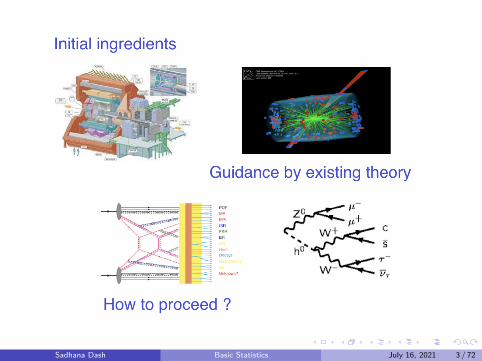
Figure: A schematic of scientific methodSadhana Dash Basic Statistics July 16, 2021 5 / 72

Statistics : DefinitionThe art of learning from data. It is concerned with the collection of data,its subsequent description, and its analysis, which often leads to thedrawing of conclusions.Two Types :1. Descriptive Statistics : The part of statistics, concerned with thedescription and summarization of data, is called descriptive statistics.2. Inferential Statistics : The part of statistics, concerned with thedrawing of conclusions, is called inferential statistics.

Figure: Descriptive versus Inferential statistics


Population and Sample

Figure: A schematic of population and sample

Population is the entire set of possible cases for which a study isconducted.Sample refers to a subgroup of population from which we try to learnabout the population.A measure concerning a population is called parameter while that of asample is called a statistic.


Sample Spaces and Events

Random Experiment : An experiment that can result in differentoutcomes, even though it is repeated in similar manner every time, iscalled a random experiment.Sample Space : The set of all possible outcomes of a random experimentis called the sample space of the experiment. The sample space is denotedas SExample : Consider an experiment in which the thickness of a siliconwafer is measured and a test is carried out to see whether it conforms tothe required specifications or not. The outcome can be yes or no. If twowafers are selected, the sample space can be represented byS = (yy , yn, ny , nn)Roll a fair dice. The sampl e space consists ofS = (1, 2, 3, 4, 5, 6)Event : An event is a subset of the sample space of a random experiment .


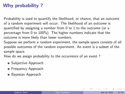
Why probability ?

Probability is used to quantify the likelihood, or chance, that an outcomeof a random experiment will occur. The likelihood of an outcome isquantified by assigning a number from 0 to 1 to the outcome (or apercentage from 0 to 100%). The higher numbers indicate that theoutcome is more likely than lower numbers.Suppose we perform a random experiment, the sample space consists of allpossible outcomes of the random experiment. An event is a subset of thesample space.How do we assign probability to the occurrence of an event ?

Subjective Approach

Frequency Approach

Bayesian Approach


Axioms of Probability

Probability is a number that is assigned to each member of a collection ofevents from a random experiment that satisfies the following properties: IfS is the sample space and E is any event in a random experiment,

P(S) = 1

0 ≤ P(E ) ≤ 1

If two events E1 and E2, which have no outcomes in common ,P(E1UE2) = P(E1) + P(E2)


Conditional Probability

The conditional probability of an event F given an event E has alreadyoccurred, denoted by P(F |E ) , is given byP(F |E ) = P(E ∩ F )/P(E ) , for P(E ) > 0The validity of the definition can be easily shown for a special case inwhich all outcomes of a random experiment are equally likely.If there are n outcomes,P(E ) = number of outcomes in E

n

P(E ∩ F ) = number of outcomes in E ∩ Fn

Therefore, P(E∩F )P(E) = number of outcomes in E ∩ F

number of outcomes in E

Hence, P(F |E ) can be interpreted as the relative frequency of event Famong the trials that produce an outcome in event E.


Multiplication Rule

The general expression for the probability of the intersection of two eventsis called the multiplication rule for probabilities.P(E ∩ F ) = P(F |E )P(E ) = P(E |F )P(F )Total Probability Rule For any two events E and F , one can express E asE = (E ∩ F ) ∪ (E ∩ F

′)

The value to be in event E, it must be either in both E and F or be in Ebut not in F. As EF and EF

′are mutually exclusive sets, one can write

that P(E ) = P(E ∩ F ) + P(E ∩ F′)

= P(E |F )P(F ) + P(E |F ′)P(F′)

The above expression can be generalized for k mutually exclusive andexhaustive sets. If F1, F2, .., Fk are k mutually exclusive and exhaustivesets, thenP(E ) = P(E ∩ F1) + P(E ∩ F2) + ...+ P(E ∩ Fk)= P(E |F1)P(F1) + P(E |F2)P(F2).+ ....+ P(E |Fk)P(Fk)


Baye’s Theorem

According to the definition of conditional probability,P(E ∩ F ) = P(F |E )P(E ) = P(E |F )P(F )We can writeP(E |F ) = P(F |E)P(E)

P(F ) , for P(F ) > 0If E1,E2, ..,Ek are k mutually exclusive and exhaustive sets and F is anyevent,P(E1|F ) = P(F |E1)P(E1)

P(F |E1)P(E1)+P(F |E2)P(E2).+....+P(F |Ek )P(Ek ) , for P(F ) > 0

Example: Consider a beam which has 90% pions and 10% kaons. Thekaons have 95% probability of giving no Cherenkov signal while pions have5% probability of giving none. What is the probability that a particle thatgave no signal is a kaon?


Bayesian Philosophy

P(Theory |Data) = P(Data|Theory)P(Theory)P(Data)

Posterior ∼ Likelihood × Prior


Random Variable : Definition

A Random Variable is a variable that associates a number with theoutcome of a random experiment.A Random variable is a function that assigns a real number to eachoutcome in the sample space of a random experiment.They are generally denoted by upper case alphabets X or Y to distinguishfrom algebraic variables.After an experiment is conducted, the measured value of the randomvariable is denoted by a lower case letter.The range of a random variable X, shown by Range(X) or RX , is the setof possible values of X.


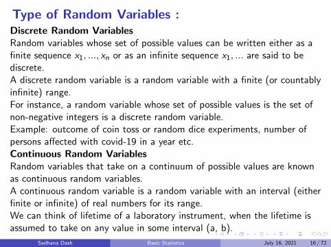
Type of Random Variables :Discrete Random VariablesRandom variables whose set of possible values can be written either as afinite sequence x1, ..., xn or as an infinite sequence x1, ... are said to bediscrete.A discrete random variable is a random variable with a finite (or countablyinfinite) range.For instance, a random variable whose set of possible values is the set ofnon-negative integers is a discrete random variable.Example: outcome of coin toss or random dice experiments, number ofpersons affected with covid-19 in a year etc.Continuous Random VariablesRandom variables that take on a continuum of possible values are knownas continuous random variables.A continuous random variable is a random variable with an interval (eitherfinite or infinite) of real numbers for its range.We can think of lifetime of a laboratory instrument, when the lifetime isassumed to take on any value in some interval (a, b).


Probability DistributionsThe probability distribution of a random variable X is a description of theprobabilities associated with the possible values of X.Probability Mass Function (PMF) For a discrete random variable Xwith possible values x1, x2, ..xn, a probability mass function is a functionsuch that

f (xi ) ≥ 0∞∑i=0

f (xi ) = 1

f (xi ) = P(X = xi )

Figure: PMF of a discrete random variable


Cumulative Distribution Function (CDF) ofDiscrete random variable

The cumulative distribution function ( or simply the distribution function )of a discrete random variable X, denoted as F(x), is the probability thatthe random variable X takes on a value that is less than or equal to xF (x) = P(X ≤ x) =

∑xi≤x

f (xi )

For a discrete random variable X, F(x) satisfies the following properties.

F (x) = P(X ≤ x) =∑xi≤x

f (xi )

0 ≤ F (x) ≤ 1

If x ≤ y, then F(x) ≤ F(y)


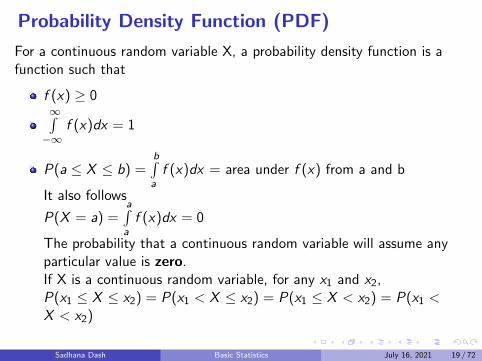
Probability Density Function (PDF)

For a continuous random variable X, a probability density function is afunction such that

f (x) ≥ 0∞∫−∞

f (x)dx = 1

P(a ≤ X ≤ b) =b∫af (x)dx = area under f (x) from a and b

It also follows

P(X = a) =a∫af (x)dx = 0

The probability that a continuous random variable will assume anyparticular value is zero.If X is a continuous random variable, for any x1 and x2,P(x1 ≤ X ≤ x2) = P(x1 < X ≤ x2) = P(x1 ≤ X < x2) = P(x1 <X < x2)


The cumulative distribution function (cdf) of a continuous randomvariable X is

F (a) = P(X < a) =a∫−∞

f (x)dx , for −∞ < a <∞

Differentiating both the sides:ddaF (a) = f (a)

Figure: (Left panel) : PDF (Right panel) : CDF of a continuous random variable

P

{a− ε/2 ≤ X ≤ a + ε/2

}=

a+ε/2∫a−ε/2

f (x)dx ∼ εf (a) when ε is small. In

other words, the probability that X will be contained in an interval oflength ε around the point a is approximately εf (a).


Expectation Value

If X is a discrete random variable taking on the possible values x1, x2, ..,the mean or expected value of the discrete random variable X, denoted asµ or E[X], isµ = E [X ] =

∑ixi f (xi )

Thus, the expected value of X is a weighted average of the possible valuesthat X can take on, each value being weighted by the probabilityassociated with X.If X is a continuous random variable with the probability density functionf (x), the mean or expected value of X, denoted as E[X ], is given by

µ = E [X ] =∞∫−∞

xf (x)dx


VarianceVariance quantifies the variation, or spread, of the values associated withthe random variable X. It measures the dispersion, or variability in thedistribution.If X is a discrete random variable with mean µ, then the variance of X ,denoted by Var(X ) or σ2, is defined byVar(X ) = σ2 = E [(X − µ)2]=∑x

(x − µ)2f (x) =∑xx2f (x)− µ2

If X is a continuous random variable with probability density function f(x),V(X) or σ2 is defined as

Var(X ) = σ2 =∞∫−∞

(x − µ)2f (x)dx

The standard deviation, σ isσ =√σ2

It can be shownVar(X ) = E [X 2]− µ2

If a and b are constants, Var(aX + b) = a2Var(X )Var(b) = 0


CovarianceThe covariance between the random variables X and Y , denoted ascov(X ,Y ) or σXY , isσXY = Cov(X ,Y ) = E [(X − µX )(Y − µY )]= E[XY] - µxE [Y ]− µyE [X ] + µxµy = E [XY ]− E [X ]E [Y ]σXY = σYXσXX = Var(X )Properties :

Cov(X,X)=Var(X)

Cov(X,Y) = Cov(Y,X)

Cov(aX,Y) = aCov(X,Y)

Cov(X+c,Y) = Cov(X,Y)

Cov(X+Y, Z) = Cov(X,Z) + Cov(Y,Z)Cov(X+Y, Z)= E[(X+Y)Z] - E(X+Y)E[Z]=E[XZ + YZ] - (E[X]+E[Y])E[Z]=E[XZ] - E[X]E[Z] + E[YZ] - E[Y]E[Z]= Cov(X,Z) + Cov(Y,Z)


We can show that

Cov( n∑

i=1Xi ,Y

)=

n∑i=1

Cov(Xi ,Y )

Cov( n∑

i=1Xi ,

m∑j=1

Yj

)=

n∑i=1

m∑j=1

Cov(Xi ,Yj)

Variance of sum of random variables

Var( n∑

i=1Xi

)=

n∑i=1

Var(Xi ) +n∑

i=1

n∑j=1,j 6=i

Cov(Xi ,Xj)

if X and Y are independent, then Cov(X,Y)=0As they are independent, Cov(X.Y) = E[XY] - E[X]E[Y]=E[X]E[Y] - E[X]E[Y] = 0Cov(X,Y) = 0

Therefore, for independent variables X1...Xn, Var( n∑

i=1Xi

)=

n∑i=1

Var(Xi )


Correlation Coefficient

The correlation coefficient, ρXY of two random variables X and Y isobtained by dividing the covariance by the product of standard deviationsof X and Y .ρXY = Corr(X ,Y ) = Cov(X ,Y )

σXσYProperties of the correlation coefficient:

−1 ≤ ρX ,Y ≤ 1

If ρX ,Y = 1, then Y = aX + b, where a > 0

If ρX ,Y = −1, then Y = aX + b, where a < 0

ρ(aX + b, cY + d) = ρ(X ,Y )

If ρ(X ,Y ) = 0, we say that X and Y are uncorrelated.If ρ((X ,Y ) > 0, we say that X and Y are positively correlated.If ρ(X ,Y ) < 0, we say that X and Y are negatively correlated.


Moment Generating function

Moments: Let X be any random variable. The moments are the expectedvalues of various powers of X.E[X] = first momentE[X 2] = second momentE[X k ] = kth momentThe moment generating function (MGF), MX (t) of a random variable X isdefined for all the values of t (provided the expectation exists for some t ina neighbourhood of zero) by

MX (t) = E [etX ] =

∑xetx f (x) , if X is a discrete rv

+∞∫−∞

etx f (x)dx , if X is continuous rv


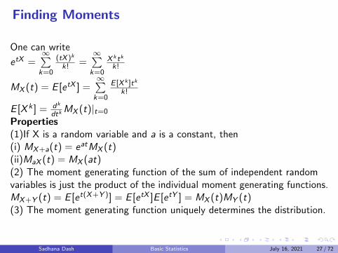
Finding Moments

One can write

etX =∞∑k=0

(tX )k

k! =∞∑k=0

X k tk

k!

MX (t) = E [etX ] =∞∑k=0

E [X k ]tk

k!

E [X k ] = dk

dtkMX (t)|t=0

Properties(1)If X is a random variable and a is a constant, then(i) MX+a(t) = eatMX (t)(ii)MaX (t) = MX (at)(2) The moment generating function of the sum of independent randomvariables is just the product of the individual moment generating functions.MX+Y (t) = E [et(X+Y )] = E [etX ]E [etY ] = MX (t)MY (t)(3) The moment generating function uniquely determines the distribution.


Markov’s Inequality

If X is a random variable that takes only non-negative values, then for anyvalue a > 0P[X ≥ a] ≤ E [X ]

aLet us show when X is a continuous random variable with pdf, f(x)

E [X ] =∞∫0

xf (x)dx

=a∫

0

xf (x)dx +∞∫axf (x)dx

≥∞∫axf (x)dx

≥∞∫aaf (x)dx

= a∞∫af (x)dx = aP[X ≥ a]


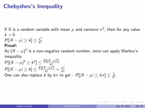
Chebyshev’s Inequality

If X is a random variable with mean µ and variance σ2, then for any valuek > 0P[|X − µ| ≥ k] ≤ σ2

k2

Proof:As (X − µ)2 is a non-negative random number, once can apply Markov’sinequality

P[(X − µ)2 ≥ k2] ≤ E [(X−µ)2]k2

P[|X − µ| ≥ k] ≤ E [(X−µ)2]k2 = σ2

k2

One can also replace k by kσ to get : P[|X − µ| ≥ kσ] ≤ 1k2


The Law of Large Numbers

Let X1,X2, ...Xn , be a sequence of independent and identically distributedrandom variables, each having mean E [Xi ] = µ and variance, σ2. Then,for any ε > 0,P[|X1+...+Xn

n − µ| > ε]→ 0 as n →∞Sequential Deduction : One can show,

E [X1+...Xnn ] = µ

Var(X1+...Xnn ) = σ2

nFrom Chebyshev’s inequality , one can writeP[|X1+...+Xn

n − µ| > ε] ≤ σ2

nε2

which tends to zero as n →∞


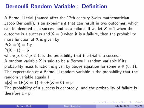
Bernoulli Random Variable : Definition

A Bernoulli trial (named after the 17th century Swiss mathematicianJacob Bernoulli), is an experiment that can result in two outcomes, whichcan be denoted as a success and as a failure. If we let X = 1 when theoutcome is a success and X = 0 when it is a failure, then the probabilitymass function of X is given byP(X =0) = 1-pP(X =1) = pwhere p, 0 < p < 1, is the probability that the trial is a success.A random variable X is said to be a Bernoulli random variable if itsprobability mass function is given by above equation for some p ∈ (0, 1).The expectation of a Bernoulli random variable is the probability that therandom variable equals 1.E[X] = 1P(X = 1) + 0P(X = 0) = pThe probability of a success is denoted p, and the probability of failure istherefore 1 - p.


Binomial Random Variable : Definition

A random experiment consists of n Bernoulli trials such that(1) The trials are independent(2) Each trial results in only two possible outcomes, labeled as success andfailure(3) The probability of a success in each trial, denoted as p, remainsconstantThe random variable X that equals the number of trials that result in asuccess has a binomial random variable with parameters 0 < p < 1 andn = 1, 2, ..... The probability mass function of X isf (x) =

(nx

)· px(1− p)n−x , x = 0,1,2, ...n



Properties of Binomial Random Variable

(1) f (x) > 0

(2)n∑

x=0f (x) =

n∑x=0

(nx

)px(1− p)n−x = [p + (1− p)]n = 1

If X is a binomial random variable with parameters p and n,E (X ) = npWe know that X is the sum of n identical Bernoulli random variables, eachwith expected value p.X = X1 + · · ·+ Xn

From the linearity of the expected valuesE[ X ] = E [X1 + X2 · · ·+ Xn]= E [X1] + · · ·+ E [Xn]= p + · · ·+ p = npSimilarly we can show thatVar(X) = np(1-p)(the variance of a sum of independent random variables is the sum of thevariances. )


Negative Binomial Random Variable : Definition

In a series of Bernoulli trials (independent trials with constant probability pof a success), let the random variable X denote the number of trials until rsuccesses occur. Then X is a negative binomial random variable withparameters p and r = 1, 2, 3, · · · andf (x) =

(x−1r−1

)· pr (1− p)x−r , x = r , r + 1, r + 2, ...

If X is a negative binomial random variable with parameters p and r ,E (X ) = r/pVar(X ) = (r(1− p))/p2


pmf of Negative Binomial Random Variable


Poisson Distribution

Given an interval of real numbers, assume counts occur at randomthroughout the interval. If the interval can be partitioned into subintervalsof small enough length such that(1) the probability of more than one count in a subinterval is zero,(2) the probability of one count in a subinterval is the same for allsubintervals and proportional to the length of the subinterval, and(3) the count in each subinterval is independent of other subintervals, therandom experiment is called a Poisson process.The random variable X that equals the number of counts in the interval isa Poisson random variable with parameter λ > 0 , and the probabilitymass function of X isf (x) = e−λλx

x! , x = 0, 1, 2, ..


Figure: A schematic of pdf and cdf of Poisson distributionSadhana Dash Basic Statistics July 16, 2021 38 / 72

A continuous random variable X has a uniform distribution if theprobability density function isf (x) = 1

(b−a) , for a ≤ x ≤ b

Figure: A schematic of pdf and cdf of uniform continuous distribution

The CDF of a uniform random variable is

F (x) =

0, x < a(x−a)(b−a) , a ≤ x ≤ b

1, x > bSadhana Dash Basic Statistics July 16, 2021 39 / 72

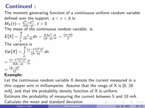
Continued :The moment generating function of a continuous uniform random variabledefined over the support. a < x < b is:MX (t) = ebt−eat

t(b−a) , t > 0The mean of the continuous random variable. is

E [X ] =b∫a

x(b−a)dx = 0.5x2

(b−a) |ba . = (a+b)

2

The variance is

Var [X ] =b∫a

(x−( a+b2

))2

(b−a) dx

=(x−( a+b

2))3

3(b−a) |ba

= (b−a)2

12Example:Let the continuous random variable X denote the current measured in athin copper wire in milliamperes. Assume that the range of X is [0, 20mA], and that the probability density function of X is uniform.Estimate the probability of measuring the current between 5 and 10 mA.Calculate the mean and standard deviation.


Exponential Random Variable :A continuous random variable X is said to have an exponential distributionwith parameter λ > 0, if its PDF is given by

f (x) =

{λe−λx , x > 0

0, otherwise

Figure: A schematic of pdf and cdf of exponential continuous distribution

The CDF of the exponential variable is given byF (x) = P(X ≤ x)

=x∫0

λe−λtdt

= 1 - e−λx , x ≥ 0Sadhana Dash Basic Statistics July 16, 2021 40 / 72

Normal Random Variable

A random variable X is normal random variable if the pdf is given by

f (x) = 1√2πσ

e−(x−µ)2

2σ2 , −∞ < x <∞with parameters µ ( −∞ < µ <∞) and σ > 0.

Figure: A schematic of pdf and cdf of normal continuous distribution


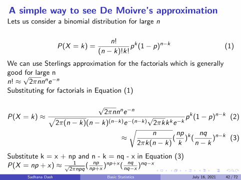
A simple way to see De Moivre’s approximationLets us consider a binomial distribution for large n

P(X = k) =n!

(n − k)!k!pk(1− p)n−k (1)

We can use Sterlings approximation for the factorials which is generallygood for large nn! ≈

√2πnnne−n

Substituting for factorials in Equation (1)

P(X = k) ≈√

2πnnne−n√2π(n − k)(n − k)(n−k)e−(n−k)

√2πkkke−k

pk(1− p)n−k (2)

≈√

n

2πk(n − k)(np

k)k(

nq

n − k)n−k (3)

Substitute k = x + np and n - k = nq - x in Equation (3)P(X = np + x) ≈ 1√

2πnpq( npnp+x )np+x( nq

nq−x )nq−x


Continued :

P(X = np + x) ≈ 1√2πnpq

(np

np + x)np+x(

nq

nq − x)nq−x (4)

≈ C (np + x

np)−np−x(

nq − x

nq)−nq+x (5)

≈ C (1 +x

np)−np−x(1− x

nq)−nq+x (6)

We can take logarithm of both the sides

lnP(X = np + x) ≈ lnC − (np + x)ln(1 +x

np)− (nq − x)ln(1− x

nq) (7)

We can useln(1 + x) = x − 1

2x2 + 1

3x3 − · · · (−1)n 1

nxn

ln(1− x) = −x − 12x

2 − 13x

3 − · · · − 1nx

n


Continued :

Keeping only the first two terms of the expansion in Equation (7)

≈ lnC − (np + x)(x

np− x2

2(np)2)− (nq − x)(− x

nq− x2

2(nq)2) (8)

≈ lnC − x − x2

np+

x2

2np+

x3

2(np)3+ x − x2

nq+

x2

2nq− x3

2(nq)3(9)

≈ lnC − x2

2npq(10)

P(X = k) ≈ 1√2πnpq

exp(−12

(k−np)2

npq ) (11)

One can notice, for a binomial distribution, µ = np and σ2 = npq

P(X = k) ≈ 1σ√

2πexp(−1

2(k−µ)2

σ2 )


Properties of a normal random variable

f (x) > 0 for all x∞∫−∞

f (x) = 1

∞∫−∞

f (x) =∞∫−∞

1√2πσ

e−(x−µ)2

2σ2 dx

Substituting x−µσ = z , dx =σ dz

I =∞∫−∞

1√2πe−

12z2dz

Squaring both the sides

I2 = [∞∫−∞

1√2πe−

12x2dx ][

∞∫−∞

1√2πe−

12y2dy ]

= 12π

∞∫−∞

∞∫−∞

e−12

(x2+y2)dxdy


continued

I 2 = 12π

∞∫−∞

∞∫−∞

e−12

(x2+y2)dxdy

Let us do a change of variable in polar coordinates ; x = rcosθ , y = rsinθ

I2 = 12π

2π∫0

(∞∫0

e−r2

2 rdrdθ)

let u = r2/2, du = rdr

I2 = 12π

2π∫0

(∞∫0

e−udu)dθ

= 12π

2π∫0

−(0− 1)dθ = 1

I = ±1But f (x) > 0, I = +1.


continued

All normal random variables are symmetric about µ.f (µ+ x) = f (µ− x)

f (µ+ x) = 1√2πσ

e−(x+µ−µ)2

2σ2

= 1√2πσ

e−x2

2σ2

f (µ− x) = 1√2πσ

e−(µ−x−µ)2

2σ2

= 1√2πσ

e−x2

2σ2

The point of inflection of a normal distribution is µ± σ


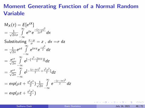
Moment Generating Function of a Normal RandomVariable

MX (t) = E [etX ]

= 1√2πσ

∞∫−∞

etxe−(x−µ)2

2σ2 dx

Substituting x−µσ = z , dx =σ dz

= 1√2πeµt

∞∫−∞

etσze−z2

2 dz

= eµt√2π

∞∫−∞

e [−( z2−2tσz2

)]dz

= eµt√2π

∞∫−∞

e [− (z−tσ)2

2+ t2σ2

2]dz

= exp(µt + t2σ2

2 ) 1√2π

∞∫−∞

e−(z−tσ)2

2 dz

= exp(µt + t2σ2

2 )


Mean and Variance

MX (t) = exp(µt +t2σ2

2) (12)

Differentiating w.r.t t

M′X (t) = (µ+ tσ2)exp(µt +

t2σ2

2) (13)

M′′X (t) = σ2exp(µt +

t2σ2

2) + (µ+ tσ2)2exp(µt +

t2σ2

2) (14)

E [X ] = M′X (0) = µ

E [X 2] = M′′X (0) = σ2 + µ2

Var [X ] = E [X 2]− (E [X ])2 = σ2


For a normal distribution one can show thatapproximately 68% of the data fall within one standard deviation of themeanapproximately 95% of the data fall within two standard deviations of themeanapproximately 99.7% of the data fall within three standard deviations ofthe mean


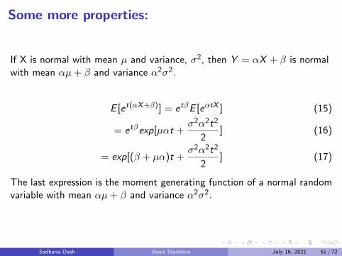
Some more properties:

If X is normal with mean µ and variance, σ2, then Y = αX + β is normalwith mean αµ+ β and variance α2σ2.

E [et(αX+β)] = etβE [eαtX ] (15)

= etβexp[µαt +σ2α2t2

2] (16)

= exp[(β + µα)t +σ2α2t2

2] (17)

The last expression is the moment generating function of a normal randomvariable with mean αµ+ β and variance α2σ2.


The sum of independent normal random variables is also a normal random

variable with mean µ =n∑

i=1µi and σ2 =

n∑i=1

σ2i

Let Xi , i = 1, · · · , n, are independent normal random variables withmean, µi and variance, σ2

i .

The moment generating function ofn∑

i=1Xi is

E [e(t

n∑i=1

Xi )] = E [etX1 · · · eXn ] (18)

=n∏

i=1

E [etXi ] =n∏

i=1

eµi t+(σ2i t

2)/2 = eµt+(σ2t2)/2 (19)

where µ =n∑iµi and σ2 =

n∑iσ2i


Standard Normal Random Variable

A normal random variable with µ = 0 and σ2 = 1 is called a standardnormal random variable and is denoted by Z ∼ N(0, 1)

fZ (z) = 1√2πe−z2

2 , −∞ < z <∞The cumulative distribution function of a standard normal random variableis denoted as Φ(x) is

Φ(x) = P(Z ≤ x) = 1√2π

x∫−∞

e−t2

2dt

Properties

limx→∞

Φ(x) = 1

limx→−∞

Φ(x) = 0

Φ(0) = 1/2

Φ(−x) = 1− Φ(x)


We can obtain any normal random variable by shifting and scaling astandard normal random variable.X = σZ + µ, σ > 0E [X ] = σE [Z ] + µ = µVar [X ] = σ2Var(Z ) = σ2

.If Z is a standard normal random variable and X = σZ + µ, then X is anormal random variable with mean µ and variance σ2i .e,X ∼ N(µ, σ2)

If X ∼ N(µ, σ2), the random variable defined by Z = (X−µ)σ is a standard

normal random variable, i.e., Z ∼ N(0, 1).

FX (x) = P(X ≤ x) = P(σZ + µ ≤ x)(20)

= P(Z ≤ (x − µ)

σ) (21)

= Φ(x − µσ

) (22)


For any a < b

P(a < X < b) = P((a− µ)

σ<

(X − µ)

σ<

(b − µ)

σ) (23)

= P((a− µ)

σ< Z <

(b − µ)

σ) (24)

= P(Z <(b − µ)

σ)− P(Z <

(a− µ)

σ) (25)

P(a < X < b) = Φ(b − µσ

)− Φ(a− µσ

) (26)



Example :If X ∼ N(−5, 4)Find P(X < 0)Find P(−7 < X < −3)Find P(X > −3|X > −5)SolutionX is a random variable with mean -5 and σ = 2(1) P(X < 0) = F (0) = Φ( 0−(−5)

2 ) = Φ(2.5)

(2) P(−7 < X < −3) = Φ(−3−(−5)2 )− Φ(−7−(−5)

2 )= Φ(1)− Φ(−1) = 2Φ(1)− 1

(3) P(X > −3|X > −5) = P(X>−3,X>−5)P(X>−5)

= P(X>−3)P(X>−5)

= 1−Φ(1)1−Φ(0)


Example :

Let the background noise follows a normal distribution with a mean of 0volt and standard deviation of 0.4 volt in the detection of a digital signal.The system assumes that a digital 1 has been transmitted when thevoltage exceeds 0.8. What is the probability of detecting a digital 1 whennone was sent?Solution:Let X denote the random variable which denote the voltage of noise.P(X > 0.8) = P(X−0

0.4 > 0.8/0.4) = P(Z > 2) = 1− Φ(2) = 0.022


The Chi-Square Distribution:

If Z1, Z2, ... , Zn are independent standard normal random variables, therandom variable Y defined asY= Z 2

1 +Z 22 + · · ·+Z2

n

is said to have a chi-square (χ2n) distribution with n degrees of freedom

shown by Y ∼ χ2n

Figure: Schematic of χ2n distribution for different degrees of freedom.


Properties:If Y1 and Y2 are independent chi-square random variables with n1 and n2

degrees of freedom, respectively, then Y1 + Y2 is a chi-square randomvariable with n1 + n2 degrees of freedom.If X is a chi-square random variable with n degrees of freedom, then forany α ∈ (0, 1) the quantity χ2

α,n is defined to be such thatP(X ≥ χ2

α,n) = α


The Moment Generating Function:

The moment generating function of a chi-square random variable with ndegrees of freedom isMX (t) = E [etX ] = E [etZ

2] where Z ∼ N(0,1)

= 1√2π

∞∫−∞

etx2e−x2

2 dx = 1√2π

∞∫−∞

e−x2(1−2t)

2 dx

if σ2 = (1− 2t)−1

= 1√2π

∞∫−∞

e−x2

2σ2 dx = (1− 2t)−1/2 1√2πσ2

∞∫−∞

e−x2

2σ2 dx

= (1− 2t)−1/2

When X =n∑

i=1Z 2i

E[etX ] = (1− 2t)−n/2

E[X] = nVar[X] = 2n


Central moments

Central moments are moments about the mean, µµn = E[(X - µ)n]Raw momentsµ′n = E[(X)n]

First central moment = µ1 = 0Second central moment = µ2 = σ2 = µ

′2 − µ2

Third central moment = µ3 = µ′3 − 3µ

′1µ′2 + 2µ3

Fourth central moment = µ4 = µ′4 − 4µµ

′3 + 6µ2µ

′2 − 3µ4

The standardized moment of degree n is

standardized moment =µnσn

(27)

where σ is the standard deviation.


Skewness

The term skewness is a measure of lack of symmetry or departure fromsymmetry of the probability distribution function. If the distribution is notsymmetrical (or is asymmetrical) about the mean, it is called a skeweddistribution.If the bulk of the data is at the left and the right tail is longer, thedistribution is skewed right or positively skewed.If the bulk of the data is towards the right and the left tail is longer, wesay that the distribution is skewed left or negatively skewed.


Measure of Skewness

The skewness is quantified as the third standardized moment.

β1 =µ2

3

µ32

Pearson’s coefficient of skewnessγ1 =

√β1

Estimate the skewness of normal and exponential distribution.


Kurtosis

Kurtosis refers to the height and sharpness of the peak relative to anormal distribution. Sometimes, it is also interpreted as the tailedness ofthe pdf. Higher values indicate a higher, sharper peak; lower valuesindicate a lower, less distinct peak.The reference standard is a normal distribution, which has a kurtosis of 3.Therefore, excess kurtosis is defined as kurtosis - 3.A normal distribution has kurtosis exactly 3 (excess kurtosis =0).Any distribution with kurtosis = 3 (excess kurtosis = 0) is calledmesokurtic.A distribution with kurtosis < 3 (excess kurtosis < 0) is called platykurtic.A distribution with kurtosis > 3 (excess kurtosis > 0) is called leptokurtic.


Measure of Kurtosis

β2 = µ4

µ22

Excess Kurtosisγ2 = β2 − 3

Estimate the kurtosis of a normal distribution


Summarizing Data Sets

Sample Mean :The sample mean characterizes the central tendency in the data by thearithmetic average.Let us consider a sample of size n with numerical values, x1, x2, x3...xn.The arithmetic average of the values is called sample mean.

x =

n∑i=1

xi

n(28)

ExampleLets consider the eight observations , 13.8, 14.9, 13.4, 15.3, 13.6, 13.5,12.6, and 13.1 which constitutes a sample . Calculate the sample mean.


If a data set is presented in a frequency table where the k distinct values,v1, ..., vk , having corresponding frequencies f1, ..., fk such that n =

∑ki=1 fi ,

the sample mean of these n data values is

x =

k∑i=1

vifi

n(29)

Therefore, the sample mean is a weighted average of the distinct values,where the weight given to the value vi is equal to the proportion of the ndata values that are equal to vi , i = 1, . . . , k.


Sample median

Sample median is the middle value when the data set is arranged inincreasing order.Determination of median :Order the values of a data set of size n from smallest to largest.If n is odd, the sample median is the value in position (n + 1)/2if n is even, it is the average of the values in positions n/2 and n/2 + 1.Sample modeThe value that occurs with the greatest frequency.


Sample Variance

This statistic describes the variability or scatter in the data.The sample variance , s2 (of a data set x1, x2, x3...xn ) is given by,

s2 =

n∑i=1

(xi − x)2

(n− 1)(30)

The sample standard deviation is given by

s =

√√√√√ n∑i=1

(xi − x)2

(n− 1)(31)

Show thatn∑

i=1(xi − x)2 = (

n∑i=1

x2i )− nx2 Note: While calculating variance for

population, one divides by N, size of population .


Sample Correlation CoefficientIf sx and sy denote, respectively, the sample standard deviations of the xvalues and the y values in a paired data set, the sample correlationcoefficient, r , of the data pairs (xi , yi ) , i = 1, . . . , n is defined by

r =

n∑i=1

(xi − x)(yi − y)

(n− 1)sxsy(32)

When r > 0 , the sample data pairs are positively correlated, and whenr < 0 , they are negatively correlated.Properties of r

1 −1 ≤ r ≤ 12 if yi = a + bxi , for i = 1,2,.. n then r = 1 (for b > 0) and r = −1

(for b < 0) where a and b are constants.3 If r is the sample correlation coefficient for the data pairs (xi , yi ) , i=

1,..., n then it is also the sample correlation coefficient for the datapairs a + bxi , c + dyi , i=1,...,n provided that b and d are bothpositive or both negative constants.


Sample Correlation Coefficient

Figure:Sadhana Dash Basic Statistics July 16, 2021 72 / 72

Documents

Basic Statistics - CERN Indico