Embed Size (px)
Citation preview
Timing and Synchronization
Marco Bellaveglia [email protected]
Timing and Synchronization CAS– FEL & ERL – Hamburg, Germany 1
Lecture outline
1. General overview
2. Introduction to phase noise
3. Synchronization in linear injectors
4. Timing in linear injectors
5. References
Timing and Synchronization 2 CAS– FEL & ERL – Hamburg, Germany
Timing and Synchronization 3
1. General overview
CAS– FEL & ERL – Hamburg, Germany
1. Definitions
2. Synchronization
3. Timing
1.1. General Overview - Definitions
• Synchronization: A fine temporal alignment among all the relevant sub-system oscillators that guarantees temporal coherence of their outputs (precision 10ps÷10fs) – Example: coherence between RF accelerating phase
– laser oscillators frequency – ADC/DAC clocks
• Timing: digital delayed signals that define the temporization of events (precision 10ns÷10ps) – Example: RF pulse generation, lasers amplification
temporal gate, BPM triggers, injection/extraction kickers, event tagging, …
Timing and Synchronization 4 CAS– FEL & ERL – Hamburg, Germany
1.2. General overview - Synchronization
Timing and Synchronization 5
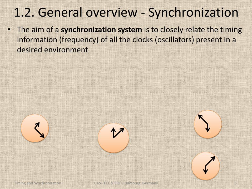
• The aim of a synchronization system is to closely relate the timing information (frequency) of all the clocks (oscillators) present in a desired environment
CAS– FEL & ERL – Hamburg, Germany
1.2. General overview - Synchronization
Timing and Synchronization 6
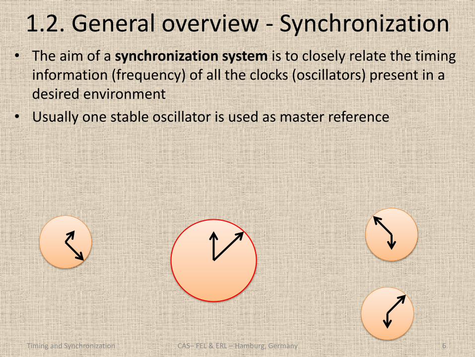
• The aim of a synchronization system is to closely relate the timing information (frequency) of all the clocks (oscillators) present in a desired environment
• Usually one stable oscillator is used as master reference
CAS– FEL & ERL – Hamburg, Germany
1.2. General overview - Synchronization
Timing and Synchronization 7
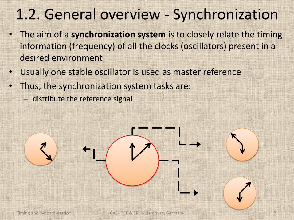
• The aim of a synchronization system is to closely relate the timing information (frequency) of all the clocks (oscillators) present in a desired environment
• Usually one stable oscillator is used as master reference
• Thus, the synchronization system tasks are: – distribute the reference signal
CAS– FEL & ERL – Hamburg, Germany
1.2. General overview - Synchronization
Timing and Synchronization 8
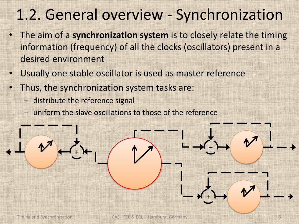
• The aim of a synchronization system is to closely relate the timing information (frequency) of all the clocks (oscillators) present in a desired environment
• Usually one stable oscillator is used as master reference
• Thus, the synchronization system tasks are: – distribute the reference signal
– uniform the slave oscillations to those of the reference
+
+
+
CAS– FEL & ERL – Hamburg, Germany
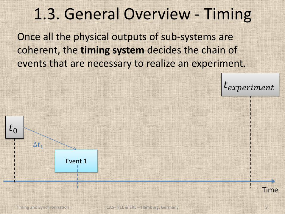
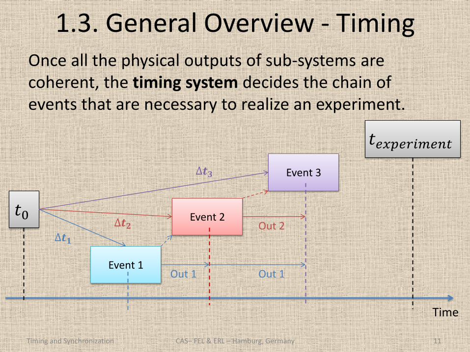
1.3. General Overview - Timing Once all the physical outputs of sub-systems are coherent, the timing system decides the chain of events that are necessary to realize an experiment.
Timing and Synchronization 9
Event 1
Time
𝑡0
∆𝒕𝟏
𝑡𝑒𝑥𝑝𝑒𝑟𝑖𝑚𝑒𝑛𝑡
CAS– FEL & ERL – Hamburg, Germany
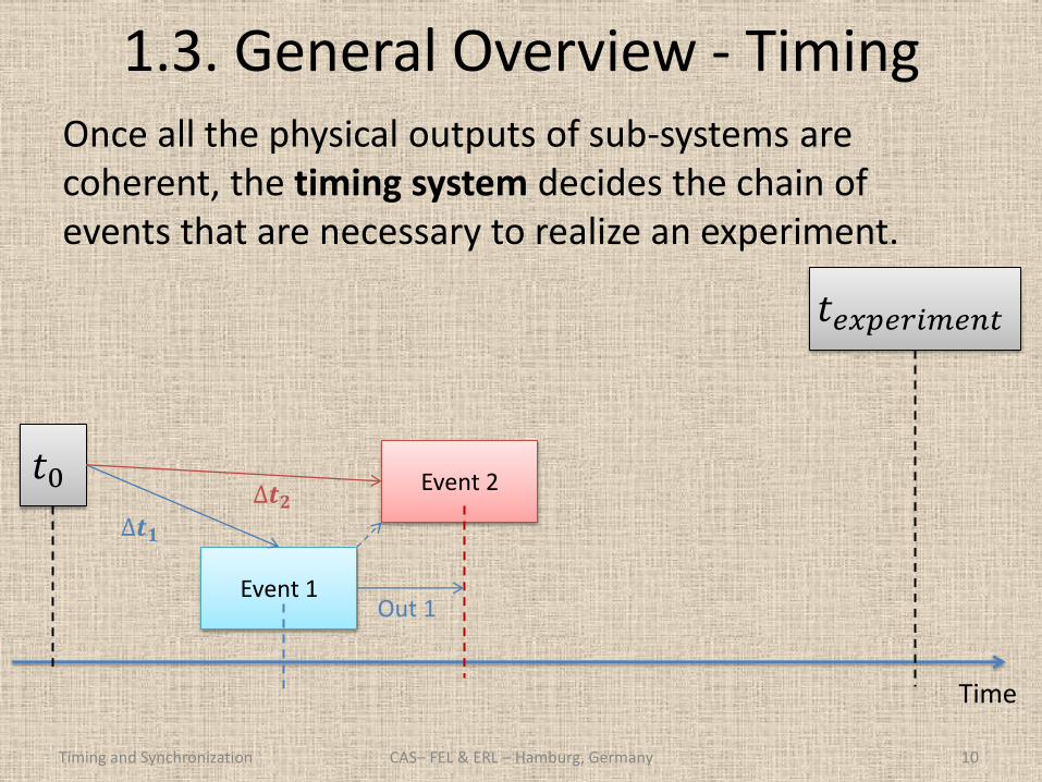
1.3. General Overview - Timing Once all the physical outputs of sub-systems are coherent, the timing system decides the chain of events that are necessary to realize an experiment.
Timing and Synchronization 10
Event 1
Time
Event 2 𝑡0
∆𝒕𝟏
∆𝒕𝟐
Out 1
𝑡𝑒𝑥𝑝𝑒𝑟𝑖𝑚𝑒𝑛𝑡
CAS– FEL & ERL – Hamburg, Germany
1.3. General Overview - Timing Once all the physical outputs of sub-systems are coherent, the timing system decides the chain of events that are necessary to realize an experiment.
Timing and Synchronization 11
Event 1
Time
Event 2
Event 3
𝑡0
∆𝒕𝟏
∆𝒕𝟐
∆𝒕𝟑
Out 1
Out 2
Out 1
𝑡𝑒𝑥𝑝𝑒𝑟𝑖𝑚𝑒𝑛𝑡
CAS– FEL & ERL – Hamburg, Germany
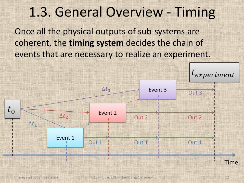
1.3. General Overview - Timing
Timing and Synchronization 12
Event 1
Time
Event 2
Event 3
𝑡0
∆𝒕𝟏
∆𝒕𝟐
∆𝒕𝟑
Out 1
Out 2
Out 1
𝑡𝑒𝑥𝑝𝑒𝑟𝑖𝑚𝑒𝑛𝑡
Out 1
Out 2
Out 3
CAS– FEL & ERL – Hamburg, Germany
Once all the physical outputs of sub-systems are coherent, the timing system decides the chain of events that are necessary to realize an experiment.
Timing and Synchronization 13
2. Introduction to phase noise
CAS– FEL & ERL – Hamburg, Germany
1. Phase noise in oscillators
2. Noise sources
3. Measuring phase noise
Timing and Synchronization 14
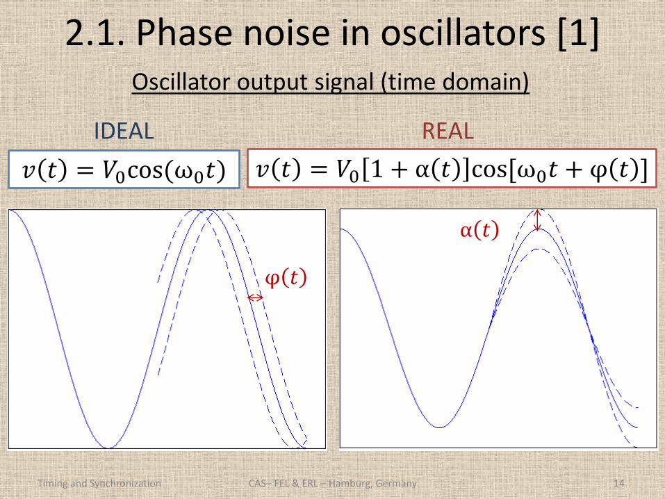
2.1. Phase noise in oscillators [1]
𝑣 𝑡 = 𝑉0 1 + α 𝑡 cos[ω0𝑡 + φ 𝑡 ]
φ 𝑡
α 𝑡
Oscillator output signal (time domain)
𝑣 𝑡 = 𝑉0cos(ω0𝑡)
IDEAL REAL
CAS– FEL & ERL – Hamburg, Germany
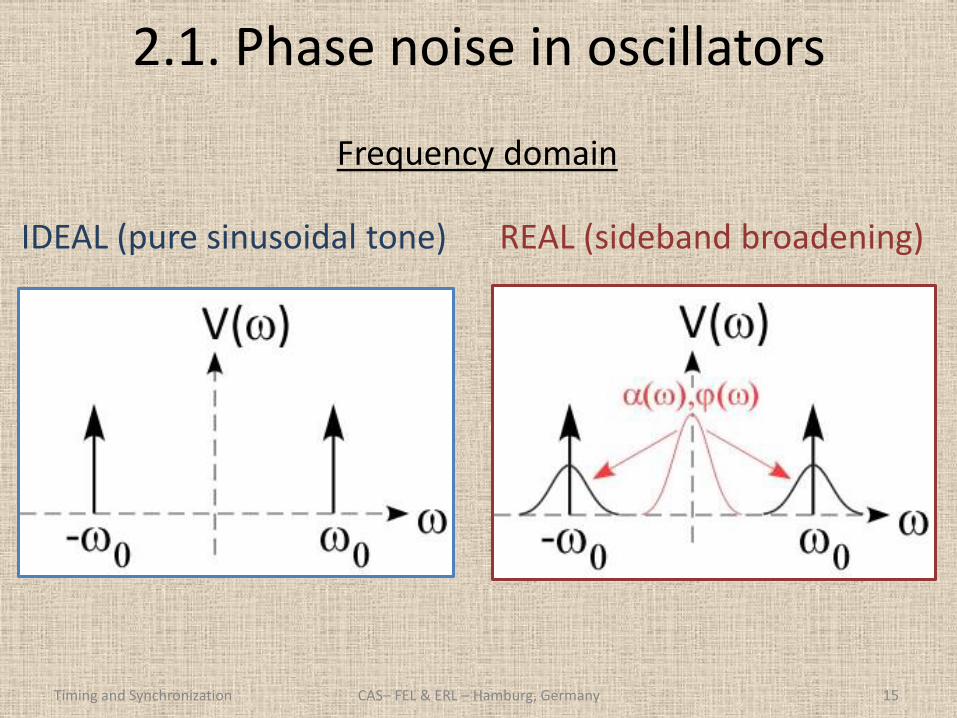
2.1. Phase noise in oscillators
Timing and Synchronization 15
Frequency domain
IDEAL (pure sinusoidal tone) REAL (sideband broadening)
CAS– FEL & ERL – Hamburg, Germany
2.1. Phase noise in oscillators
Timing and Synchronization 16
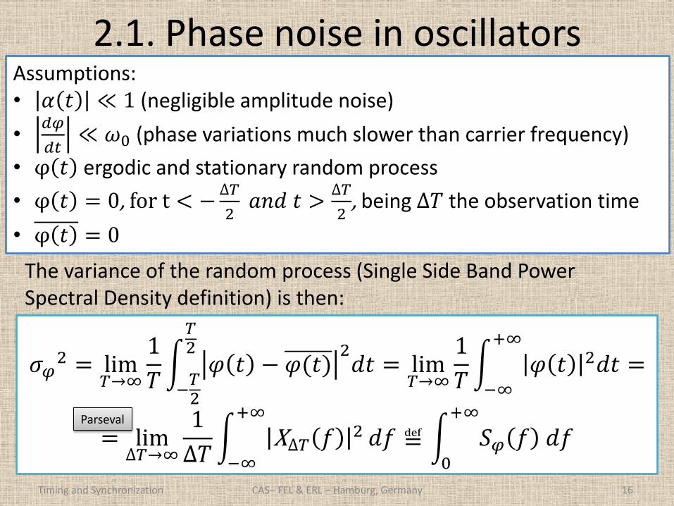
The variance of the random process (Single Side Band Power Spectral Density definition) is then:
𝜎𝜑2 = lim
𝑇→∞
1
𝑇 𝜑 𝑡 − 𝜑(𝑡)
2𝑑𝑡
𝑇2
−𝑇2
= lim𝑇→∞
1
𝑇 𝜑 𝑡 2𝑑𝑡
+∞
−∞
=
= lim∆𝑇→∞
1
∆𝑇 X∆𝑇 𝑓 2
+∞
−∞
𝑑𝑓 ≝ 𝑆𝜑 𝑓 𝑑𝑓+∞
0
Assumptions: • 𝛼 𝑡 ≪ 1 (negligible amplitude noise)
•𝑑𝜑
𝑑𝑡≪ 𝜔0 (phase variations much slower than carrier frequency)
• φ 𝑡 ergodic and stationary random process
• φ 𝑡 = 0, for t < −∆𝑇
2𝑎𝑛𝑑𝑡 >
∆𝑇
2, being ∆𝑇 the observation time
• φ 𝑡 = 0
Parseval
CAS– FEL & ERL – Hamburg, Germany
2.1. Phase noise in oscillators
Timing and Synchronization 17
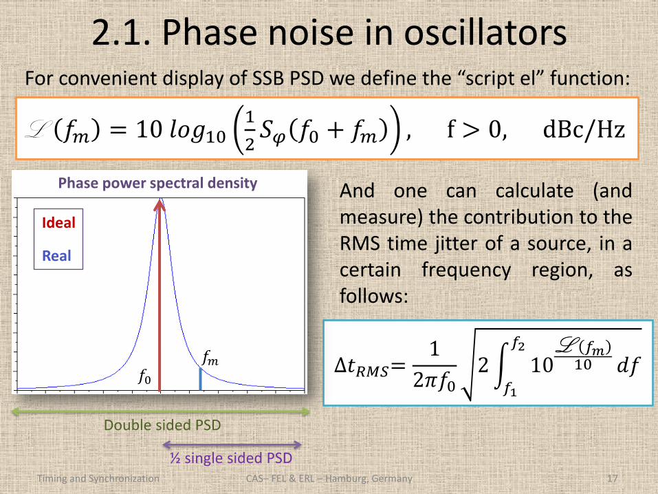
L 𝑓𝑚 = 10𝑙𝑜𝑔101
2𝑆𝜑 𝑓0 + 𝑓𝑚 , f > 0, dBc/Hz
For convenient display of SSB PSD we define the “script el” function:
∆𝑡𝑅𝑀𝑆=1
2𝜋𝑓02 10
L 𝑓𝑚10
𝑓2
𝑓1
𝑑𝑓
Ideal
Real
Phase power spectral density
𝑓0 𝑓𝑚
½ single sided PSD
Double sided PSD
And one can calculate (and measure) the contribution to the RMS time jitter of a source, in a certain frequency region, as follows:
CAS– FEL & ERL – Hamburg, Germany
2.2. Noise sources
Timing and Synchronization 18
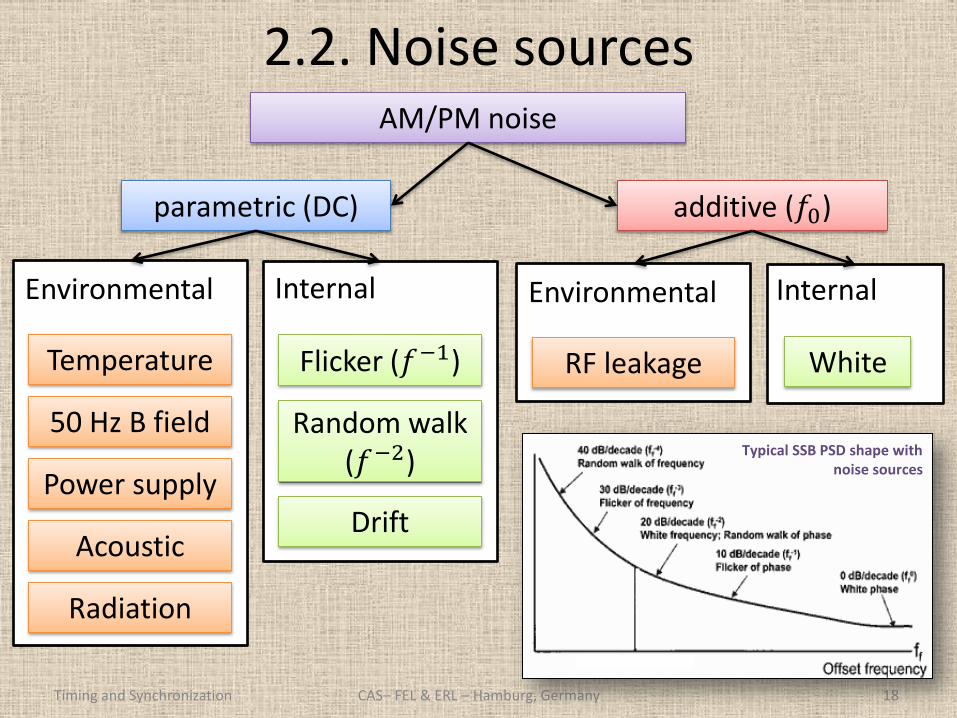
AM/PM noise
parametric (DC) additive (𝑓0)
Environmental
Temperature
50 Hz B field
Power supply
Acoustic
Radiation
Internal
Flicker (𝑓−1)
Random walk (𝑓−2)
Drift
Environmental
RF leakage
Internal
White
CAS– FEL & ERL – Hamburg, Germany
Typical SSB PSD shape with noise sources
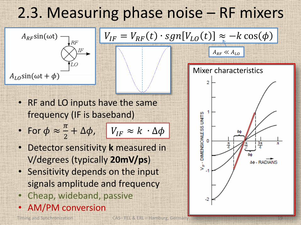
2.3. Measuring phase noise – RF mixers
Timing and Synchronization 19
Mixer characteristics
• RF and LO inputs have the same frequency (IF is baseband)
• For 𝜙 ≈𝜋
2+ ∆𝜙,
• Detector sensitivity k measured in V/degrees (typically 20mV/ps)
• Sensitivity depends on the input signals amplitude and frequency
• Cheap, wideband, passive • AM/PM conversion
𝑉𝐼𝐹 = 𝑉𝑅𝐹 𝑡 ∙ 𝑠𝑔𝑛 𝑉𝐿𝑂 𝑡 ≈ −𝑘 cos 𝜙
𝑉𝐼𝐹 ≈ 𝑘 ∙ ∆𝜙
CAS– FEL & ERL – Hamburg, Germany
𝐴𝑅𝐹sin(ωt)
𝐴𝐿𝑂sin(ωt + 𝜙)
𝐴𝑅𝐹 ≪ 𝐴𝐿𝑂
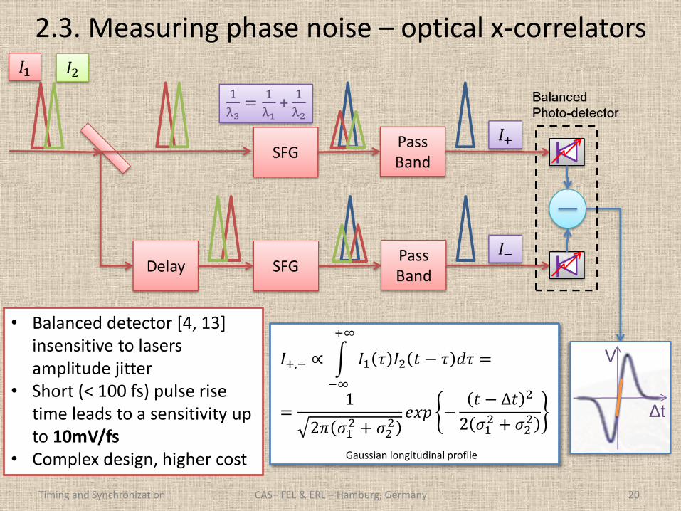
2.3. Measuring phase noise – optical x-correlators
Timing and Synchronization 20
• Balanced detector [4, 13] insensitive to lasers amplitude jitter
• Short (< 100 fs) pulse rise time leads to a sensitivity up to 10mV/fs
• Complex design, higher cost
CAS– FEL & ERL – Hamburg, Germany
𝐼+,− ∝ 𝐼1 𝜏 𝐼2 𝑡 − 𝜏 𝑑𝜏
+∞
−∞
=
=1
2𝜋 𝜎12 + 𝜎2
2𝑒𝑥𝑝 −
𝑡 − ∆𝑡 2
2 𝜎12 + 𝜎2
2
Gaussian longitudinal profile
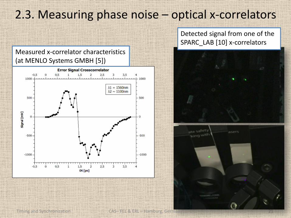
2.3. Measuring phase noise – optical x-correlators
Timing and Synchronization 21
Measured x-correlator characteristics (at MENLO Systems GMBH [5])
Detected signal from one of the SPARC_LAB [10] x-correlators
CAS– FEL & ERL – Hamburg, Germany
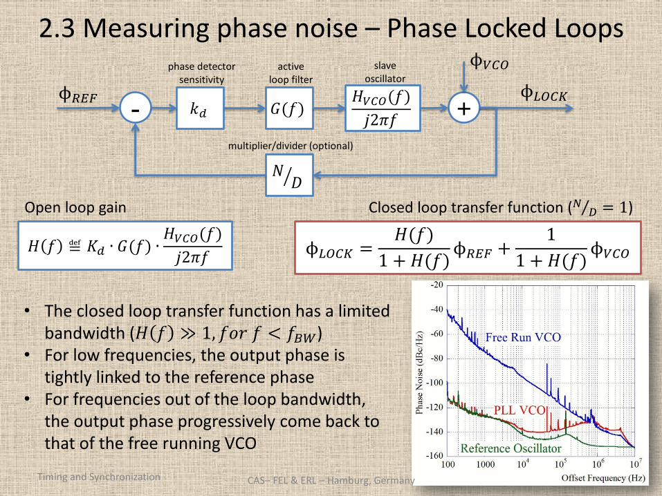
2.3 Measuring phase noise – Phase Locked Loops
Timing and Synchronization 22
ϕ𝑅𝐸𝐹 𝑘𝑑 𝐺(𝑓)
𝐻𝑉𝐶𝑂(𝑓)
𝑗2𝜋𝑓 - +
ϕ𝐿𝑂𝐶𝐾
ϕ𝐿𝑂𝐶𝐾 =𝐻(𝑓)
1 + 𝐻(𝑓)ϕ𝑅𝐸𝐹 +
1
1 + 𝐻(𝑓)ϕ𝑉𝐶𝑂 𝐻 𝑓 ≝ 𝐾𝑑 ∙ 𝐺(𝑓) ∙
𝐻𝑉𝐶𝑂(𝑓)
𝑗2𝜋𝑓
Open loop gain Closed loop transfer function (𝑁 𝐷 = 1)
• The closed loop transfer function has a limited bandwidth (𝐻 𝑓 ≫ 1, 𝑓𝑜𝑟𝑓 < 𝑓𝐵𝑊)
• For low frequencies, the output phase is tightly linked to the reference phase
• For frequencies out of the loop bandwidth, the output phase progressively come back to that of the free running VCO
phase detector sensitivity
active loop filter
slave oscillator
𝑁𝐷
multiplier/divider (optional)
ϕ𝑉𝐶𝑂
CAS– FEL & ERL – Hamburg, Germany
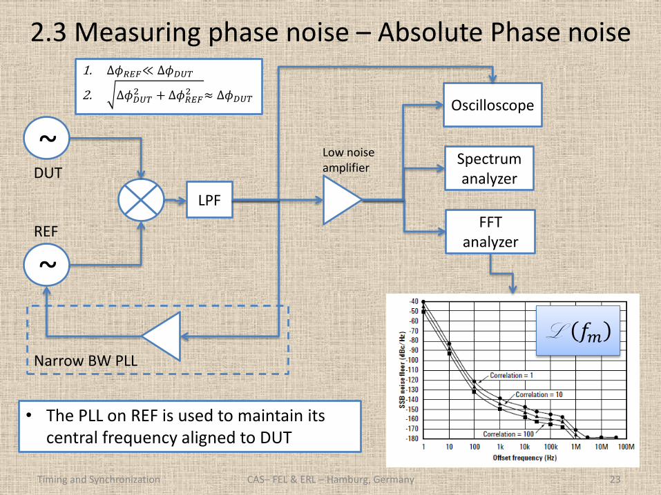
2.3 Measuring phase noise – Absolute Phase noise
Timing and Synchronization 23
• The PLL on REF is used to maintain its central frequency aligned to DUT
CAS– FEL & ERL – Hamburg, Germany
L 𝑓𝑚
DUT
REF
~
~
LPF
Narrow BW PLL
Low noise amplifier
Spectrum analyzer
FFT analyzer
Oscilloscope
1. ∆𝜙𝑅𝐸𝐹≪ ∆𝜙𝐷𝑈𝑇
2. ∆𝜙𝐷𝑈𝑇2 + ∆𝜙𝑅𝐸𝐹
2 ≈ ∆𝜙𝐷𝑈𝑇
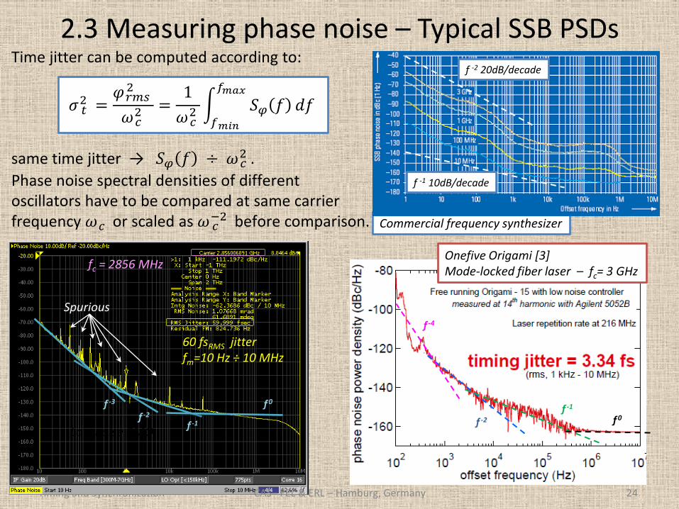
2.3 Measuring phase noise – Typical SSB PSDs
Timing and Synchronization 24
Time jitter can be computed according to:
same time jitter → 𝑆𝜑 𝑓 ÷ 𝜔 𝑐2 .
Phase noise spectral densities of different oscillators have to be compared at same carrier frequency 𝜔 𝑐 or scaled as 𝜔 𝑐
−2 before comparison.
𝜎 𝑡2 =
𝜑 𝑟𝑚𝑠2
𝜔 𝑐2 =
1
𝜔 𝑐2 𝑆𝜑 𝑓
𝑓𝑚𝑎𝑥
𝑓𝑚𝑖𝑛
𝑑𝑓
60 fsRMS jitter fm=10 Hz ÷ 10 MHz
fc = 2856 MHz
f -1
f -2
f -3
Spurious
f -1
f -2
f -4
Commercial frequency synthesizer
Low noise RMO
Onefive Origami [3] Mode-locked fiber laser – fc= 3 GHz
f 0
f 0
f -2 20dB/decade
f -1 10dB/decade
CAS– FEL & ERL – Hamburg, Germany
Timing and Synchronization 25
3. Synchronization in linear injectors
CAS– FEL & ERL – Hamburg, Germany
1. Experiment requirements
2. Overview
3. Reference generation
4. Reference distribution
5. Client locking
6. Beam timing jitter
7. Diagnostics
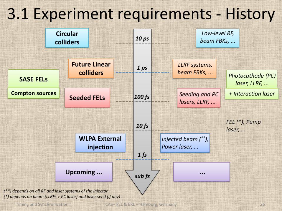
3.1 Experiment requirements - History
Timing and Synchronization 26
10 ps
1 ps
100 fs
10 fs
1 fs
sub fs
Circular colliders
Low-level RF, beam FBKs, ...
Future Linear colliders
LLRF systems, beam FBKs, ...
SASE FELs Photocathode (PC)
laser, LLRF, ...
Seeded FELs
WLPA External injection
Upcoming ...
Seeding and PC lasers, LLRF, ...
FEL (*), Pump laser, ...
Injected beam (**), Power laser, ...
...
+ Interaction laser Compton sources
(**) depends on all RF and laser systems of the injector (*) depends on beam (LLRFs + PC laser) and laser seed (if any)
CAS– FEL & ERL – Hamburg, Germany
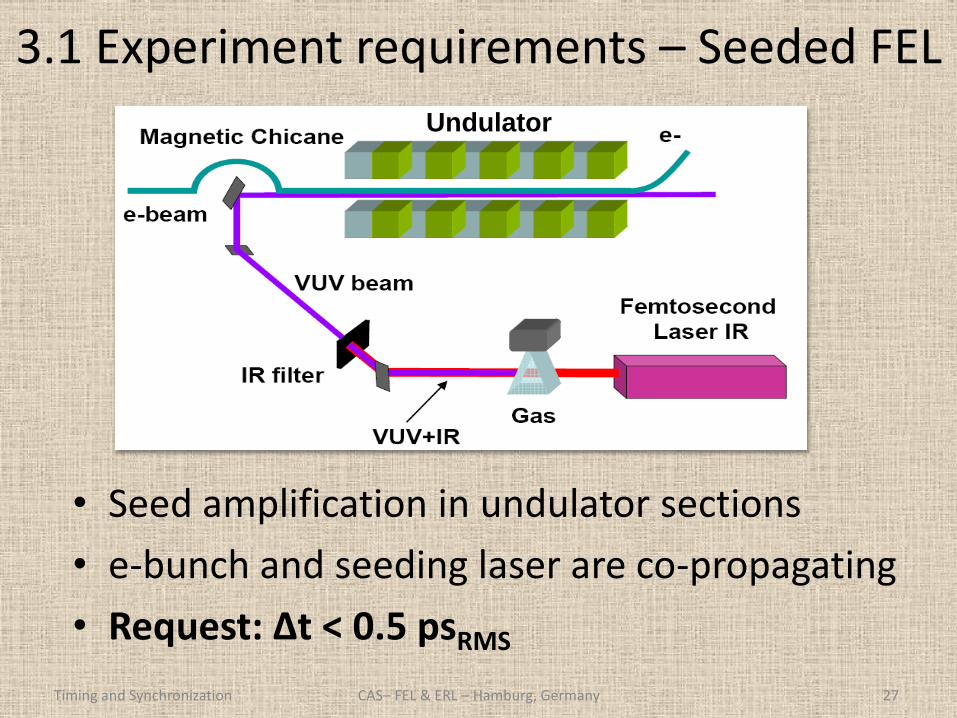
3.1 Experiment requirements – Seeded FEL
Timing and Synchronization 27
• Seed amplification in undulator sections
• e-bunch and seeding laser are co-propagating
• Request: Δt < 0.5 psRMS
Undulator
CAS– FEL & ERL – Hamburg, Germany
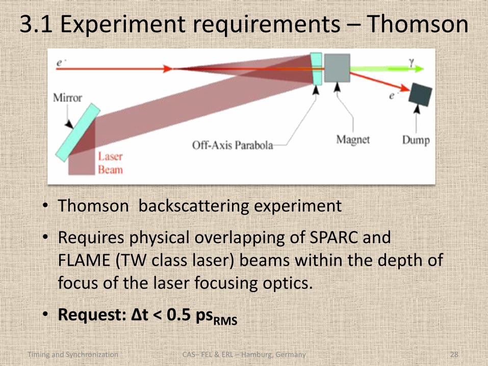
3.1 Experiment requirements – Thomson
Timing and Synchronization 28
• Thomson backscattering experiment
• Requires physical overlapping of SPARC and FLAME (TW class laser) beams within the depth of focus of the laser focusing optics.
• Request: Δt < 0.5 psRMS
CAS– FEL & ERL – Hamburg, Germany
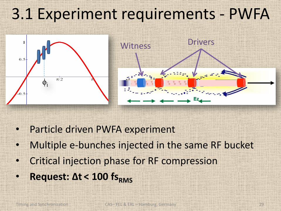
3.1 Experiment requirements - PWFA
Timing and Synchronization 29
• Particle driven PWFA experiment
• Multiple e-bunches injected in the same RF bucket
• Critical injection phase for RF compression
• Request: Δt < 100 fsRMS
Drivers Witness
CAS– FEL & ERL – Hamburg, Germany
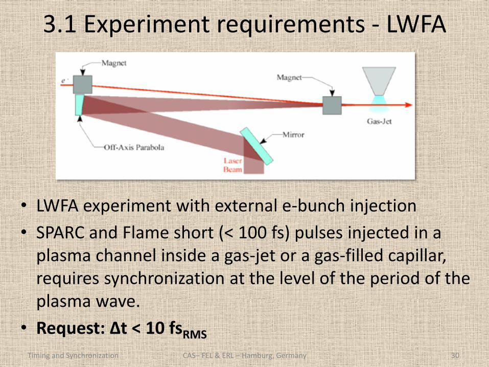
3.1 Experiment requirements - LWFA
Timing and Synchronization 30
• LWFA experiment with external e-bunch injection
• SPARC and Flame short (< 100 fs) pulses injected in a plasma channel inside a gas-jet or a gas-filled capillar, requires synchronization at the level of the period of the plasma wave.
• Request: Δt < 10 fsRMS
CAS– FEL & ERL – Hamburg, Germany
3.2 Overview – General concepts
Timing and Synchronization 31
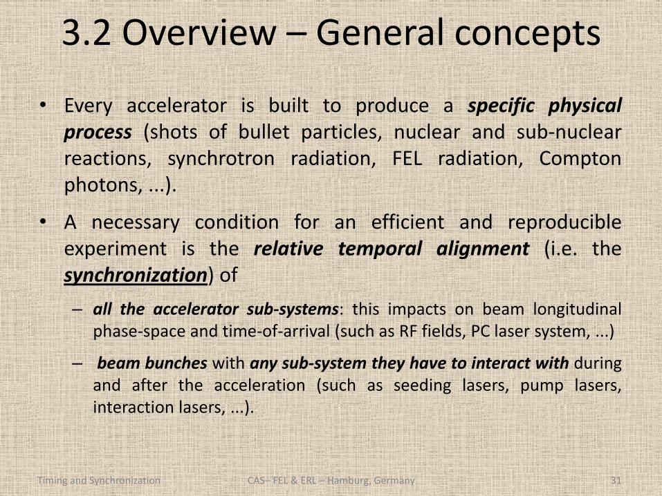
• Every accelerator is built to produce a specific physical process (shots of bullet particles, nuclear and sub-nuclear reactions, synchrotron radiation, FEL radiation, Compton photons, ...).
• A necessary condition for an efficient and reproducible experiment is the relative temporal alignment (i.e. the synchronization) of
– all the accelerator sub-systems: this impacts on beam longitudinal phase-space and time-of-arrival (such as RF fields, PC laser system, ...)
– beam bunches with any sub-system they have to interact with during and after the acceleration (such as seeding lasers, pump lasers, interaction lasers, ...).
CAS– FEL & ERL – Hamburg, Germany
3.2 Overview – General layout
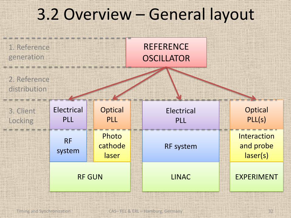
Timing and Synchronization 32
Electrical PLL
Optical PLL
Electrical PLL
Optical PLL(s)
Photo cathode
laser
Interaction and probe
laser(s)
RF system
RF system
REFERENCE OSCILLATOR
RF GUN LINAC EXPERIMENT
1. Reference generation
2. Reference distribution
3. Client Locking
CAS– FEL & ERL – Hamburg, Germany
3.2 Overview - Definitions
Timing and Synchronization 33
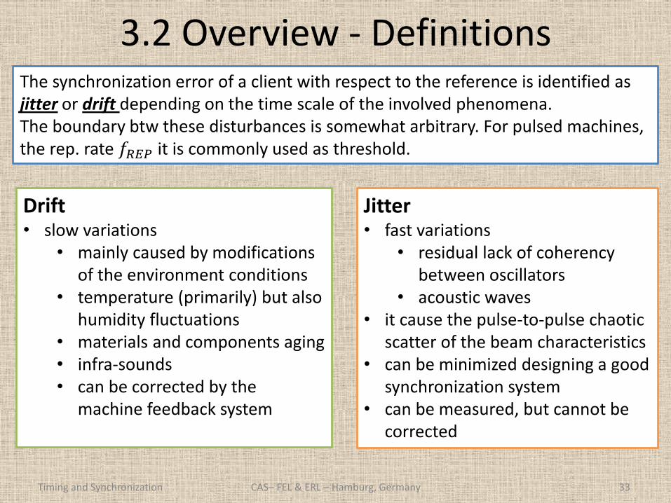
Jitter • fast variations
• residual lack of coherency between oscillators
• acoustic waves • it cause the pulse-to-pulse chaotic
scatter of the beam characteristics • can be minimized designing a good
synchronization system • can be measured, but cannot be
corrected
Drift • slow variations
• mainly caused by modifications of the environment conditions
• temperature (primarily) but also humidity fluctuations
• materials and components aging • infra-sounds • can be corrected by the
machine feedback system
The synchronization error of a client with respect to the reference is identified as jitter or drift depending on the time scale of the involved phenomena. The boundary btw these disturbances is somewhat arbitrary. For pulsed machines, the rep. rate 𝑓𝑅𝐸𝑃 it is commonly used as threshold.
CAS– FEL & ERL – Hamburg, Germany
3.2 Overview – System architecture types
Timing and Synchronization 34
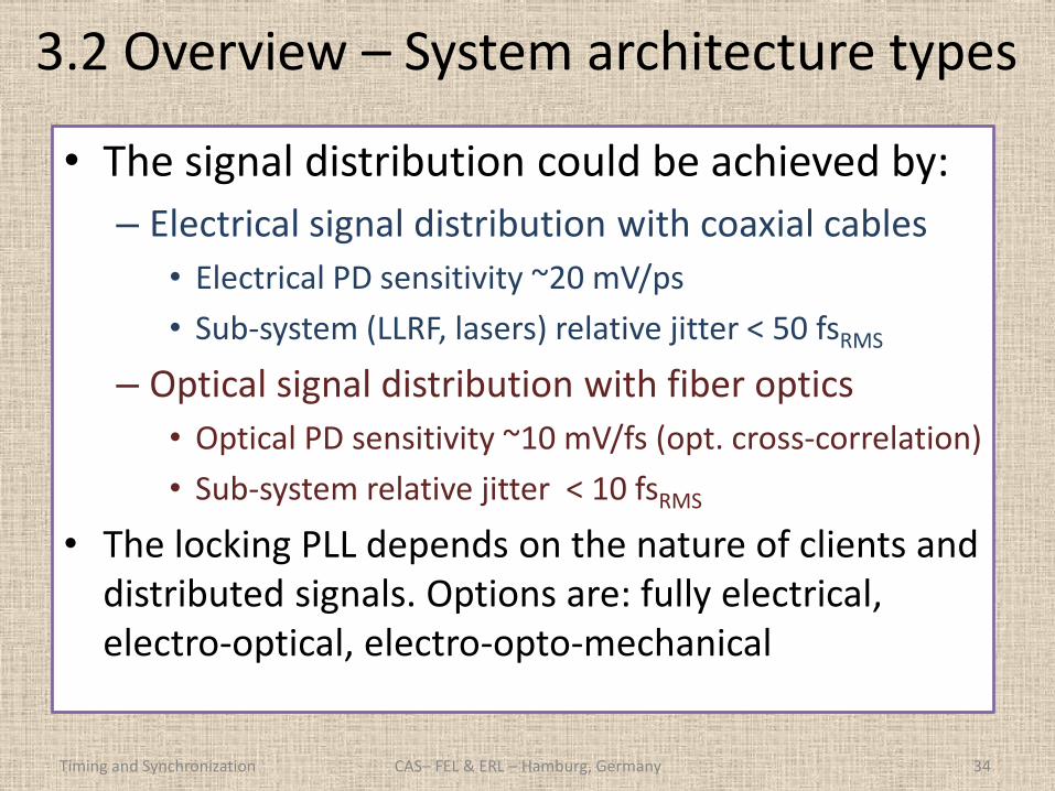
• The signal distribution could be achieved by:
– Electrical signal distribution with coaxial cables
• Electrical PD sensitivity ~20 mV/ps
• Sub-system (LLRF, lasers) relative jitter < 50 fsRMS
– Optical signal distribution with fiber optics
• Optical PD sensitivity ~10 mV/fs (opt. cross-correlation)
• Sub-system relative jitter < 10 fsRMS
• The locking PLL depends on the nature of clients and distributed signals. Options are: fully electrical, electro-optical, electro-opto-mechanical
CAS– FEL & ERL – Hamburg, Germany
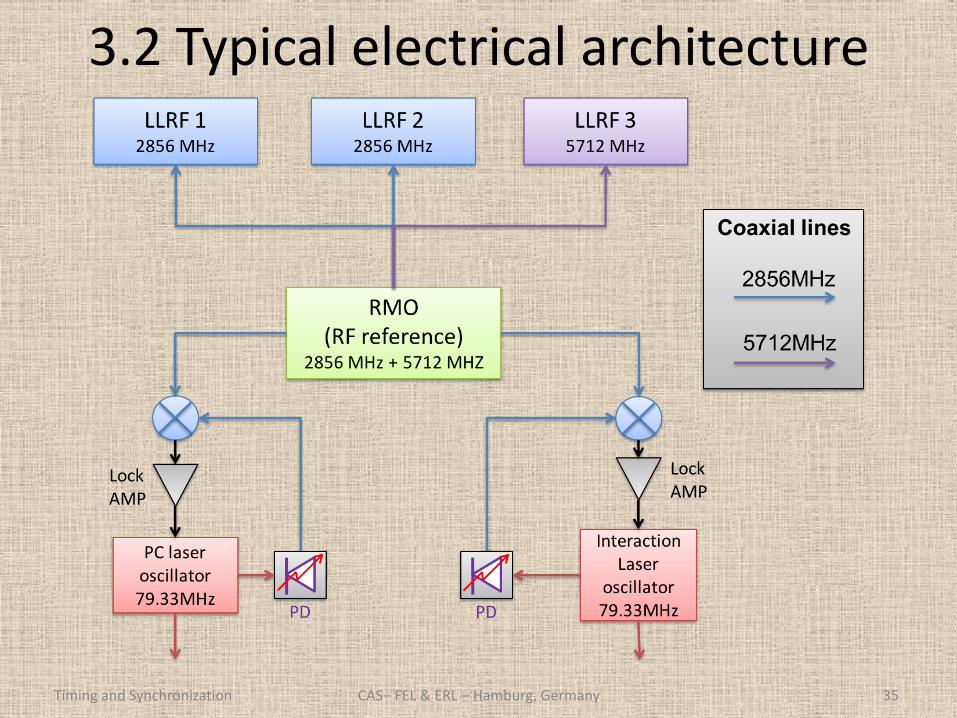
3.2 Typical electrical architecture
Timing and Synchronization 35 CAS– FEL & ERL – Hamburg, Germany
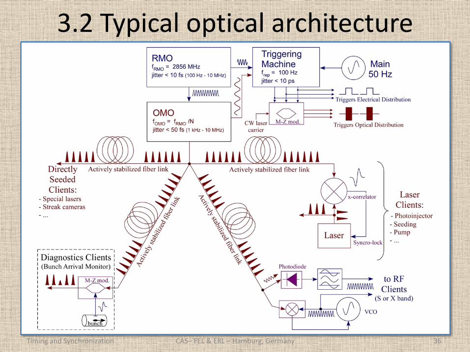
3.2 Typical optical architecture
Timing and Synchronization 36 CAS– FEL & ERL – Hamburg, Germany
;1jH
njH 2
Barkhausen’s Criterion
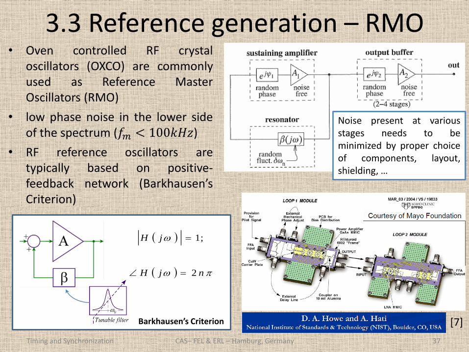
3.3 Reference generation – RMO
Timing and Synchronization 37
• Oven controlled RF crystal oscillators (OXCO) are commonly used as Reference Master Oscillators (RMO)
• low phase noise in the lower side of the spectrum (𝑓𝑚 < 100𝑘𝐻𝑧)
• RF reference oscillators are typically based on positive-feedback network (Barkhausen’s Criterion)
Noise present at various stages needs to be minimized by proper choice of components, layout, shielding, …
[7]
CAS– FEL & ERL – Hamburg, Germany
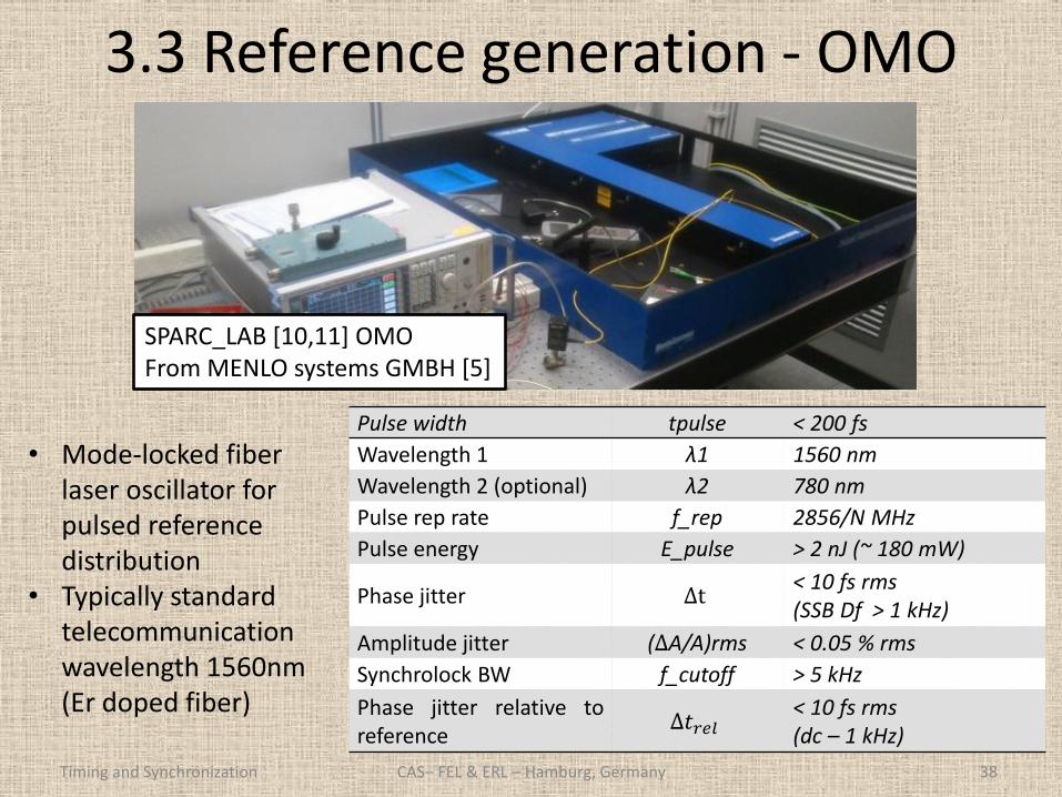
3.3 Reference generation - OMO
Timing and Synchronization 38
Pulse width tpulse < 200 fs
Wavelength 1 λ1 1560 nm
Wavelength 2 (optional) λ2 780 nm
Pulse rep rate f_rep 2856/N MHz
Pulse energy E_pulse > 2 nJ (~ 180 mW)
Phase jitter Δt < 10 fs rms (SSB Df > 1 kHz)
Amplitude jitter (ΔA/A)rms < 0.05 % rms
Synchrolock BW f_cutoff > 5 kHz
Phase jitter relative to reference
Δ𝑡𝑟𝑒𝑙 < 10 fs rms (dc – 1 kHz)
SPARC_LAB [10,11] OMO From MENLO systems GMBH [5]
• Mode-locked fiber laser oscillator for pulsed reference distribution
• Typically standard telecommunication wavelength 1560nm (Er doped fiber)
CAS– FEL & ERL – Hamburg, Germany
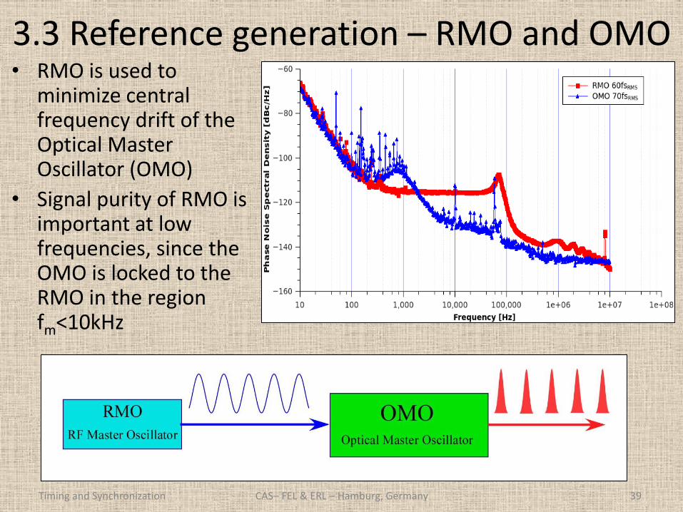
3.3 Reference generation – RMO and OMO
Timing and Synchronization 39
• RMO is used to minimize central frequency drift of the Optical Master Oscillator (OMO)
• Signal purity of RMO is important at low frequencies, since the OMO is locked to the RMO in the region fm<10kHz
CAS– FEL & ERL – Hamburg, Germany
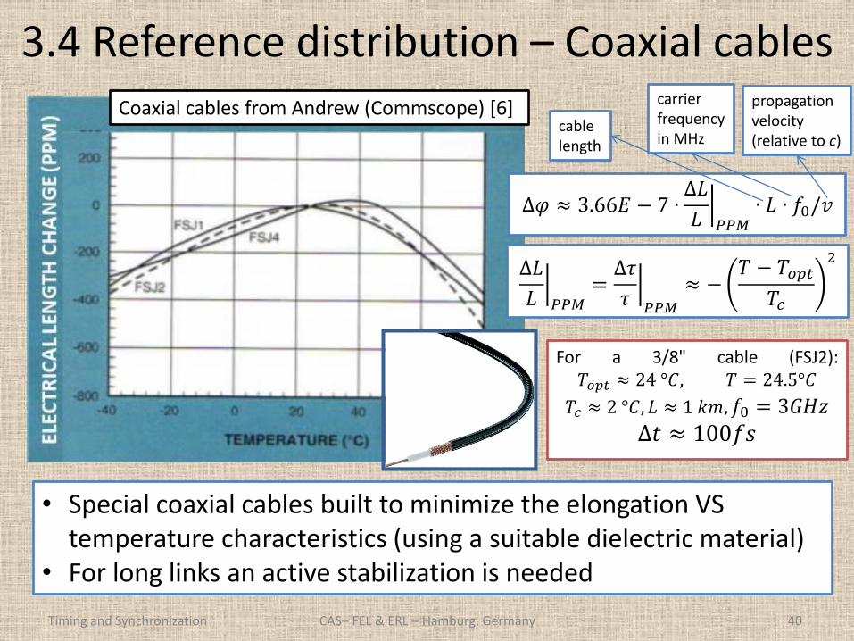
3.4 Reference distribution – Coaxial cables
Timing and Synchronization 40
Coaxial cables from Andrew (Commscope) [6]
• Special coaxial cables built to minimize the elongation VS temperature characteristics (using a suitable dielectric material)
• For long links an active stabilization is needed
∆𝐿
𝐿 𝑃𝑃𝑀
=∆𝜏
𝜏 𝑃𝑃𝑀
≈ −𝑇 − 𝑇𝑜𝑝𝑡
𝑇𝑐
2
For a 3/8" cable (FSJ2): 𝑇𝑜𝑝𝑡 ≈ 24°𝐶, 𝑇 = 24.5°𝐶
𝑇𝑐 ≈ 2°𝐶, 𝐿 ≈ 1𝑘𝑚,𝑓0 = 3𝐺𝐻𝑧 ∆𝑡 ≈ 100𝑓𝑠
∆𝜑 ≈ 3.66𝐸 − 7 ∙∆𝐿
𝐿 𝑃𝑃𝑀
∙ 𝐿 ∙ 𝑓0/𝑣
cable length
carrier frequency in MHz
propagation velocity (relative to c)
CAS– FEL & ERL – Hamburg, Germany
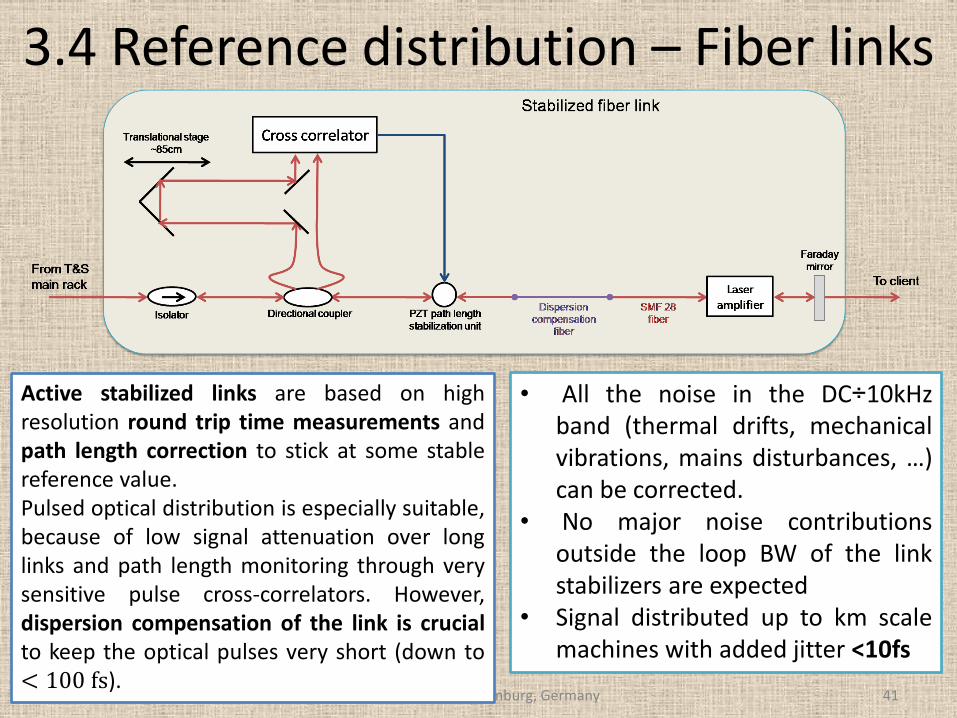
3.4 Reference distribution – Fiber links
Timing and Synchronization 41
• All the noise in the DC÷10kHz band (thermal drifts, mechanical vibrations, mains disturbances, …) can be corrected.
• No major noise contributions outside the loop BW of the link stabilizers are expected
• Signal distributed up to km scale machines with added jitter <10fs
CAS– FEL & ERL – Hamburg, Germany
Active stabilized links are based on high resolution round trip time measurements and path length correction to stick at some stable reference value. Pulsed optical distribution is especially suitable, because of low signal attenuation over long links and path length monitoring through very sensitive pulse cross-correlators. However, dispersion compensation of the link is crucial to keep the optical pulses very short (down to < 100fs).
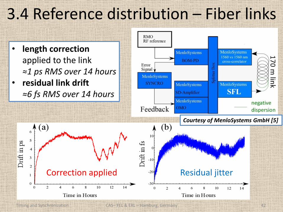
3.4 Reference distribution – Fiber links
Timing and Synchronization 42
• length correction applied to the link ≈1 ps RMS over 14 hours
• residual link drift ≈6 fs RMS over 14 hours
Correction applied Residual jitter
CAS– FEL & ERL – Hamburg, Germany
Courtesy of MenloSystems GmbH [5]
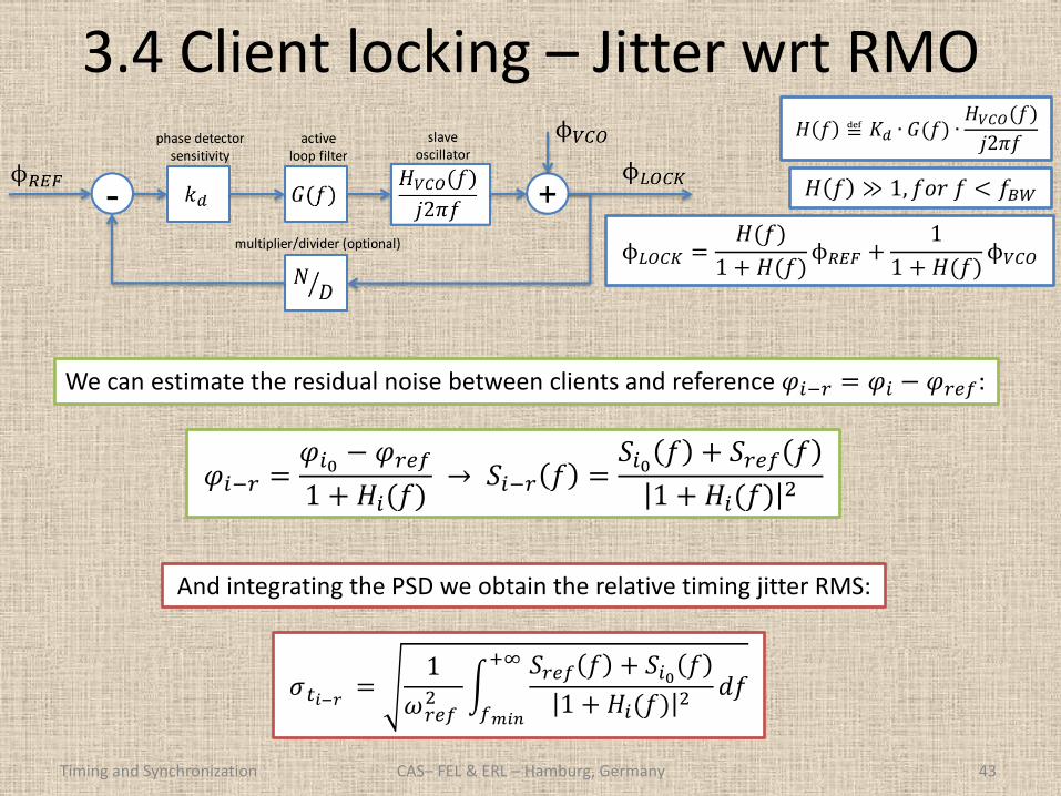
3.4 Client locking – Jitter wrt RMO
Timing and Synchronization CAS– FEL & ERL – Hamburg, Germany 43
𝐻 𝑓 ≫ 1, 𝑓𝑜𝑟𝑓 < 𝑓𝐵𝑊
𝜑𝑖−𝑟 =𝜑𝑖0 − 𝜑𝑟𝑒𝑓
1 + 𝐻𝑖(𝑓)→ 𝑆𝑖−𝑟 𝑓 =
𝑆𝑖0 𝑓 + 𝑆𝑟𝑒𝑓 𝑓
1 + 𝐻𝑖(𝑓) 2
We can estimate the residual noise between clients and reference 𝜑𝑖−𝑟 = 𝜑𝑖 − 𝜑𝑟𝑒𝑓:
𝜎 𝑡𝑖−𝑟
=1
𝜔 𝑟𝑒𝑓2
𝑆𝑟𝑒𝑓 𝑓 + 𝑆𝑖0 𝑓
1 + 𝐻𝑖(𝑓) 2
+∞
𝑓𝑚𝑖𝑛
𝑑𝑓
And integrating the PSD we obtain the relative timing jitter RMS:
ϕ𝐿𝑂𝐶𝐾 =𝐻(𝑓)
1 + 𝐻(𝑓)ϕ𝑅𝐸𝐹 +
1
1 + 𝐻(𝑓)ϕ𝑉𝐶𝑂
𝐻 𝑓 ≝ 𝐾𝑑 ∙ 𝐺(𝑓) ∙𝐻𝑉𝐶𝑂(𝑓)
𝑗2𝜋𝑓
𝜑𝑖−𝑗 = 𝜑𝑖−𝑟 − 𝜑𝑗−𝑟 =𝜑𝑖0 − 𝜑𝑟𝑒𝑓
1 + 𝐻𝑖(𝑓)−
𝜑𝑗0− 𝜑𝑟𝑒𝑓
1 + 𝐻𝑗(𝑓)
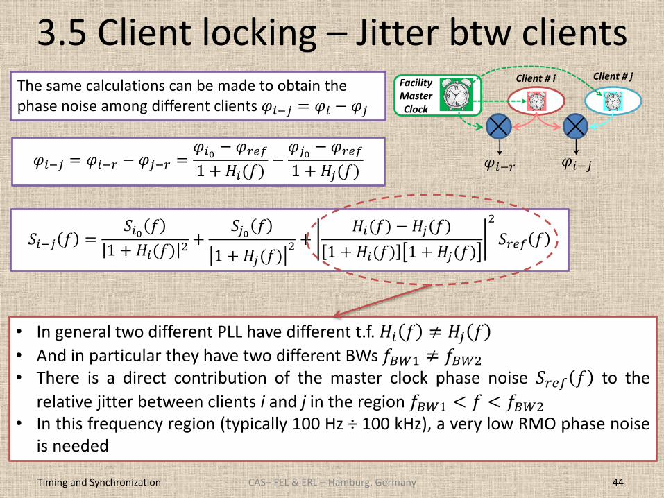
3.5 Client locking – Jitter btw clients
Timing and Synchronization 44
Facility Master Clock
Client # i Client # j
𝜑𝑖−𝑟 𝜑𝑖−𝑗
• In general two different PLL have different t.f.𝐻𝑖 𝑓 ≠ 𝐻𝑗 𝑓
• And in particular they have two different BWs 𝑓𝐵𝑊1 ≠ 𝑓𝐵𝑊2 • There is a direct contribution of the master clock phase noise 𝑆𝑟𝑒𝑓 𝑓 to the
relative jitter between clients i and j in the region 𝑓𝐵𝑊1 < 𝑓 < 𝑓𝐵𝑊2 • In this frequency region (typically 100 Hz ÷ 100 kHz), a very low RMO phase noise
is needed
The same calculations can be made to obtain the phase noise among different clients 𝜑𝑖−𝑗 = 𝜑𝑖 − 𝜑𝑗
𝑆𝑖−𝑗 𝑓 =𝑆𝑖0 𝑓
1 + 𝐻𝑖(𝑓) 2 +𝑆𝑗0
𝑓
1 + 𝐻𝑗(𝑓)2 +
𝐻𝑖(𝑓) − 𝐻𝑗(𝑓)
1 + 𝐻𝑖(𝑓) 1 + 𝐻𝑗(𝑓)
2
𝑆𝑟𝑒𝑓 𝑓
CAS– FEL & ERL – Hamburg, Germany
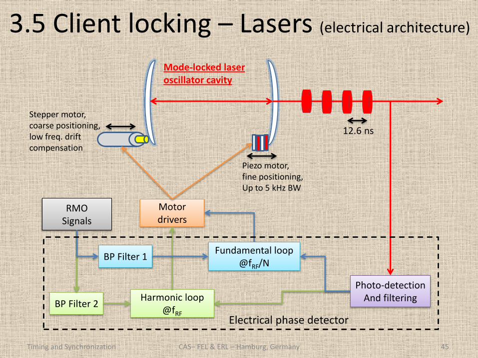
3.5 Client locking – Lasers (electrical architecture)
Timing and Synchronization 45
Stepper motor, coarse positioning, low freq. drift compensation
Piezo motor, fine positioning, Up to 5 kHz BW
12.6 ns
Motor drivers
Harmonic loop @fRF
RMO Signals
Fundamental loop @fRF/N
BP Filter 2
Mode-locked laser oscillator cavity
BP Filter 1
Photo-detection And filtering
Electrical phase detector
CAS– FEL & ERL – Hamburg, Germany
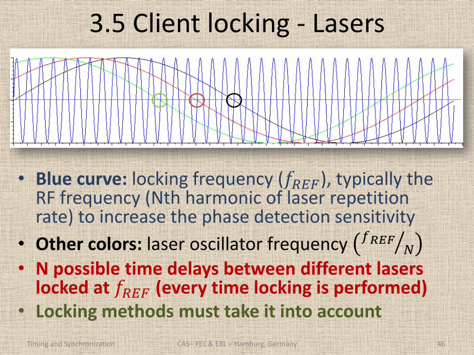
3.5 Client locking - Lasers
Timing and Synchronization 46
• Blue curve: locking frequency (𝑓𝑅𝐸𝐹), typically the RF frequency (Nth harmonic of laser repetition rate) to increase the phase detection sensitivity
• Other colors: laser oscillator frequency 𝑓𝑅𝐸𝐹𝑁
• N possible time delays between different lasers locked at 𝑓𝑅𝐸𝐹 (every time locking is performed)
• Locking methods must take it into account
CAS– FEL & ERL – Hamburg, Germany
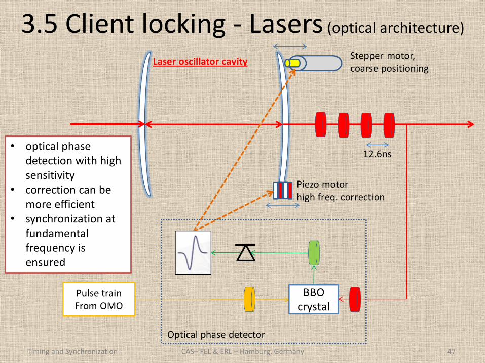
3.5 Client locking - Lasers (optical architecture)
Timing and Synchronization 47 CAS– FEL & ERL – Hamburg, Germany
• optical phase detection with high sensitivity
• correction can be more efficient
• synchronization at fundamental frequency is ensured
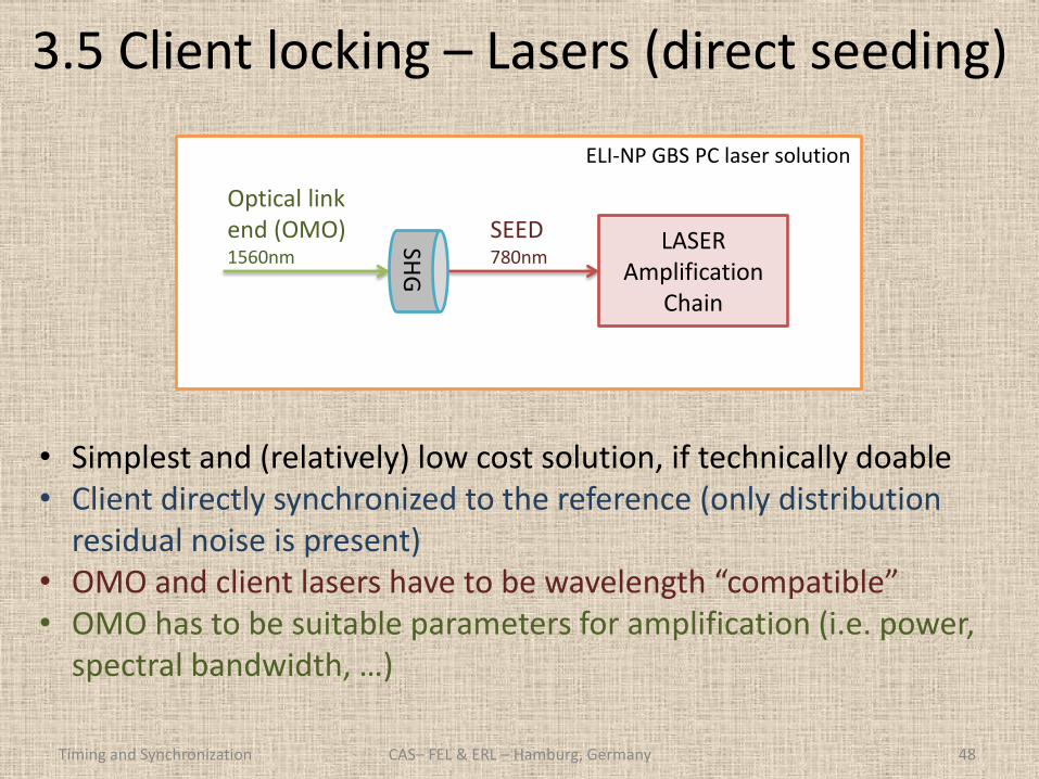
3.5 Client locking – Lasers (direct seeding)
Timing and Synchronization 48
Optical link end (OMO) 1560nm
SEED 780nm
SHG
LASER Amplification
Chain
ELI-NP GBS PC laser solution
• Simplest and (relatively) low cost solution, if technically doable • Client directly synchronized to the reference (only distribution
residual noise is present) • OMO and client lasers have to be wavelength “compatible” • OMO has to be suitable parameters for amplification (i.e. power,
spectral bandwidth, …)
CAS– FEL & ERL – Hamburg, Germany
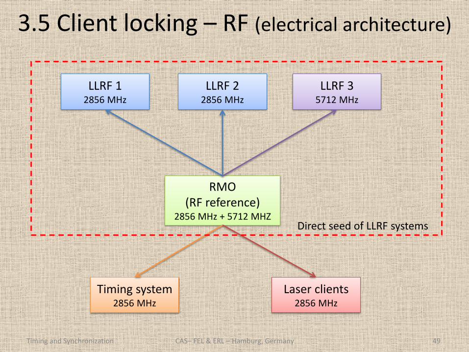
3.5 Client locking – RF (electrical architecture)
Timing and Synchronization 49
LLRF 1 2856 MHz
LLRF 2 2856 MHz
LLRF 3 5712 MHz
RMO (RF reference)
2856 MHz + 5712 MHZ
Timing system 2856 MHz
Laser clients 2856 MHz
Direct seed of LLRF systems
CAS– FEL & ERL – Hamburg, Germany
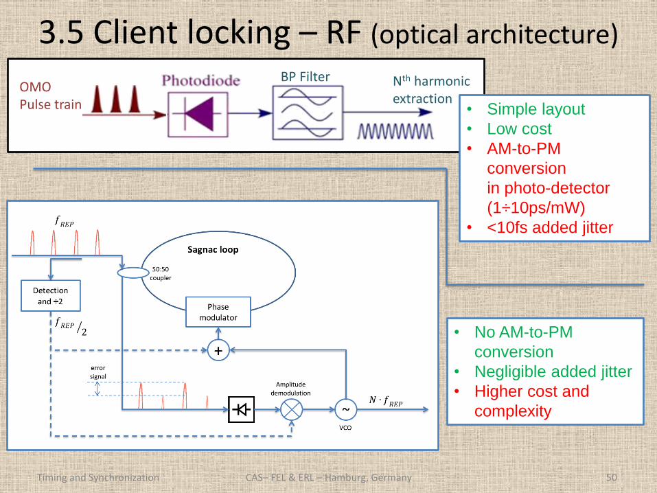
3.5 Client locking – RF (optical architecture)
Timing and Synchronization 50
OMO Pulse train
BP Filter Nth harmonic extraction
• Simple layout
• Low cost
• AM-to-PM
conversion
in photo-detector
(1÷10ps/mW)
• <10fs added jitter
• No AM-to-PM
conversion
• Negligible added jitter
• Higher cost and
complexity
CAS– FEL & ERL – Hamburg, Germany
3.6 Beam timing jitter - Sources
Timing and Synchronization 51
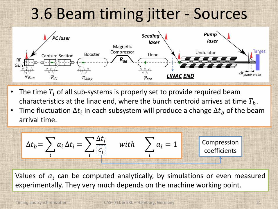
• The time 𝑇𝑖 of all sub-systems is properly set to provide required beam characteristics at the linac end, where the bunch centroid arrives at time 𝑇𝑏.
• Time fluctuation ∆𝑡𝑖 in each subsystem will produce a change ∆𝑡𝑏 of the beam arrival time.
PC laser Seeding laser
Pump laser
LINAC END
R56
∆𝑡𝑏= 𝑎𝑖
𝑖
∆𝑡𝑖 = ∆𝑡𝑖
𝑐𝑖𝑖
𝑤𝑖𝑡 𝑎𝑖
𝑖
= 1 Compression coefficients
Values of 𝑎𝑖 can be computed analytically, by simulations or even measured experimentally. They very much depends on the machine working point.
CAS– FEL & ERL – Hamburg, Germany
3.6 Beam timing jitter - Sources
Timing and Synchronization 52
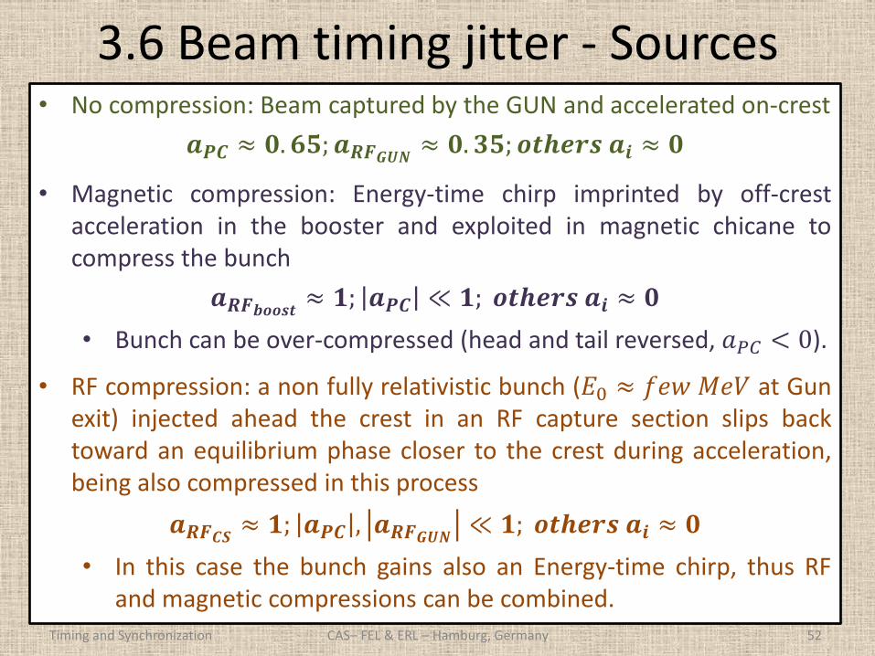
• No compression: Beam captured by the GUN and accelerated on-crest
𝒂𝑷𝑪 ≈ 𝟎. 𝟔𝟓; 𝒂𝑹𝑭𝑮𝑼𝑵≈ 𝟎. 𝟑𝟓; 𝒐𝒕𝒉𝒆𝒓𝒔𝒂𝒊 ≈ 𝟎
• Magnetic compression: Energy-time chirp imprinted by off-crest acceleration in the booster and exploited in magnetic chicane to compress the bunch
𝒂𝑹𝑭𝒃𝒐𝒐𝒔𝒕≈ 𝟏; 𝒂𝑷𝑪 ≪ 𝟏; 𝒐𝒕𝒉𝒆𝒓𝒔𝒂𝒊 ≈ 𝟎
• Bunch can be over-compressed (head and tail reversed, 𝑎𝑃𝐶 < 0).
• RF compression: a non fully relativistic bunch (𝐸0 ≈ 𝑓𝑒𝑤𝑀𝑒𝑉 at Gun exit) injected ahead the crest in an RF capture section slips back toward an equilibrium phase closer to the crest during acceleration, being also compressed in this process
𝒂𝑹𝑭𝑪𝑺≈ 𝟏; 𝒂𝑷𝑪 , 𝒂𝑹𝑭𝑮𝑼𝑵
≪ 𝟏; 𝒐𝒕𝒉𝒆𝒓𝒔𝒂𝒊 ≈ 𝟎
• In this case the bunch gains also an Energy-time chirp, thus RF and magnetic compressions can be combined.
CAS– FEL & ERL – Hamburg, Germany
3.6 Beam timing jitter – Relative jitter
Timing and Synchronization 53
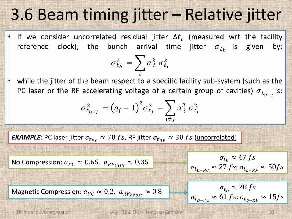
𝜎𝑡𝑏≈ 28𝑓𝑠
𝜎𝑡𝑏−𝑃𝐶≈ 61𝑓𝑠; 𝜎𝑡𝑏−𝑅𝐹
≈ 15𝑓𝑠
𝜎𝑡𝑏≈ 47𝑓𝑠
𝜎𝑡𝑏−𝑃𝐶≈ 27𝑓𝑠; 𝜎𝑡𝑏−𝑅𝐹
≈ 50𝑓𝑠
• If we consider uncorrelated residual jitter ∆𝑡𝑖 (measured wrt the facility reference clock), the bunch arrival time jitter 𝜎 𝑡𝑏
is given by:
𝜎 𝑡𝑏2 = 𝑎 𝑖
2
𝑖
𝜎 𝑡𝑖2
• while the jitter of the beam respect to a specific facility sub-system (such as the PC laser or the RF accelerating voltage of a certain group of cavities) 𝜎 𝑡𝑏−𝑗
is:
𝜎 𝑡𝑏−𝑗2 = 𝑎𝑗 − 1
2𝜎 𝑡𝑗
2 + 𝑎 𝑖2
𝑖≠𝑗
𝜎 𝑡𝑖2
EXAMPLE: PC laser jitter 𝜎𝑡𝑃𝐶≈ 70𝑓𝑠, RF jitter 𝜎𝑡𝑅𝐹
≈ 30𝑓𝑠 (uncorrelated)
CAS– FEL & ERL – Hamburg, Germany
No Compression: 𝑎𝑃𝐶 ≈ 0.65, 𝑎𝑅𝐹𝐺𝑈𝑁≈ 0.35
Magnetic Compression: 𝑎𝑃𝐶 ≈ 0.2, 𝑎𝑅𝐹𝑏𝑜𝑜𝑠𝑡≈ 0.8
3.7 Diagnostics – LLRF phase noise detection
Timing and Synchronization 54
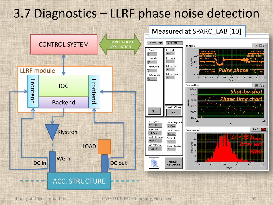
Δt ≈ 55 fsRMS
Jitter wrt RMO
Pulse phase
Shot-by-shot Phase time chart
Measured at SPARC_LAB [10]
CAS– FEL & ERL – Hamburg, Germany
ACC. STRUCTURE
LOAD
Klystron
IOC
Backend
Fron
tend
Fron
tend
DC in DC out
CONTROL SYSTEM CONROL ROOM APPLICATION
WG in
LLRF module
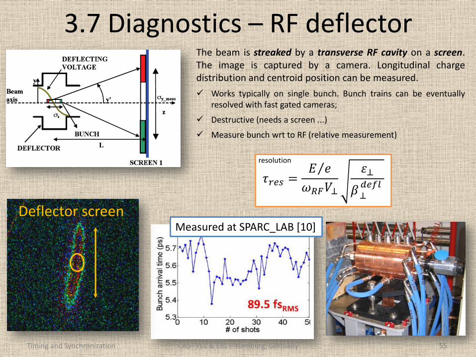
3.7 Diagnostics – RF deflector
Timing and Synchronization 55
Deflector screen
The beam is streaked by a transverse RF cavity on a screen. The image is captured by a camera. Longitudinal charge distribution and centroid position can be measured.
Works typically on single bunch. Bunch trains can be eventually resolved with fast gated cameras;
Destructive (needs a screen ...)
Measure bunch wrt to RF (relative measurement)
𝜏𝑟𝑒𝑠 =𝐸 𝑒
𝜔𝑅𝐹𝑉⊥
𝜀⊥
𝛽 ⊥𝑑𝑒𝑓𝑙
Measured at SPARC_LAB [10]
CAS– FEL & ERL – Hamburg, Germany
resolution
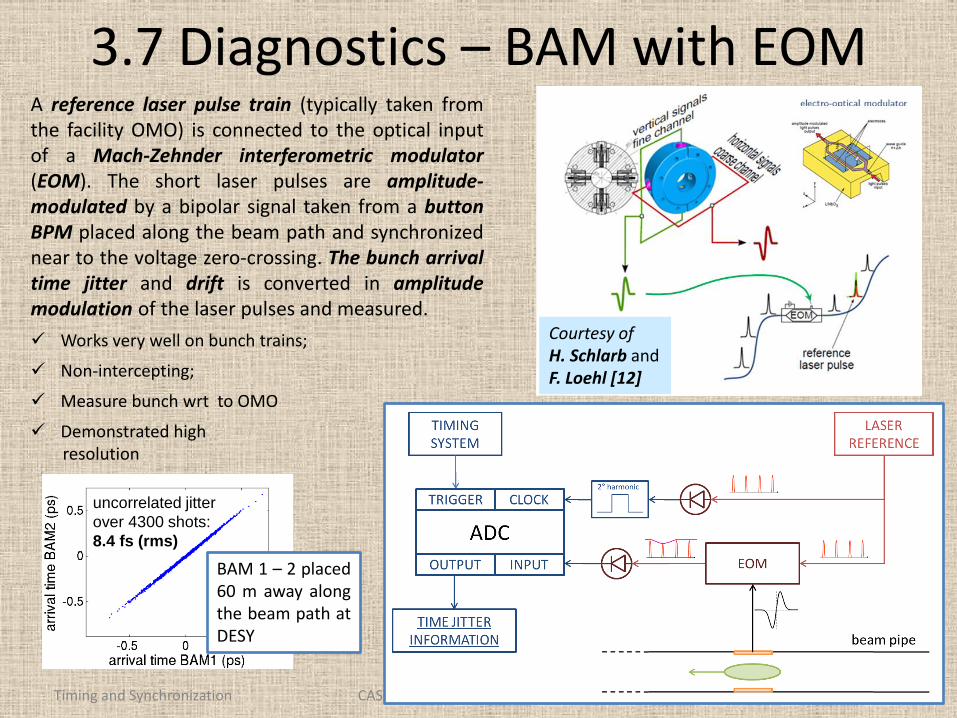
3.7 Diagnostics – BAM with EOM
Timing and Synchronization 56
uncorrelated jitter
over 4300 shots:
8.4 fs (rms)
A reference laser pulse train (typically taken from the facility OMO) is connected to the optical input of a Mach-Zehnder interferometric modulator (EOM). The short laser pulses are amplitude-modulated by a bipolar signal taken from a button BPM placed along the beam path and synchronized near to the voltage zero-crossing. The bunch arrival time jitter and drift is converted in amplitude modulation of the laser pulses and measured.
Works very well on bunch trains;
Non-intercepting;
Measure bunch wrt to OMO
Demonstrated high resolution
BAM 1 – 2 placed 60 m away along the beam path at DESY
Courtesy of H. Schlarb and F. Loehl [12]
CAS– FEL & ERL – Hamburg, Germany
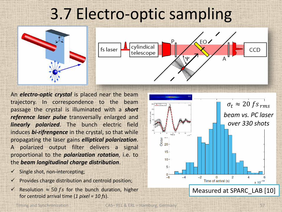
3.7 Electro-optic sampling
Timing and Synchronization 57
𝜎𝑡 ≈ 20𝑓𝑠𝑟𝑚𝑠
beam vs. PC laser over 330 shots
An electro-optic crystal is placed near the beam trajectory. In correspondence to the beam passage the crystal is illuminated with a short reference laser pulse transversally enlarged and linearly polarized. The bunch electric field induces bi-rifrengence in the crystal, so that while propagating the laser gains elliptical polarization. A polarized output filter delivers a signal proportional to the polarization rotation, i.e. to the beam longitudinal charge distribution.
Single shot, non-intercepting;
Provides charge distribution and centroid position;
Resolution ≈ 50𝑓𝑠 for the bunch duration, higher for centroid arrival time (1 pixel ≈ 10 fs).
Measured at SPARC_LAB [10]
CAS– FEL & ERL – Hamburg, Germany
Timing and Synchronization 58
4. Timing in linear injectors
CAS– FEL & ERL – Hamburg, Germany
1. Overview
2. Timing signals generation
3. Timing signals distribution
4. Timing example - Typical event sequence
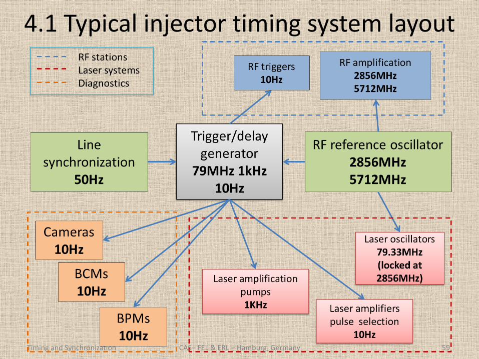
4.1 Typical injector timing system layout
Timing and Synchronization 59 CAS– FEL & ERL – Hamburg, Germany
4.2 Timing signals generation
Timing and Synchronization 60
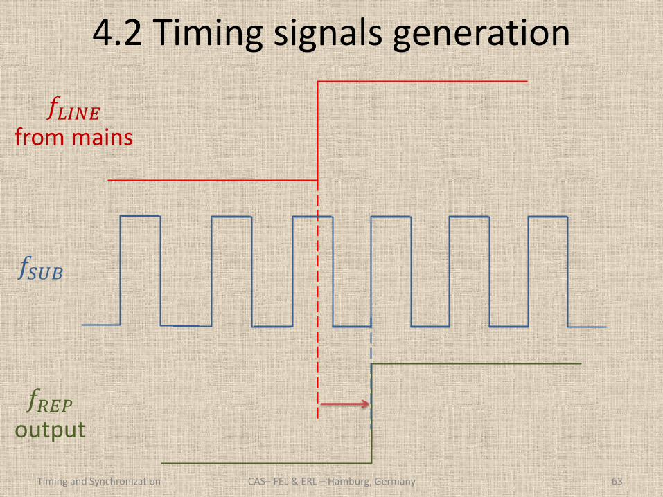
• The machine trigger generator is mainly a frequency divider
• Typically it divides one output of the RMO (𝑓𝑅𝑀𝑂) at different stages to generate all the desired sub-harmonics, down to the machine rep. rate (𝑓𝑅𝐸𝑃)
• The resulting jitter is 10ps ÷10ns depending of the divider stage
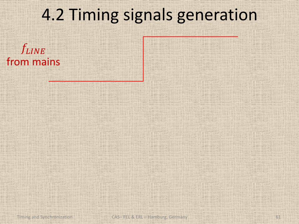
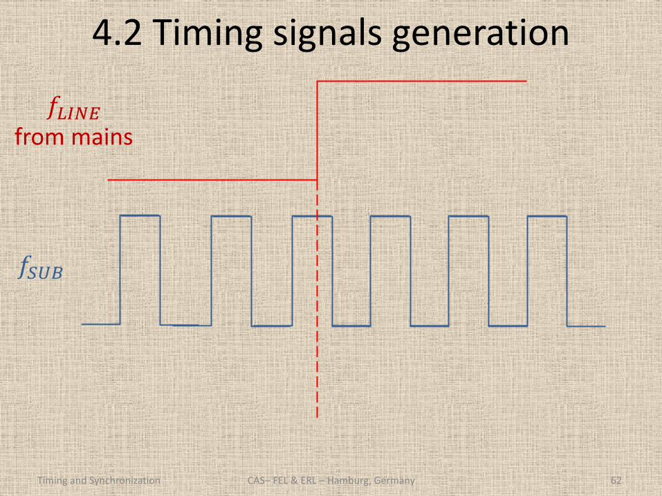
• It also take the 50Hz mains input and generate from it a signal at 𝑓𝑅𝐸𝑃 (either dividing or multiplying). We call it 𝑓𝐿𝐼𝑁𝐸
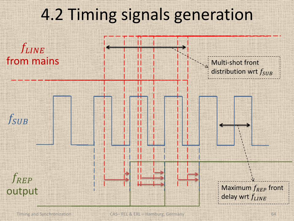
• The final machine clock is generated selecting the first logic front of one 𝑓𝑅𝑀𝑂 sub-harmonic (𝑓𝑆𝑈𝐵) following a 𝑓𝐿𝐼𝑁𝐸 front (reducing magnet power supply current ripple)
• 𝑓𝑆𝑈𝐵 must be coherent with all the system clocks (lasers rep. rate, ADC and DAC sample clocks, …) to avoid trigger edge slippage/jumps
CAS– FEL & ERL – Hamburg, Germany
4.2 Timing signals generation
Timing and Synchronization 61
𝑓𝐿𝐼𝑁𝐸 from mains
CAS– FEL & ERL – Hamburg, Germany
4.2 Timing signals generation
Timing and Synchronization 62
𝑓𝐿𝐼𝑁𝐸 from mains
𝑓𝑆𝑈𝐵
CAS– FEL & ERL – Hamburg, Germany
4.2 Timing signals generation
Timing and Synchronization 63
𝑓𝐿𝐼𝑁𝐸 from mains
𝑓𝑆𝑈𝐵
𝑓𝑅𝐸𝑃 output
CAS– FEL & ERL – Hamburg, Germany
4.2 Timing signals generation
Timing and Synchronization 64
𝑓𝐿𝐼𝑁𝐸 from mains
𝑓𝑆𝑈𝐵
𝑓𝑅𝐸𝑃 output
CAS– FEL & ERL – Hamburg, Germany
Multi-shot front distribution wrt 𝑓𝑆𝑈𝐵
Maximum 𝑓𝑅𝐸𝑃front delay wrt 𝑓𝐿𝐼𝑁𝐸
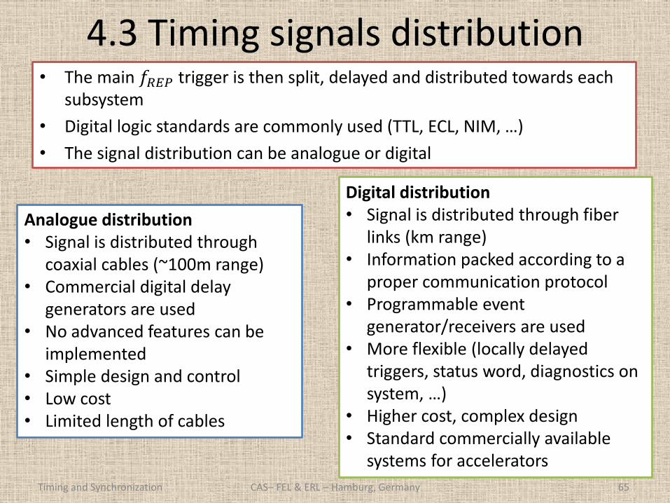
4.3 Timing signals distribution • The main 𝑓𝑅𝐸𝑃 trigger is then split, delayed and distributed towards each
subsystem
• Digital logic standards are commonly used (TTL, ECL, NIM, …)
• The signal distribution can be analogue or digital
Timing and Synchronization 65
Digital distribution • Signal is distributed through fiber
links (km range) • Information packed according to a
proper communication protocol • Programmable event
generator/receivers are used • More flexible (locally delayed
triggers, status word, diagnostics on system, …)
• Higher cost, complex design • Standard commercially available
systems for accelerators
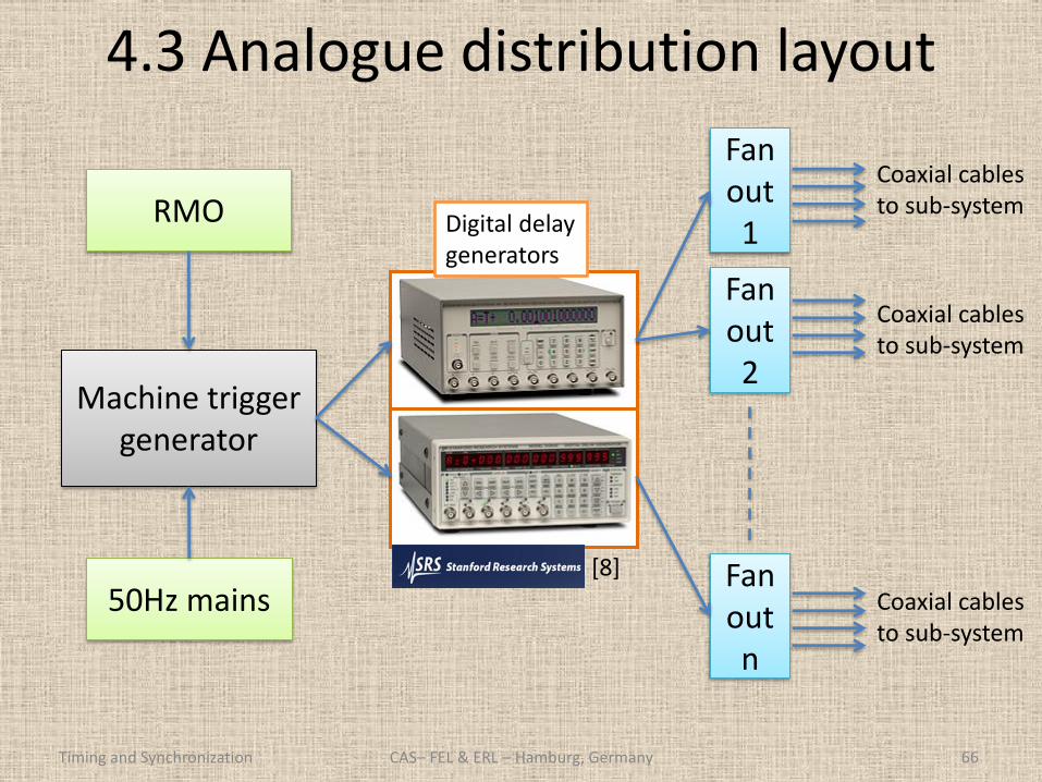
Analogue distribution • Signal is distributed through
coaxial cables (~100m range) • Commercial digital delay
generators are used • No advanced features can be
implemented • Simple design and control • Low cost • Limited length of cables
CAS– FEL & ERL – Hamburg, Germany
4.3 Analogue distribution layout
Timing and Synchronization 66
[8]
RMO
Machine trigger generator
Fanout 1
Fanout n
Fanout 2
Digital delay generators
Coaxial cables to sub-system
Coaxial cables to sub-system
Coaxial cables to sub-system
CAS– FEL & ERL – Hamburg, Germany
50Hz mains
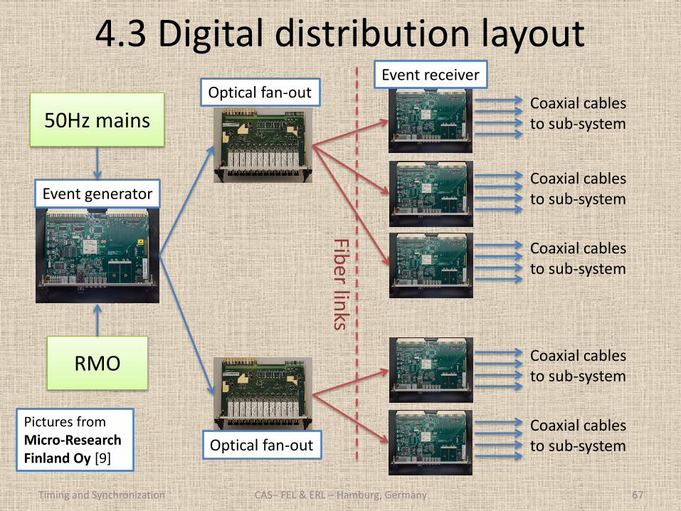
4.3 Digital distribution layout
Timing and Synchronization 67
Event generator
Optical fan-out
RMO Fib
er links
Event receiver
Coaxial cables to sub-system
Coaxial cables to sub-system
Coaxial cables to sub-system
Coaxial cables to sub-system
Coaxial cables to sub-system
CAS– FEL & ERL – Hamburg, Germany
50Hz mains
Optical fan-out
Pictures from Micro-Research Finland Oy [9]
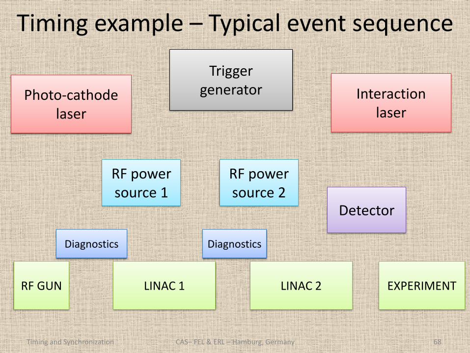
Timing example – Typical event sequence
Timing and Synchronization CAS– FEL & ERL – Hamburg, Germany 68
Photo-cathode laser
Trigger generator
RF GUN LINAC 1 EXPERIMENT LINAC 2
Detector
RF power source 1
RF power source 2
Interaction laser
Diagnostics Diagnostics
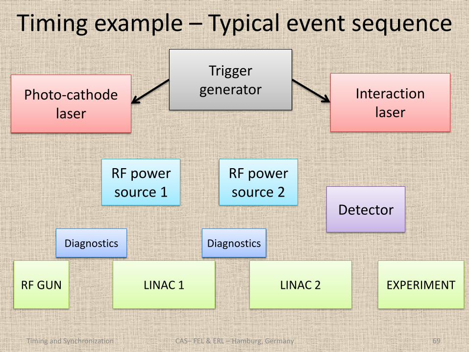
Timing example – Typical event sequence
Timing and Synchronization CAS– FEL & ERL – Hamburg, Germany 69
Photo-cathode laser
Trigger generator
RF GUN LINAC 1 EXPERIMENT LINAC 2
Detector
RF power source 1
RF power source 2
Interaction laser
Diagnostics Diagnostics
Diagnostics Diagnostics
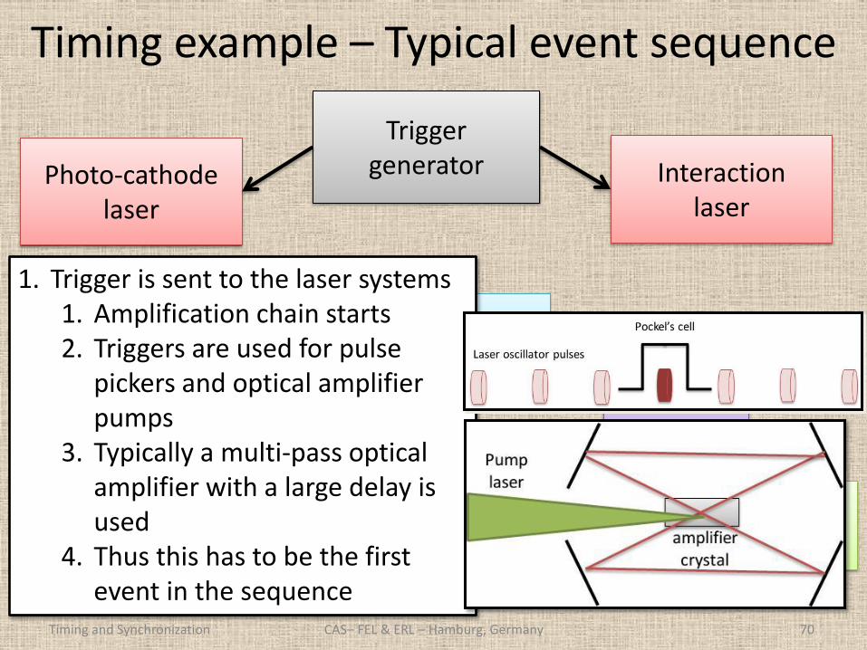
Timing example – Typical event sequence
Timing and Synchronization CAS– FEL & ERL – Hamburg, Germany 70
Photo-cathode laser
Trigger generator
RF GUN LINAC 1 EXPERIMENT LINAC 2
Detector
RF power source 1
RF power source 2
Interaction laser
1. Trigger is sent to the laser systems 1. Amplification chain starts 2. Triggers are used for pulse
pickers and optical amplifier pumps
3. Typically a multi-pass optical amplifier with a large delay is used
4. Thus this has to be the first event in the sequence
Diagnostics Diagnostics
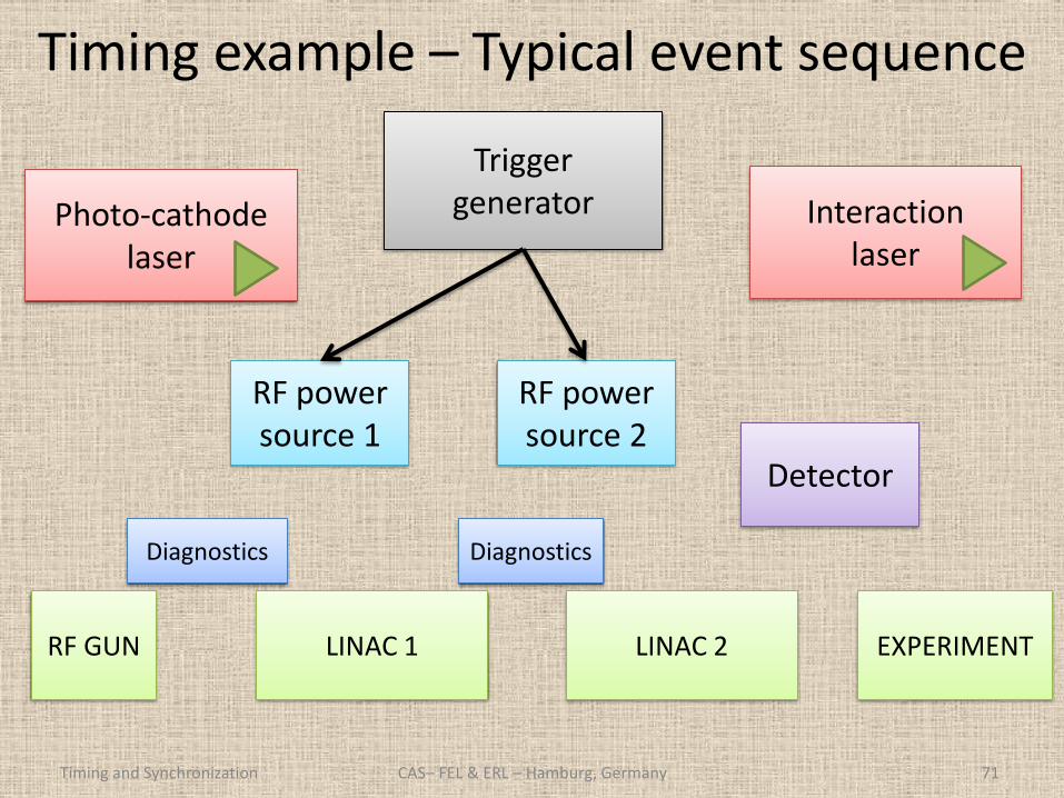
Timing example – Typical event sequence
Timing and Synchronization CAS– FEL & ERL – Hamburg, Germany 71
Photo-cathode laser
Trigger generator
RF GUN LINAC 1 EXPERIMENT LINAC 2
Detector
RF power source 1
RF power source 2
Interaction laser
Diagnostics Diagnostics
Timing example – Typical event sequence
Timing and Synchronization CAS– FEL & ERL – Hamburg, Germany 72
Photo-cathode laser
Trigger generator
RF GUN LINAC 1 EXPERIMENT LINAC 2
Detector
RF power source 1
RF power source 2
Interaction laser
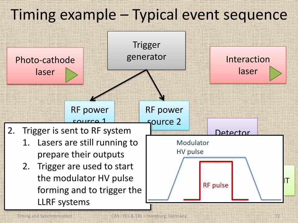
2. Trigger is sent to RF system 1. Lasers are still running to
prepare their outputs 2. Trigger are used to start
the modulator HV pulse forming and to trigger the LLRF systems
Diagnostics Diagnostics
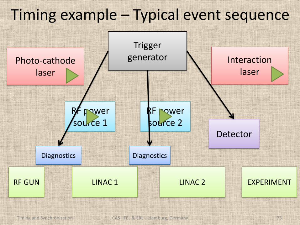
Timing example – Typical event sequence
Timing and Synchronization CAS– FEL & ERL – Hamburg, Germany 73
Photo-cathode laser
Trigger generator
RF GUN LINAC 1 EXPERIMENT LINAC 2
Detector
RF power source 1
RF power source 2
Interaction laser
Diagnostics Diagnostics
Timing example – Typical event sequence
Timing and Synchronization CAS– FEL & ERL – Hamburg, Germany 74
Photo-cathode laser
Trigger generator
RF GUN LINAC 1 EXPERIMENT LINAC 2
Detector
RF power source 1
RF power source 2
Interaction laser
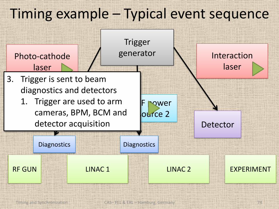
3. Trigger is sent to beam diagnostics and detectors 1. Trigger are used to arm
cameras, BPM, BCM and detector acquisition
Diagnostics Diagnostics
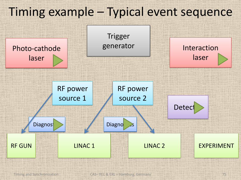
Timing example – Typical event sequence
Timing and Synchronization CAS– FEL & ERL – Hamburg, Germany 75
Photo-cathode laser
Trigger generator
RF GUN LINAC 1 EXPERIMENT LINAC 2
Detector
RF power source 1
RF power source 2
Interaction laser
Diagnostics Diagnostics
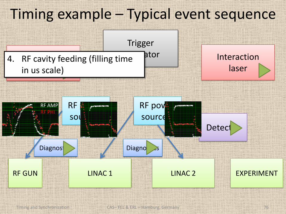
Timing example – Typical event sequence
Timing and Synchronization CAS– FEL & ERL – Hamburg, Germany 76
Photo-cathode laser
Trigger generator
RF GUN LINAC 1 EXPERIMENT LINAC 2
Detector
RF power source 1
RF power source 2
Interaction laser
4. RF cavity feeding (filling time in us scale)
RF AMP RF PHI
Diagnostics Diagnostics
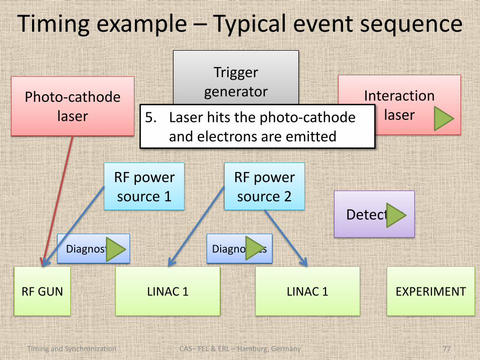
Timing example – Typical event sequence
Timing and Synchronization CAS– FEL & ERL – Hamburg, Germany 77
Photo-cathode laser
Trigger generator
RF GUN LINAC 1 EXPERIMENT LINAC 1
Detector
RF power source 1
RF power source 2
Interaction laser 5. Laser hits the photo-cathode
and electrons are emitted
Diagnostics Diagnostics
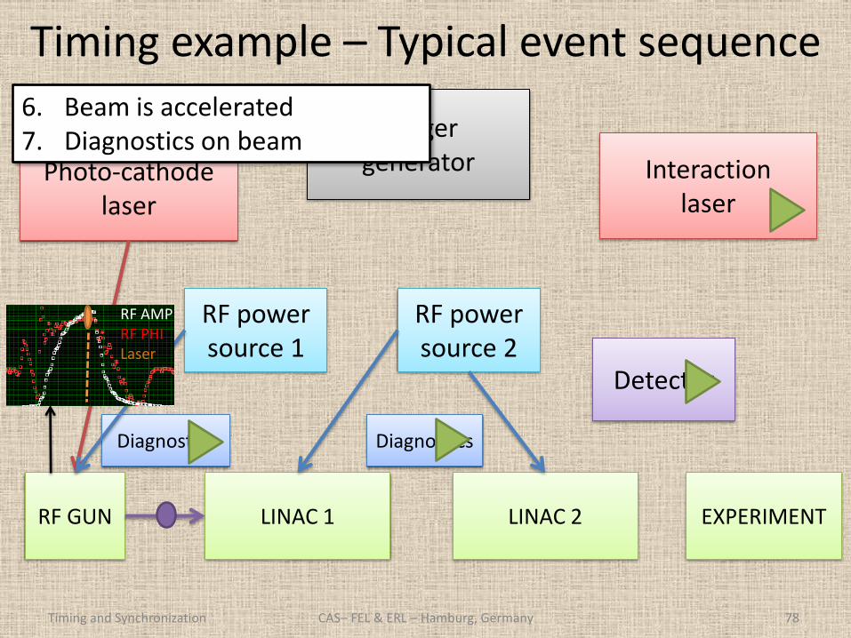
Timing example – Typical event sequence
Timing and Synchronization CAS– FEL & ERL – Hamburg, Germany 78
Photo-cathode laser
Trigger generator
RF GUN LINAC 1 EXPERIMENT LINAC 2
Detector
RF power source 1
RF power source 2
Interaction laser
6. Beam is accelerated 7. Diagnostics on beam
RF AMP RF PHI Laser
Diagnostics Diagnostics
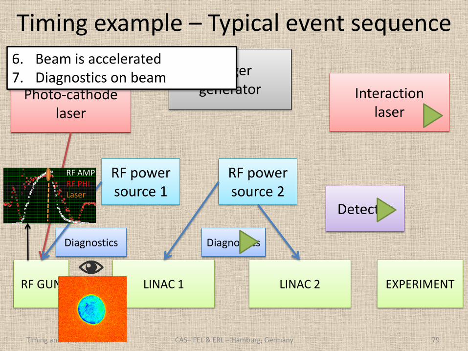
Timing example – Typical event sequence
Timing and Synchronization CAS– FEL & ERL – Hamburg, Germany 79
Photo-cathode laser
Trigger generator
RF GUN LINAC 1 EXPERIMENT LINAC 2
Detector
RF power source 1
RF power source 2
Interaction laser
RF AMP RF PHI Laser
6. Beam is accelerated 7. Diagnostics on beam
Diagnostics Diagnostics
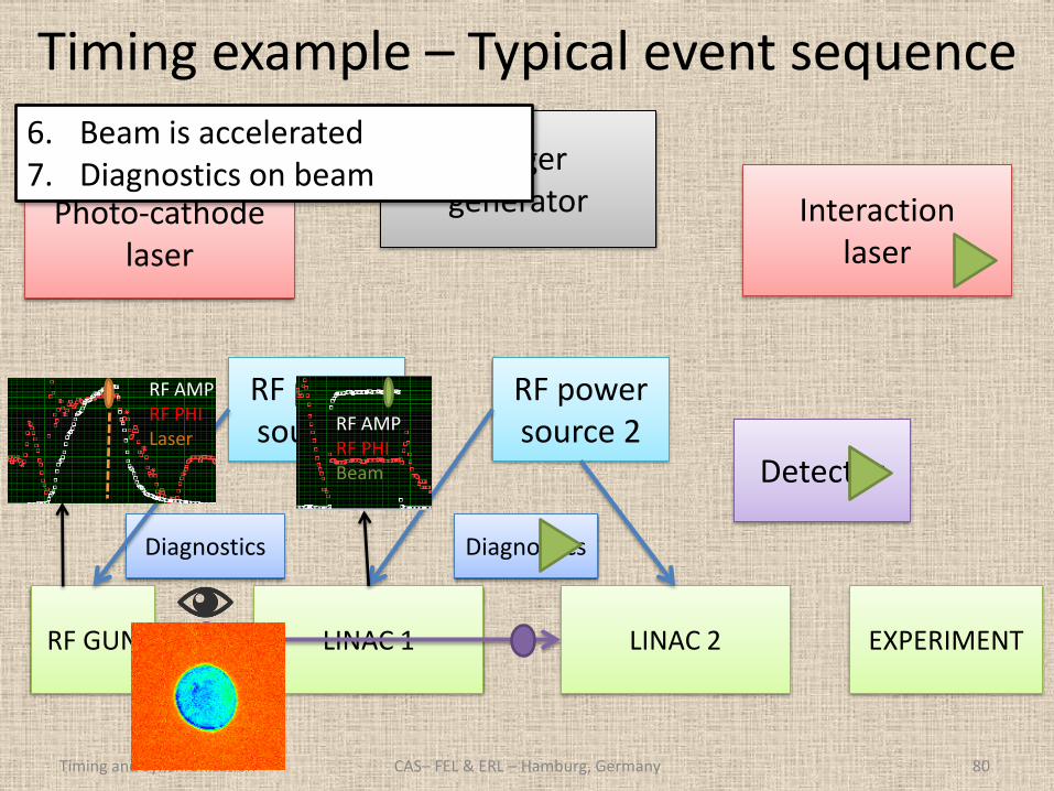
Timing example – Typical event sequence
Timing and Synchronization CAS– FEL & ERL – Hamburg, Germany 80
Photo-cathode laser
Trigger generator
RF GUN LINAC 1 EXPERIMENT LINAC 2
Detector
RF power source 1
RF power source 2
Interaction laser
RF AMP RF PHI Laser
RF AMP RF PHI Beam
6. Beam is accelerated 7. Diagnostics on beam
Diagnostics Diagnostics
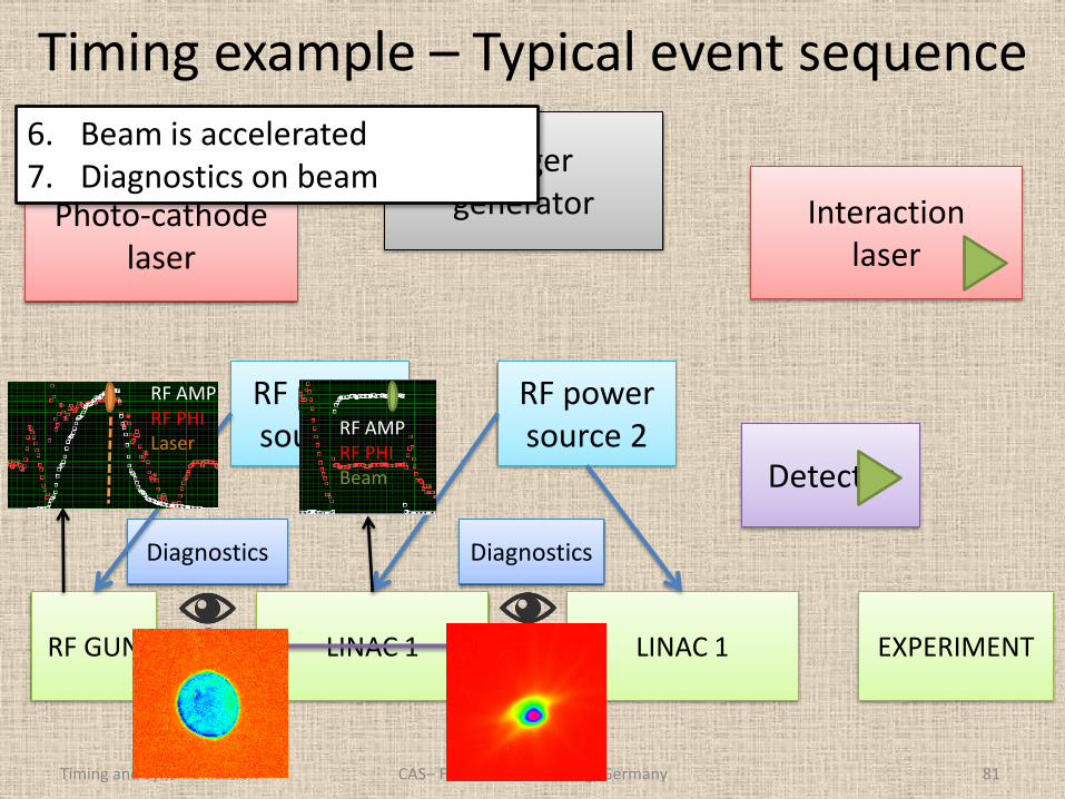
Timing example – Typical event sequence
Timing and Synchronization CAS– FEL & ERL – Hamburg, Germany 81
Photo-cathode laser
Trigger generator
RF GUN LINAC 1 EXPERIMENT LINAC 1
Detector
RF power source 1
RF power source 2
Interaction laser
RF AMP RF PHI Laser
RF AMP RF PHI Beam
6. Beam is accelerated 7. Diagnostics on beam
Diagnostics Diagnostics
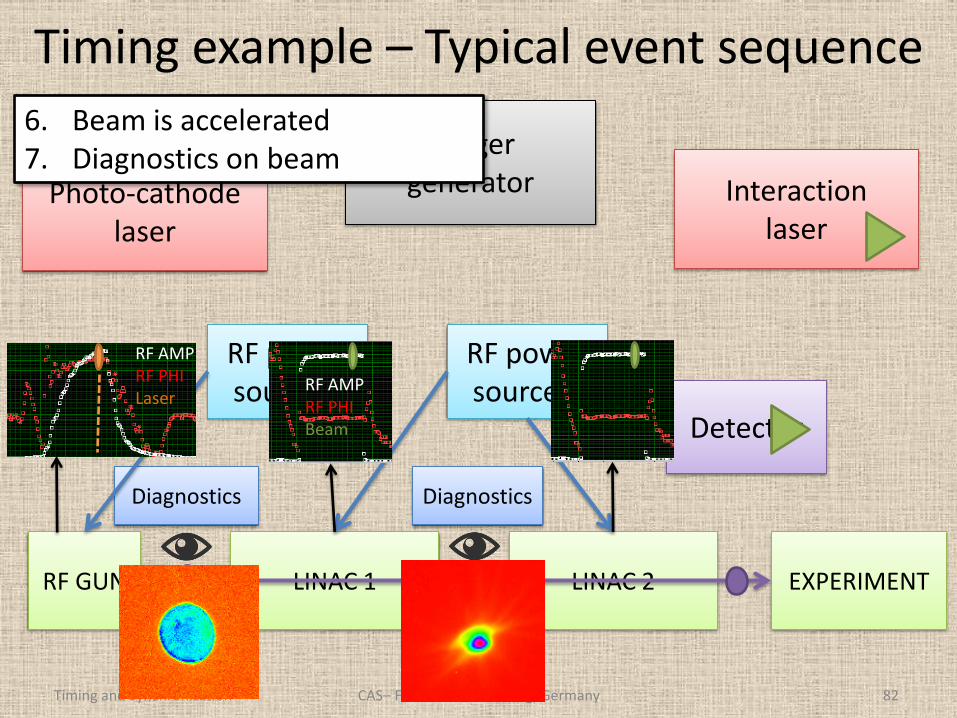
Timing example – Typical event sequence
Timing and Synchronization CAS– FEL & ERL – Hamburg, Germany 82
Photo-cathode laser
Trigger generator
RF GUN LINAC 1 EXPERIMENT LINAC 2
Detector
RF power source 1
RF power source 2
Interaction laser
RF AMP RF PHI Laser
RF AMP RF PHI Beam
6. Beam is accelerated 7. Diagnostics on beam
Diagnostics Diagnostics
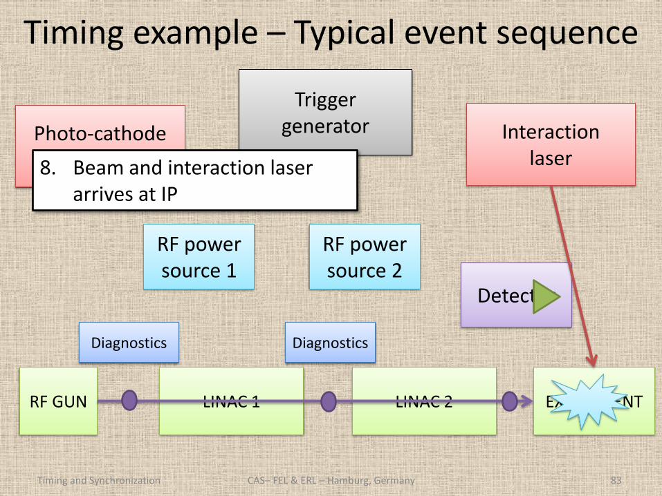
Timing example – Typical event sequence
Timing and Synchronization CAS– FEL & ERL – Hamburg, Germany 83
Photo-cathode laser
Trigger generator
RF GUN LINAC 1 EXPERIMENT LINAC 2
Detector
RF power source 1
RF power source 2
Interaction laser 8. Beam and interaction laser
arrives at IP
Diagnostics Diagnostics
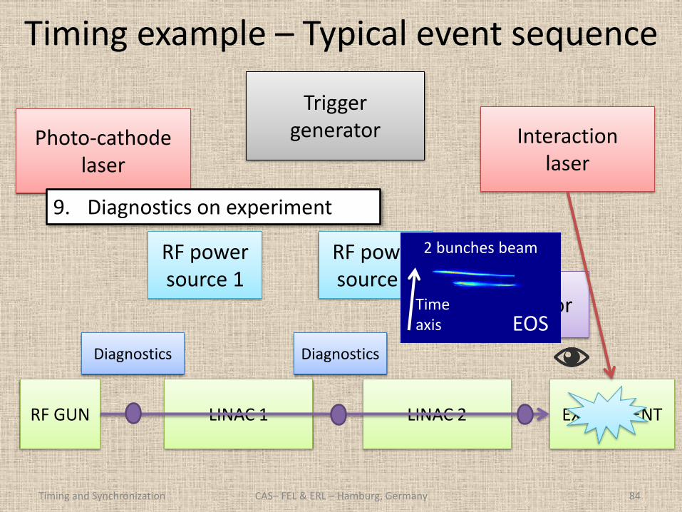
Timing example – Typical event sequence
Timing and Synchronization CAS– FEL & ERL – Hamburg, Germany 84
Photo-cathode laser
Trigger generator
RF GUN LINAC 1 EXPERIMENT LINAC 2
Detector
RF power source 1
RF power source 2
Interaction laser
2 bunches beam
EOS Time axis
9. Diagnostics on experiment
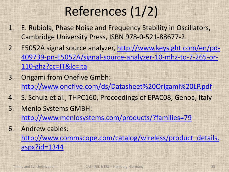
References (1/2)
Timing and Synchronization 85
1. E. Rubiola, Phase Noise and Frequency Stability in Oscillators, Cambridge University Press, ISBN 978-0-521-88677-2
2. E5052A signal source analyzer, http://www.keysight.com/en/pd-409739-pn-E5052A/signal-source-analyzer-10-mhz-to-7-265-or-110-ghz?cc=IT&lc=ita
3. Origami from Onefive Gmbh: http://www.onefive.com/ds/Datasheet%20Origami%20LP.pdf
4. S. Schulz et al., THPC160, Proceedings of EPAC08, Genoa, Italy
5. Menlo Systems GMBH: http://www.menlosystems.com/products/?families=79
6. Andrew cables: http://www.commscope.com/catalog/wireless/product_details.aspx?id=1344
CAS– FEL & ERL – Hamburg, Germany
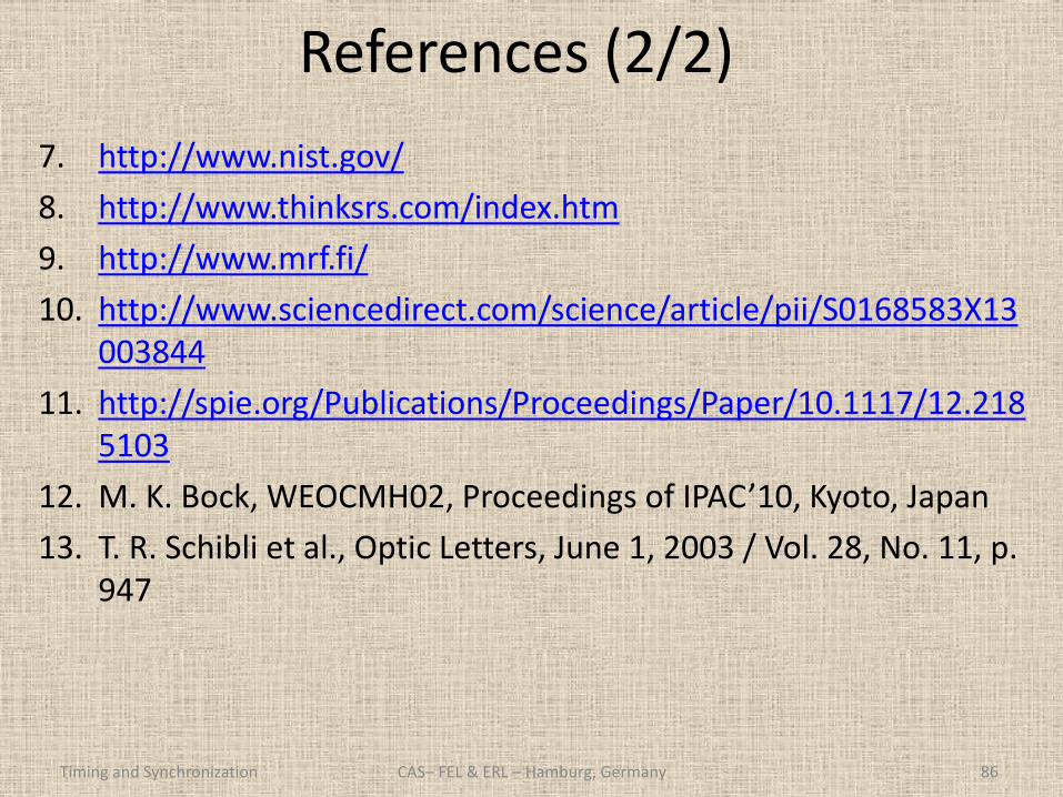
References (2/2)
Timing and Synchronization 86
7. http://www.nist.gov/
8. http://www.thinksrs.com/index.htm
9. http://www.mrf.fi/
10. http://www.sciencedirect.com/science/article/pii/S0168583X13003844
11. http://spie.org/Publications/Proceedings/Paper/10.1117/12.2185103
12. M. K. Bock, WEOCMH02, Proceedings of IPAC’10, Kyoto, Japan
13. T. R. Schibli et al., Optic Letters, June 1, 2003 / Vol. 28, No. 11, p. 947
CAS– FEL & ERL – Hamburg, Germany