Questor Surveys LiOuestor House. 200 Grand River Ave. Brantford. Onta™

II l II11 BII li l — . -. —. --52Heesw88B2 2.12794 WABIKON LAKE 010

INTERPRETATION REPORT

INPUT MARK VI ELECTROMAGNETIC/

MAGNETIC SURVEY

CUMBERLAND RESOURCES LTD.

PROJECT #88032 FEBRUARY 1989

H l II111H II l III "l 111 •"•••" ' " "" "' 1- C O N T 52H86SW8BIB2 2.12794 WABIKON LAKE 010C

1. INTRODUCTION . . . . . . . . . . . . . . . . . . . . . . . . . . . . . . . . . . . . . . . . . . . . . l

2. PROJECT LOCATION . . . . . . . . . . . . . . . . .. . . .. . . . . . . . . . .......... 2

3. SURVEY OPERATIONS . . . . . . . . . . . . . . . . . . . . .. . . .. . . ........... 3

3a. Survey Personnel ................. ................... 33b. Instruments .................... .. . .. ...... ..... .. ... 33c. Production ........ .......... .. .... ...... ............ 43d. Products . . . . .. . . . .. .. . . . . . . . . . . .. . . . .. . . . .... ... . . .. 53e. Survey Procedure ....... ...... ............... .... . ... 53f. Magnetic Diurnal ........ ... . .. .. .. ... . ..... .... ..... 6

4. DATA COMPILATION .. . .. . . . . . . . . . . . . . . . . . . . . . . . . . . . . . . . . . . . . 8

4a. Data Recovery ... .. .. .. . .. ... ... .. .. ..... .... . .... ... 84b. Computer Processing .. .. .. ... ..... . .... .. .. ...... .... 9

5. ELECTROMAGNETIC DATA PRESENTATION . . . . . . . . . . . . . . . . . . . . . . . 11

6. INTERPRETATION GENERAL . . . . . . . . . . . . . . . . . . . . . . . . . . . . . . . . . . . 15

6a. Geological Perspective ...... ... .. .. .. . ... .. ..... .... 156b. Conductivity Analysis .. .......... . . . ..... .... . ... ... 16

l . ELECTROMAGNETIC INTERPRETATION . . . . . . . . . . . . . . . . . . . . . . . . . . . 19

8. CONCLUSIONS AND RECOMMENDATIONS . . . . . . . . . .. . . . .. . . . . . . . . . . 24

APPENDICES

APPENDIX A QUESTOR MARK VI INPUT(R) Systeni . . . . . . . . . . . . . . . A-l

APPENDIX B The Survey Aircraft ....... . . . ... . . . . . . . . .. . . .. B-lAPPENDIX C INPUT System Characteristics .................. C-lAPPENDIX D INPUT Processing . . ... ..... . .. .. .. . .... .... . ... D-lAPPENDIX E INPUT Interpretation Procedures .. .... ...... . .. E-lAPPENDIX F INPUT Response Models . . . . . . . . . . . . . . . . . . . . . . . . . F-lAPPENDIX G Quantitative Interpretation .. ... . .. . ..... .. . .. G-lAPPENDIX H Bibliography .... . . ........ . . . .. . . . . .. . .... . ... H-1

Data Sheets

1. INTRODUCTION

This report details the operation and interpretation of a

fixed-wing airborne time domain electromagnetic and magnetic

survey flown for Cumberland Resources Ltd. (Cumberland). The

system used was the Questor MK VI, 2 ms, system. The standard

specifications for the transmitter and receiver are outlined in

Appendix A.

The survey was commissioned by W. Mccrindle of Cumberland

on December 20, 1988. Philip Salib, Manager, Geophysics for

Questor, supervised the data compilation and interpretation

through to the completion of the project in February, 1989.

The survey objective is the detection and location of base

metal sulphide conductors as well as any structures and

conductivity patterns which could have a positive influence on

gold and base metal exploration.

The primary survey area consists of 417.0 kilometres of

traverse and control lines. These were flown between the dates of

Jan. 17 and Jan. 22 using Thunder Bay as the survey operations

base.

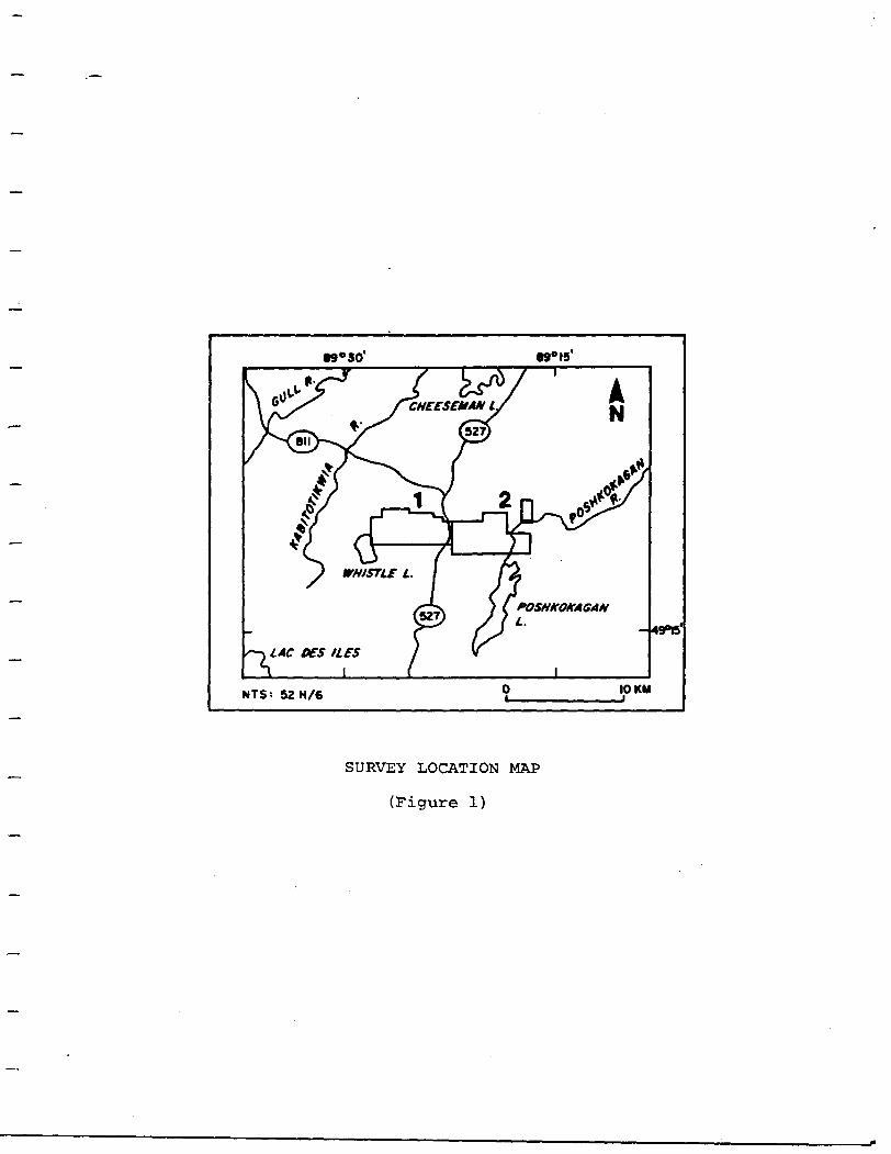
2. PROJECT LOCATION

The survey area lies within the Province of Ontario,

approximately 70 kilometres north-east of the city of Thunder Bay,

The area is located between latitudes 49" 18'N and 49 0 22'N and

longitudes 89 0 16'W and 89 0 29'W (Figure 1). Map sheet Nipigon

(N.T.S. 52H) includes the survey site.

-2-

-49*5'

, LAC DES ILES

NTS: 52H/6 10 KM

SURVEY LOCATION MAP

(Figure 1)

3. SURVEY OPERATIONS

3a. Survey Personnel

The survey crew was made up of experienced Questor

employees:

Crew Manager/Data Technician - R. McDonald

Pilot/Captain of Aircraft - C. Flamand

Co-pilot/Navigator - T. Regehr

Equipment Technician - W. Hutchinson

Aircraft Engineer - T. Kunica

The flight path recovery was completed at the survey base,

while the final data compilation and drafting was carried out by

Questor at its main office. The magnetic and electromagnetic

processing was carried out using Data Plotting software. The

electromagnetic interpretation and report was completed by

Philip Salib.

3b. Instruments

A shorts skyvan, C-GDRG, equipped with the following

instruments was used for the survey:

1. Mark VI Electromagnetic System;

2. Geometrics G-813 Proton Magnetometer (0.1 nT sensitivity);

3. Sonotek SDS 1200 Data Acquisition System;

4. RMS GR33 Analogue Recorder;

5. 35mm Camera, Intervalometer and Fiducial System;

6. Sperry Radar Altimeter.

-3-

A Geometrics G-826 Base Magnetometer was used to monitor

the diurnal magnetic changes.

The equipment, such as the electromagnetic system,

magnetometer and radar altimeter were regularly calibrated at the

beginning and end of each survey flight as well as in mid-flight,

whenever necessary. Details of the calibration procedures are

given in Appendix C.

The continuous chart speed of the RMS recorder was set at

15 cm./minute.

3c. Production

The flight line spacing over the block was 100 metres.

Table l summarizes the kilometres flown during the survey

operation as well as the line direction.

Table l

Traverse lines . . . .. . . .. . . . . . . . . 391.0 km.

Control lines . . .... .. ... ... . . .. 26.0 km.

Total lines . . .. . . ... . . . . . . 417.0 km.

Line direction . . . . . . . . . . . . . . . . . North-South

The survey was completed in three production flights. Four

days were lost during the survey due to bad weather and magnetic

storms.

-4-

3d. Products

The products delivered by Questor to Cumberland Resources

Ltd., together with two copies of the report:

1. Two unscreened master photo mosaic, scale 1:10,000;

2. Two overlays with electromagnetic and magnetometer information

and interpretation shown thereon, scale 1:10,000;

3. Two magnetics overlay, scale 1:10,000;

4. Two composite white prints of (1) S (2);

5. Two composite white prints of (1) S, ( 3);

6. The negative of the flight path film;

7. The flight logs;

3e. Survey Procedure

During the survey, the aircraft maintained a terrain

clearance as close to 122 metres as possible, with the receiver

coil (bird) at approximately 55 metres above the ground surface.

In areas of substantial topographic relief and large population,

the aircraft height may exceed 122 metres for safety reasons. The

height of the bird above the ground is also influenced by the

aircraft's air speed (see Figure CI in Appendix C), which was

maintained at 110 to 120 knots, while on survey.

Whenever possible, the traverse lines were flown in

alternate flight directions (e.g. north then south) to facilitate

the interpretation of dipping conductors. When the traverse line

spacing exceeded twice the normal spacing interval over a 3.0

kilometre distance, the gap is normally filled with an

appropriately spaced fill-in line at a later date.

-5-

The details of each production flight are documented on the

flight logs by the equipment technician. The logs include the

survey times, line numbers and fiducial intervals, as well as a

record of equipment irregularities and atmospheric conditions.

One may refer to them to correlate the flight path film to the

geophysical data.

During the course of the survey the following data were

recorded:

1. Electromagnetic results represented by twelve channels of

successively increasing time delays after cessation of the

exciting pulse (Appendix A);

2. a record of the terrain clearance as provided by radar

altimeter;

3. a photographic record of the terrain passing below the

aircraft as obtained from a 35 mm. camera;

4. time markers impressed synchronously on the.photographic and

geophysical records to facilitate accurate positioning on

photomosaics;

5. airborne magnetometer data;

6. ground base magnetometer station data.

3f. Magnetic Diurnal

Diurnal variations in the earth's magnetic field had been

recorded to an accuracy of ^ l nT using a base station equipped

with a Geometrics G-826 Proton Precession Magnetometer. It was

monitored periodically during the day for severe diurnal changes

(magnetic storms). A variation of 20 nT over a 5 minute time

-6-

period was considered to be a magnetic storm. During such an

event, the survey would normally have been discontinued or

postponed and the survey data would have been reflown.

The base station magnetometer was set up at Thunder Bay.

4. DATA COMPILATION

4a. Data Recovery

The flight path of the aircraft is recorded by a strip

camera on black and white (125ASA, 35 mm.) film which is exposed

continuously during flight at a rate of 5 mm./sec. The apperture

setting on the camera can be manually adjusted by the operator

during flight, assuring the proper exposure of the film. The

camera is fitted with a wide angle 18 mm. lens. Fiducial numbers

are imprinted on the film, marked onto the analogue records and

recorded digitally at the same instant.

The flight line headings are opposite on adjacent lines,

which are normally flown sequentially in an "S" pattern. The

navigation references are flight strips at a scale of 1:10,000

which are made from the base maps. The equipment operator enters

the flight details information into the digital data system which

are recorded and verified (read-after-write). The information

includes line number, time, fiducial range and other pertinent

flight information. This information is compared to the film,

analogue records and the magnetic base station recording at the

completion of the survey flight.

The film and all records are developed, edited and checked

at the completion of each flight. Recovery of the flight track is

carried out by comparing the negative of the 35 mm. film to the

topographic features of the base map. Coincident features are

picked and plotted on exact copies of the stable mosaic base map

on which the final results are drafted. Points are picked at an

average interval of l kilometre. This corresponds to one whole

-8-

fiducial unit or 20 seconds (the picked points will not

necessarily fall on whole fiducial numbers, but on the final

presentation, only the first and last whole fiducial numbers on a

line are marked on each flight line. By interpolation, the whole

numbers are marked as ticks along the flight path).

These procedures are performed on the survey site daily by

the data technician so that the data quality and progress may be

measured objectively. Reflights for covering navigational gaps

and other deficiencies are usually flown on the following day.

The analogue records are inspected for coherence with

specifications, and anomalies are selected for classification and

plotting. Selected anomalous conductors are positioned by

plotting their fiducial positions less the lag factor (Appendix

C). These resultant positions are located by interpolating

between fiducial points established by the flight path recovery

process.

The survey results are presented as an electromagnetic

anomaly map with interpretation and a magnetic contour overlay.

The following chapters describe the interpretation of the

electromagnetic results and present recommendations for ground

follow-up surveys.

4b. Computer Processing

The completed flight path is accurately digitized on a

flat-bed digitizer at Data Plotting using the picked point

co-ordinates. The recovery is then routinely verified by a

computer programme 'speed check 1 , which flags any abnormalities in

-9-

the distance per 5r*tducial unit between picked points on a traverse

line. As a final check, the rough magnetic contour maps are

examined for contour irregularities that could be attributed to

recovery errors.

-10-

5. ELECTROMAGNETIC DATA PRESENTATION

The base maps for the survey area are photomosaics

constructed from 1:15,529 air photographs supplied by Ontario

Ministry of Natural Resources and taken in 1985. The photomosaic

was used to construct the navigation flight strips and also the

base onto which the flight path was recovered. The mosaics are

semicontrolled at a scale of 1:10/000.

The electromagnetic anomaly map presents the information

extracted from the analogue records. This consists chiefly of the

peak anomaly positions and response characteristics, surficial

responses, up-dip responses, and magnetic anomaly locations. In

effect, these represent the primary data analysis. The symbols

are explained in the map legend, but the following observations

are presented:

position of peak anomaly;

conductance or conductivity-thickness;

amplitude of channel 4 response;

position and peak amplitude of associated magnetic anomalies;

where present, surficial, up-dip and poorly defined responses

have been identified with a unique symbol.

The interpretation maps outline the geophysical-geological

interpretation of the electromagnetic, magnetic, geological and

physiographic data. Bedrock conductors have axis locations and

dip directions, when they are interpretable. The anomalous zones

which are recommended for follow-up have a reference label

assigned, to which additional comments and recommendations are

-11-

directed in the Interpretation Section of this report. Surficial

response sources, if any, are mapped out by boundaries showing

their interpreted lateral extent. The following list summarizes

the interpretation presentation:

bedrock conductor axis, probable and possible;

conductor dip;

surficial conductor outlines;

anomalous conductors selected for ground evaluation with

reference number.

The survey results can be classified into the following

categories and are represented on the accompanying interpretation

maps by symbols described below:

a) bedrock conductors - solid axes;

b) weak bedrock conductors - dashed axes;

c) surficial conductors.

Formational Conductors:

Bedrock conductors due to formational horizons are

distinguished by aligned electromagnetic responses in long linear

conductors. These formational conductors form marker horizons

which may be of exploration interest.

-12-

Surficial Conductors:

Broad, low and high amplitude responses which have direct

correlation with lakes, rivers on the survey photomosaic have been

detected. The symbol "S" and the diamond shape on the interpreta

tion map designates this type of conductor which is generally due

to surficial material. These conductors often have low conduct

ances, l to 6 channel responses, shapes, and peak positions can be

matched to the model in Appendix F. In addition, the transient

decays are typical of horizontal lying conductive sources. Often

the longer (elongated) axes of the surficial bodies have no

correlation with magnetics or other regional conductive trends.

Where there is some doubt concerning the possibility of a bedrock

conductor response superimposed on the surficial, these responses

have been plotted with a "poorly defined" symbol.

Some of our selective criteria for the proposed zones are:

- isolated horizon or offset from formational conductors;

- conductivity increase;

- presence of structural features;

- magnetic correlation.

Follow-up recommendations for the formational targets

should be based on favourable geology and previous drilling

results. The stronger, long conductors were often the subject of

earlier geophysical surveys and are well documented. The absence

-13-

of "anomalous" or improved segments along formational horizons is

probably the normal reason for no specific follow-up recommenda

tion in our interpretation.

-14-

6. INTERPRETATION GENERAL

6a. Geological Perspective

The survey area is located northeast of Whistle Lake,

Ontario. It is formed mainly of intrusive diabase (sills and

dykes) of the Keweenawan age. West of Wabikon Lake, Acid Igneous

and metamorphic rocks of Archean age form a 2 kilometres wide band

which extends north-south. These consist mainly of granite

(gneiss), porphyritic granite (gneiss), quartz and feldspar

porphyries, migmatites, syenite, pigmatite, etc. The northwest

corner of the survey area is formed of Basic and intermediate

undifferentiated metavolcanics. Metasedimentary rocks (Arkose,

greywacke, slate mica schists and gneisses) are mapped across the

central section of Lever Lake.

The area geology is similar to Lac Des Mille Lacs' and

the Atikokan areas which are sites of known gold occurrences.

In the Atikokan area, three general types of gold

mineralization are recognized - These are:

i) Marmion Lake Batholith type - quartz veins within shear

zones associated with northeast trending lineaments in the

batholith.

ii) Contact zone type - quartz-carbonate veins within narrow

shear zones located at or near the contacts of batholiths

and metavolcanic belts.

iii) Metavolcanic - hosted strata bound type - concordant lenses

of chert or carbonate with quartz - carbonate veins, hosted

by metavolcanics.

-15-

Since the area geology is similar to the Atikokan area, we

expect a similarity between these two areas in terms of gold

occurrences.

Bibliography:

Pye, E. G. and Fenwick, K.G.; Preliminary Geological Map No.

P.187 (Lac Des Isles Sheet District of Thunder Bay); Ontario

Department of Mines - 1963.

Wilkinson, S. J.; Gold Deposits of the Atikokan Area; Ontario

Ministry of Natural Resources - 1982.

6b. Conductivity Analysis

The conductivity-thickness products of planar horizontal,

and thin steeply dipping conductors are proportional to the time

constant of the secondary field electromagnetic transient decay.

This transient may be closely approximated by an exponential

function for which the conductivity-thickness product is inversely

proportional to the log of the difference of two channel

amplitudes at their respective sample times.

These response functions are presented in the form of

graphs in which the amplitudes of 6 channels of the electro

magnetic response are plotted on a logarithmic scale against

conductivity. The relative amplitudes of the secondary response,

at any given conductivity, may be accurately related to the depth

of a conductor below the surface. These are typically referred to

as Palacky nomog'rams. These are available for a number of

-16-

conductor geometries. It has been found that the shape of the

decay transient and its amplitude is usually unique to a

particular geometry. Therefore, a good "fit" of the peak response

amplitude to one nomogram will define its origin.

The 90 0 nomogram was utilized exclusively to determine the

apparent conductances of the responses obtained from the survey.

This procedure is valid for near vertical conductors, within a dip

range of 45-135 0 , relative to the aircraft flight direction.

Although the conductor depth can be interpreted from

nomograms, the short strike lengths and the variability of

conductor geometry may result in the over-estimation of depths.

The INPUT system depth capability is well characterized for a

vertical plate which is 200 metres deep with a strike length of

600 metres and 300 metres depth extent. The effective penetration

depth increases for a dipping target and decreases for a smaller

size conductor.

Depths were only determined for responses which appear to

fit the interpretation model - a thin near vertical plate with a

strike length of greater than 500 metres. Qualifications for

these determinations are summarized in the interpretation section.

The depths for 10 and 12 channel anomalies were corrected

for the interpreted conductor strike intersection relative to the

line direction and the effects of aircraft altitude deviations

from a flight altitude of 120 metres.

An anomaly listing at the back of this report summarizes

each anomalous response in a numerical sequence. In addition to

the standard anomaly parameters, an "anomaly type" classification

-17-

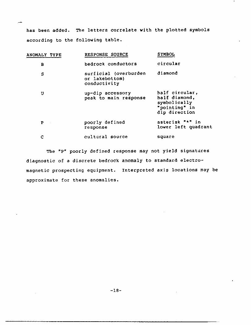
has been added. The letters correlate with the plotted symbols

according to the following table.

ANOMALY TYPE

B

S

U

RESPONSE SOURCE

bedrock conductors

surficial (overburden or lakebottom) conductivity

up-dip accessory peak to main response

poorly defined response

cultural source

SYMBOL

circular

diamond

half circular, half diamond, symbolically "pointing" in dip direction

asterisk "*" in lower left quadrant

square

The "P" poorly defined response may not yield signatures

diagnostic of a discrete bedrock anomaly to standard electro

magnetic prospecting equipment. Interpreted axis locations may be

approximate for these anomalies.

-18-

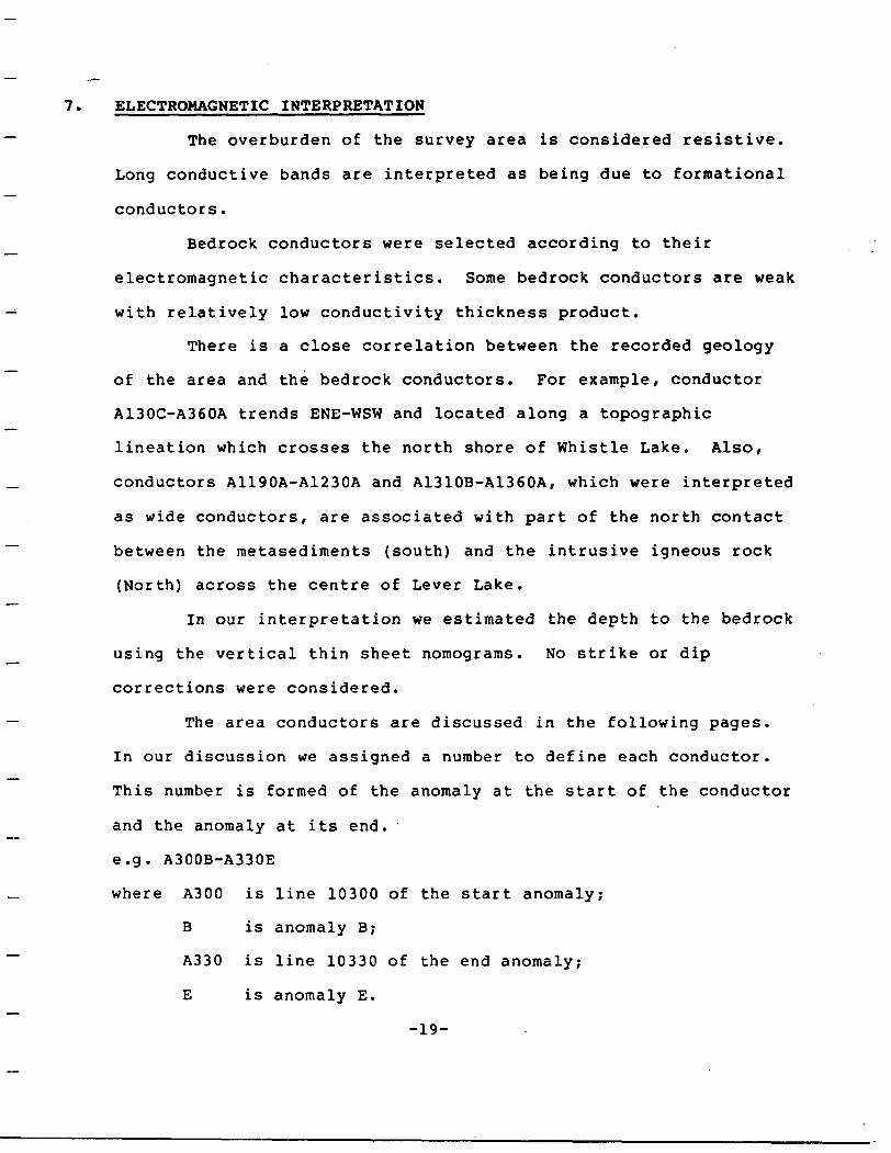
7. ELECTROMAGNETIC INTERPRETATION

The overburden of the survey area is considered resistive.

Long conductive bands are interpreted as being due to forraational

conductors.

Bedrock conductors were selected according to their

electromagnetic characteristics. Some bedrock conductors are weak

with relatively low conductivity thickness product.

There is a close correlation between the recorded geology

of the area and the bedrock conductors. For example, conductor

A130C-A360A trends ENE-WSW and located along a topographic

lineation which crosses the north shore of Whistle Lake. Also,

conductors A1190A-A1230A and A1310B-A1360A, which were interpreted

as wide conductors, are associated with part of the north contact

between the metasediments (south) and the intrusive igneous rock

(North) across the centre of Lever Lake.

In our interpretation we estimated the depth to the bedrock

using the vertical thin sheet nomograms. No strike or dip

corrections were considered.

The area conductors are discussed in the following pages.

In our discussion we assigned a number to define each conductor.

This number is formed of the anomaly at the start of the conductor

and the anomaly at its end.

e.g. A300B-A330E

where A300 is line 10300 of the start anomaly;

B is anomaly B;

A330 is line 10330 of the end anomaly;

E is anomaly E.

-19-

1. Conductor A130C-A360A is a wide bedrock conductive body. It is

associated with a magnetic high. The conductor's strike length is

2400 metres. It is classified as a moderate priority target.

2. Conductor A90A-A160A is distinguished by its short strike length

(800 metres). It has a well defined twelve channel response with

a high conductivity thickness product. The conductor A90A-A160A

is interpreted as wide conductive zone and is given a high t

priority.

3. Conductor A300B-A330E is a short striking wide bedrock conductor.

The conductor is located in a small cleared area. The character

istics of the response are similar to conductor 2 but at a larger

depth. Ground verification should be considered especially at

response 10300B and 10320A. It is classified as a high priority

target.

4. Conductor A20A-A90B is a thin bedrock conductive zone which

strikes east-west. It is associated with a magnetic high. The

conductor should be ground evaluated and is considered as a high

priority target.

5. Conductor A90C-A540A is interpreted as a long formational bedrock

conductor. Its conductivity thickness product varies between 21

and 38 Siemens. The conductor is associated with a magnetic high.

Anomalies 10070B, 10090B, 10250A, 10260D, 10270B, 10340B and

10460C should be ground checked and verified. The zone is

-20-

considered as a moderate priority target. A second weak bedrock

conductor is located 200 metres north of A90C-A540A with parallel

strike direction and displays similar characteristics.

6. Conductor A750A-A760B is a short striking poor bedrock conductor

which trends northeast-southwest. It is defined by two anomalies

where anomaly 10750A represents a good bedrock conductor. The

calculated depth is estimated as 45 metres.

7. Conductor A840B-A850B is a short striking bedrock conductive zone.

It is defined by three anomalies 10840B, 10850 and 19010B. The

response characteristics of these anomalies are similar to a wide

conductor response. We consider this zone as a moderate priority

conductive body. The calculated depth (30 metres) is considered

to be an under estimate because of the conductor's short strike

length (200 metres) relative to the nomograms strike which is 600

metres.

8. Conductor A840C is a single line conductor which is characterized

by 4 channels response. A ground electromagnetic follow-up survey

is recommended to verify its location and trend. It is classified

as a moderate priority conductor.

9. Conductor zone A940C-A1000B is a wide and weak conductive zone.

The zone is possibly at the contact between the metasediments to

the north and the intrusive igneous rocks to the south. Further

-21-

ground verification is recommended. The conductive zone is

considered as a low priority target.

10. Conductor A870A-A950D is interpreted as a wide conductor which is

characterized by l to 6 channels response. The conductive band

follows a magnetic low. It is considered as a low priority

target. A ground follow-up electromagnetic survey is recommended.

11. Conductor A970D-A9020E is a short striking bedrock conductor which

trends northeast-southwest. Ground electromagnetic survey is

recommended to evaluate its origin. It is considered as a

moderate priority target.

12. Conductor A1061C-A10JJOA is formed of four strong parallel

conductors which have northeast-southwest trend. This conductor

is assocated with magnetic high. These conductors are classified

as high priority targets.

13. Conductor A1080E-A1090C is a northwest-southeast strking

conductive body which is associated with magnetic high. The

anomaly is defined by 12 channels response and is considered a

good bedrock conductor. The conductor is classified as a high

priority target.

14. Conductor A1190A-A1230A is a short and wide bedrock conductor.

The conductor is defined by small rounded peak 12 channel response

along four flight lines. It is associated with magnetic high.

-22-

This conductor is located along the central part of Lever Lake

which may represent the contact between the metasediments and the

Intrusive Igneous rocks. It is interpreted as high priority

target and ground follow-up evaluation is recommended.

15. Conductor A1310B-A1360A is a poorly defined conductor which is

interpreted as short and relatively wide conductor. It is

associated with a magnetic low. The conductor is classified as a

low priority target.

-23-

8. CONCLUSIONS AND RECOMMENDATIONS

On the basis of the results of this survey, ground

follow-up work is recommended for several of the selected targets.

The geological picture for the survey area is not

completely known to us so that the geological-geophysical overview

is not completely possible. It is suggested that a geological

reconnaissance survey be carried out, if not already done, in

order to establish a relationship between each of the bedrock

conductors and the basement rocks.

Combining the latest geological data with a calculated

vertical gradient magnetic and a conductivity map could lead to a

reasonable definition of area structure.

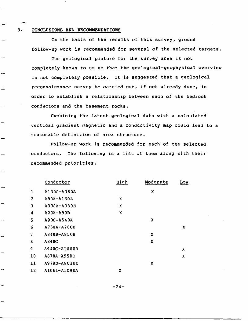
Follow-up work is recommended for each of the selected

conductors. The following is a list of them along with their

recommended priorities.

Conductor High Moderate Low

1 A130C-A360A X

2 A90A-A160A X

3 A300A-A330E X

4 A20A-A90B X

5 A90C-A540A X

6 A750A-A760B X

7 A840B-A850B X

8 A840C X

9 A940C-A1000B X

10 A870A-A950D X

11 A970D-A9020E X

12 A1061-A1090A X

-24-

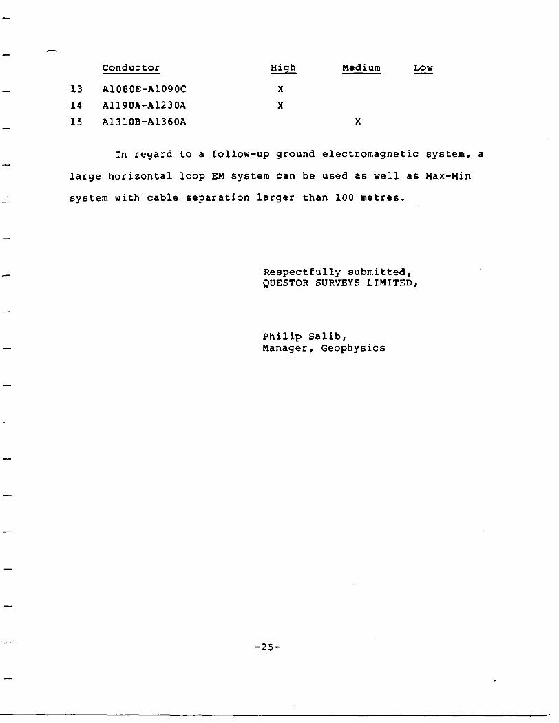
Conductor High Medium Low

13 A1080E-A1090C X

14 A1190A-A1230A X

15 A1310B-A1360A X

In regard to a follow-up ground electromagnetic system, a

large horizontal loop EM system can be used as well as Max-Min

system with cable separation larger than 100 metres.

Respectfully submitted, QUESTOR SURVEYS LIMITED,

Philip Salib, Manager, Geophysics

-25-

APPENDIX A

QUESTOR MARK VI INPUT ( p) AIRBORNE ELECTROMAGNETIC SYSTEM

INPUT (Induced PUlse Transient) is a time domain airborne

electromagnetic survey system( which has been used for over two

million kilonetres of survey, accounting for the majority of all

airborne electromagnetic (A.E.M.) flown world-wide.)

The INPUT apparatus consists of a vertical axis transmitting

loop surrounding the aircraft, a towed 'bird 1 containing a

horizontal axis receiving coil oriented parallel with the direction

of flight, and inboard electronics which control the system timing

as well as performing the required signal processing and recording.

Electric current pulses are applied to the transmitter coil in

alternating polarity directions (Figure A2). The resultant

electromagnetic field induces eddy currents in conducive

terrestrial materials which in turn generate secondary, time

varying, magnetic fields which induce electrical currents in the

receiver coil. The decaying secondary magnetic field is repeatedly

detected and measured by the receiver coil during the intervals

when no current is circulating through the transmitting loop, ie:

in the absence of the primary electromagnetic field. This

measurement technique achieves a high signal-to-noise ratio.

The time-amplitude relationship of the transient secondary

field is controlled by the conductor dimensions, conductivity,

orientation, and position, or distance relative to the INPUT

-Al-

system. Terrestrial materials which have a higher conductivity-

thickness demonstrate a longer secondary field decay persistence.

This physical quality is often associated with massive sulphides as

well as with graphite. In comparison, horizontally layered

surficial conductive materials usually exhibit a more rapid

secondary field decay. A quantitative evaluation of the

conductance of an INPUT anomaly can therefore be made by a

comparison of the associated secondary field decay with an

empirically-derived standard. For purposes of decay-time analysis

and conductance evaluation, the secondary field is sampled over

twelve consecutive and discrete time intervals. The average value

of the secondary field during each of these intervals is averaged

over a number of measurement cycles, and the resultant

running-average value for each time-channel is systematically

recorded in both analogue and digital formats.

-A2-

INPUT System Characteristics

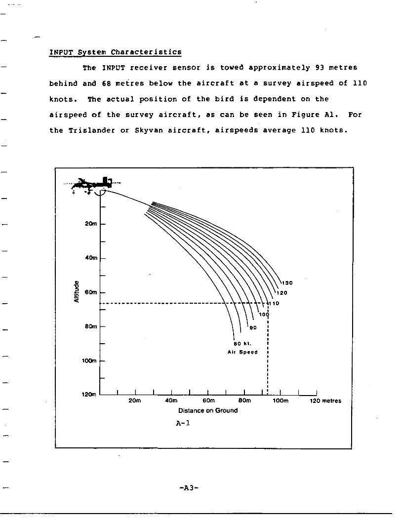
The INPUT receiver sensor is towed approximately 93 metres

behind and 68 metres below the aircraft at a survey airspeed of 110

knots. The actual position of the bird is dependent on the

airspeed o f the survey aircraft, as can be seen in Figure Al. For

the Trislander or Skyvan aircraft, airspeeds average 110 knots.

120m20m 40m 60m 80m

Distance on GroundA-1

100m 120 metres

-A3-

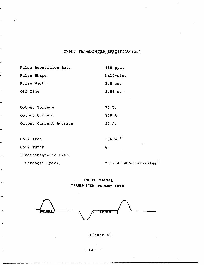
INPUT TRANSMITTER SPECIFICATIONS

Pulse Repetition Rate

Pulse Shape

Pulse Width

Off Time

180 pps.

half-sine

2.0 iris.

3.56 ms .

Output Voltage

Output Current

Output Current Average

75 V.

240 A.

54 A.

Coil Area

Coil Turns

Electromagnetic Field

Strength (peak)

186 m,

6

267,840 amp-turn-meter 2

INPUT SIGNAL TRANSMITTED PRIMARY FIELD

/Figure A2

-A4-

SAM

PLIN

G

OF

INPU

T S

IGN

AL

jjise

c.

L.

O

t

*M

org

—

O

CM

ro

^-

III

CM ro

inID

(D

OD

00

CM

f-

Of-

oj

R! i-(M N (M

l

O

00

(DOD

u)

in

— CM

10

O CM

ID

to O) r-

CM f- cnCM K ro

CM f^ en

Chan

nel

12

34

810

12

Fig

ure

A3

\

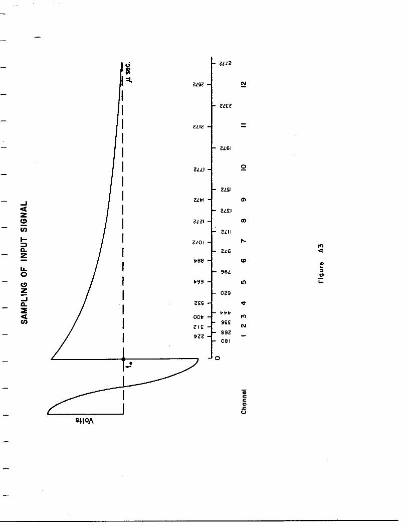
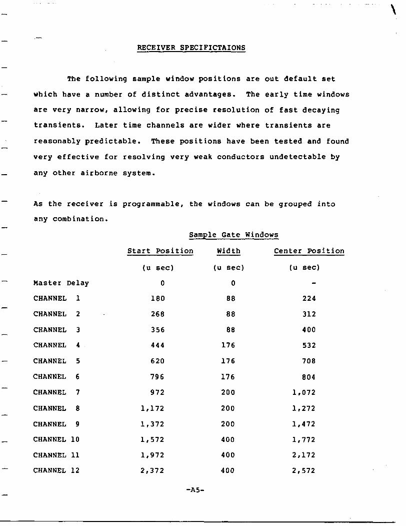
RECEIVER SPECIFICTAIONS

The following sample window positions are out default set

which have a number of distinct advantages. The early time windows

are very narrow, allowing for precise resolution of fast decaying

transients. Later time channels are wider where transients are

reasonably predictable. These positions have been tested and found

very effective for resolving very weak conductors undetectable by

any other airborne system.

As the receiver is programmable, the windows can be grouped into

any combination.

Sample Gate Windows

Master

CHANNEL

CHANNEL

CHANNEL

CHANNEL

CHANNEL

CHANNEL

CHANNEL

CHANNEL

CHANNEL

CHANNEL

CHANNEL

CHANNEL

Delay

1

2

3

4

5

6

7

8

9

10

11

12

Start Position

(u sec)

0

180

268

356

444

620

796

972

1,172

1,372

1,572

1,972

2,372

Width

(u sec)

0

88

88

88

176

176

176

200

200

200

400

400

400

Center Position

(u sec)

-

224

312

400

532

708

804

1,072

1,272

1,472

1,772

2,172

2,572

-A5-

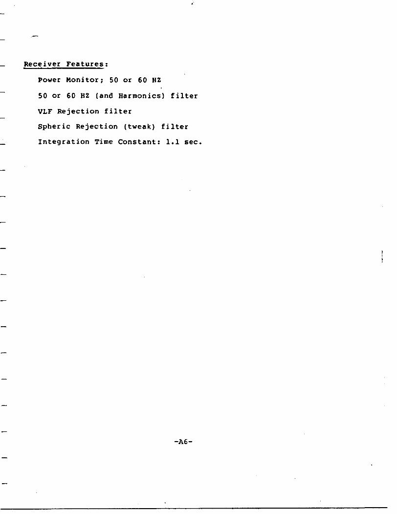
Receiver Features;

Power Monitor; 50 or 60 HZ

50 or 60 HZ (and Harmonics) filter

VLF Rejection filter

Spheric Rejection (tweak) filter

Integration Tine Constant: 1.1 sec.

-A6-

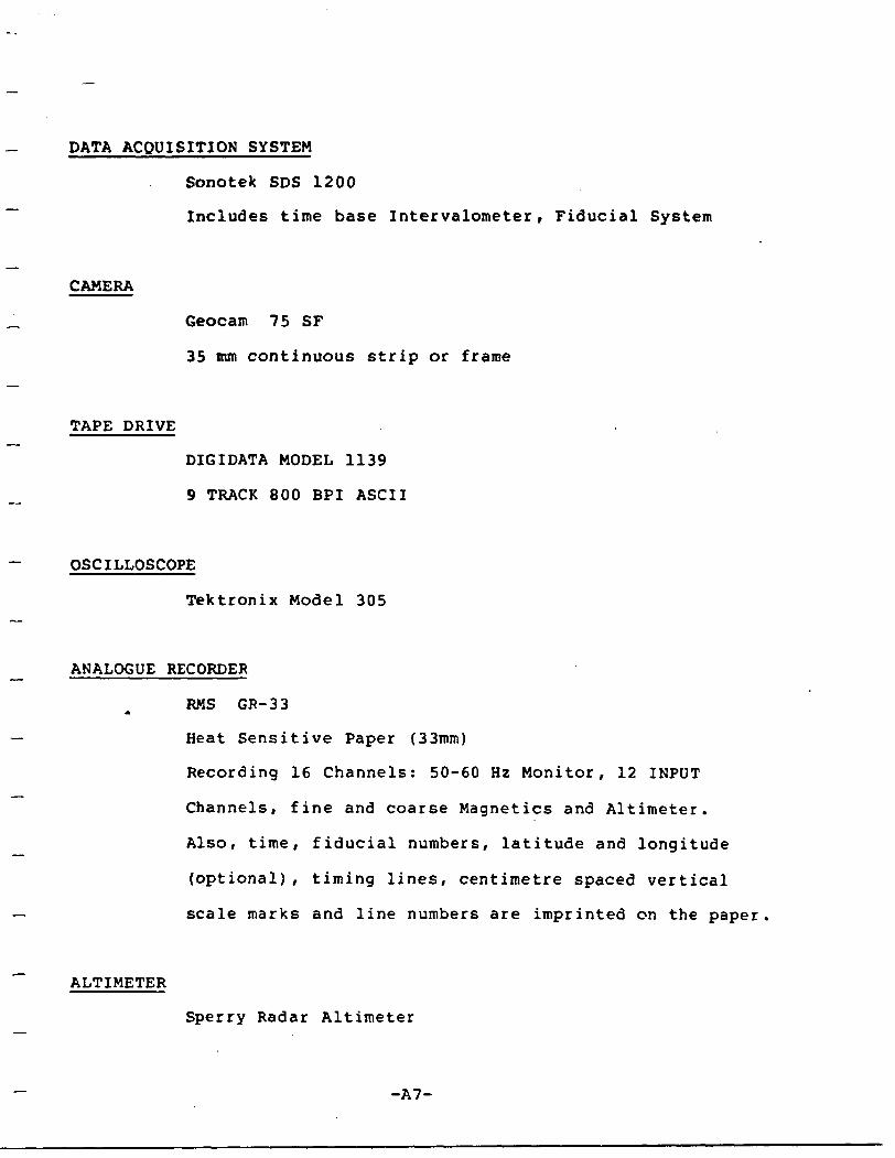
DATA ACQUISITION SYSTEM

Sonotek SDS 1200

Includes time base Intervalometer, Fiducial System

CAMERA

Geocam 75 SF

35 mm continuous strip or frame

TAPE DRIVE

DIGIDATA MODEL 1139

9 TRACK 800 BPI ASCII

OSCILLOSCOPE

Tektronix Model 305

ANALOGUE RECORDER

RMS GR-33

Heat Sensitive Paper (33mm)

Recording 16 Channels: 50-60 Hz Monitor, 12 INPUT

Channels, fine and coarse Magnetics and Altimeter.

Also, time, fiducial numbers, latitude and longitude

(optional), timing lines, centimetre spaced vertical

scale marks and line numbers are imprinted on the paper

ALTIMETER

Sperry Radar Altimeter

-A7-

GEOMETRICS MODEL G-813 PROTON MAGNETOMETER

The airborne magnetometer is a proton free precession sensor

which operates on the principle of nuclear magnetic resonance to

produce a measurement of the total magnetic intensity. It has a

sensitivity of 0.1 nanotesla and an operating range of 17,000

nanoteslas to 95,000 nanoteslas. The G-813 incorporates fully

automatic tuning over its entire range with manual selection of the

ambient field starting point for quick startup. The instrument can

accurately track field changes exceeding 5,000 nT and for this

survey has an absolute accuracy of 0.5 NT at a l second sample

rate. The sensor is a solenoid type, oriented to optimize results

in a low ambient magnetic field. The sensor housing is mounted on

the tip of the nose boom supporting the INPUT transmitter cable

loop. A 3 term compensating coil arrangement and permalloy strips

are adjusted to counteract the effects of permanent and induced

magnetic fields in the aircraft.

Because of the high intensity electromagnetic field produced

by the INPUT transmitter, the magnetometer and INPUT results are

sampled on a time share basis. The magnetometer head is energized

while the transmitter is on, but the read-out is obtained during a

short period when the transmiter is off. Using this technique, the

sensor head is energized for 0.80 seconds and subsequently the

precession frequency is recorded and converted to nanoteslas during

the following 0.20 second when no current pulses are induced into

the transmitter coil.

-A8-

APPENDIX B

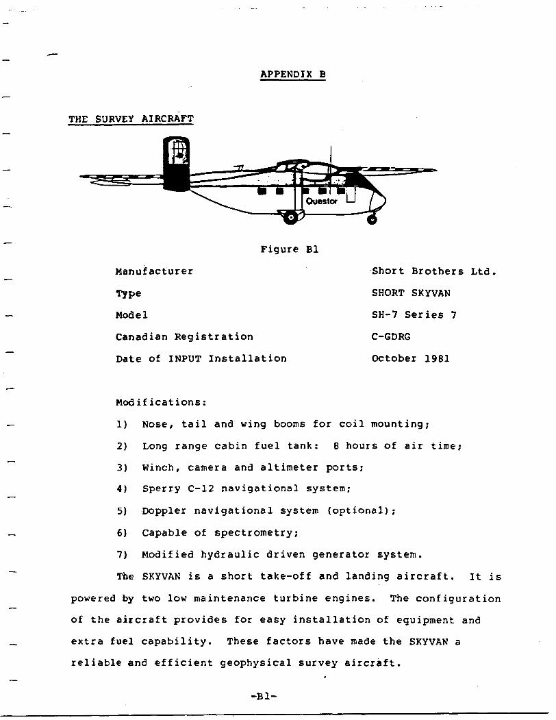
THE SURVEY AIRCRAFT

Figure Bl

Manufacturer

Type

Model

Canadian Registration

Date of INPUT Installation

Short Brothers Ltd

SHORT SK WAN

SH-7 Series 7

C-GDRG

October 1981

Modifications:

1) Nose, tail and wing booms for coil mounting;

2) Long range cabin fuel tank: 8 hours of air tine;

3) Winch, camera and altimeter ports;

4) Sperry C-12 navigational system;

5) Doppler navigational system (optional);

6) Capable of spectrometry;

7) Modified hydraulic driven generator system.

The SKYVAN is a short take-off and landing aircraft. It is

powered by two low maintenance turbine engines. The configuration

of the aircraft provides for easy installation of equipment and

extra fuel capability. These factors have made the SKYVAN a

reliable and efficient geophysical survey aircraft.*

-B l-

APPENDIX C

CALIBRATION OF THE SURVEY EQUIPMENT

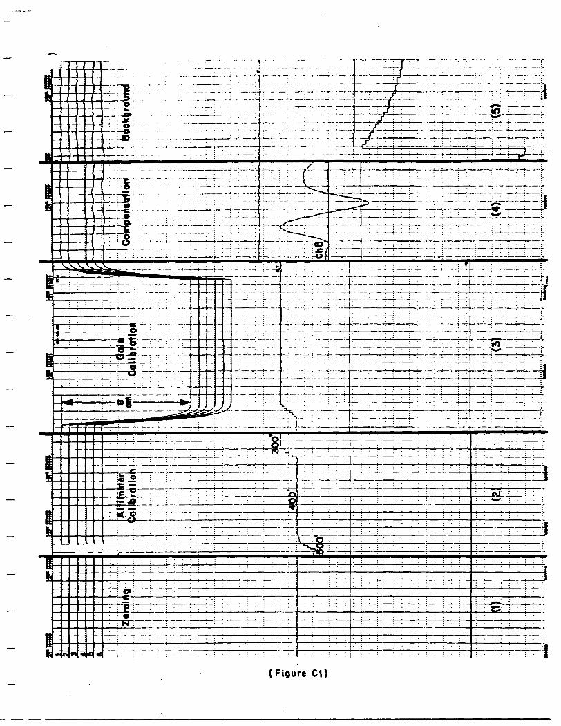
At the beginning of each survey flight, the calibration of

the survey equipment is performed by the following tests:

1) zero the 12 channel levels;

2) altimeter calibration;

3) calibration of INPUT receiver gain;

4) aircraft compensation;

5) record background E.M. levels at 600m.

This sequence of tests are recorded on the analogue records

and may be repeated in midflight given that the duration of the

flight is sufficiently long (Figure CI). At the termination of

every flight, the calibration of the equipment is checked and

recorded for any drift that may have occurred during the flight.

Channels l to 12 are zeroed on the analogue record by first

placing the INPUT receiver into calibration mode, which isolates

the receiver from any bird signal. Then, the channels are adjusted

so that they are evenly spaced 5mm. apart with channel 12

positioned on the first half cm. line at the top of the record.

-CI-

(Figure CI)

The magnetic data is recorded on two scales, a fine and a

coarse scale. The two scales are permanently set so that a full

scale deflection of 100 nanoTeslas is equivalent to 10 cm. on the

fine scale and a shift of 2 cm. indicates a 1000 nanoTesla change

on the coarse scale.

The aircraft altimeter is calibrated so that an altitude of

122 m. is positioned near the 14 cm. line from the bottom of the

analogue record. This is the nominal flying height of INPUT

surveys, wherever relief and aircraft performance are not limiting

factors. A cm. below the 122 m. level corresponds to an altitude

of 153 m. while a cm. above correlates with 91 m. in altitude.

The INPUT receiver gain is expressed in parts per million

of the primary field amplitude at the receiver coil. At the

'bird 1 , the primary field strength is maintained at 1.05 volts

peak. The gain of the receiver is calibrated by introducing a

calibration signal at the input stage of 4.0 mV. This signal

should cause an 8 cm. deflection on all 12 traces, which translates

to a sensitivity of:

((4 x 10" 3 volts/1.05 volts)/8 cm) x 10 6 ppm * 475 ppm/cm

In most towed-receiver airborne E.M. systems, variations in

the position of the receiving coil 'bird 1 in relation to the

aircraft generates a source of noise and needs to be taken account

of before every survey flight is initiated.

-C2-

The noise is the result of spurious eddy currents in the

frame of the aircraft, which have been induced by the primary

electromagnetic field of the INPUT system.

Compensation is the technique by which the effects of the

noise are minimized. A reference signal obtained from the primary

field at the receiver coil is utilized to compensate each channel

of the receiver for coupling differences caused by bird motion

relative to the aircraft. This signal is proportional to the

inverse cube of the distance between the bird and aircraft.

Compensation procedures are carried out at an altitude at

or above 600 metres in order to eliminate the influence of external

geological and cultural noise. Coupling changes are induced by

pitching the aircraft up and down to promote bird motion. The gain

of channel 8 is increased to dramatize the effect of the bird

swing. The compensation circuitry is then appropriately tuned to

minimize the effect of bird motion on the remaining channels.

Phase considerations of channel 8 relative to the other channels

dictates whether sufficient compensation has been applied. If the

channels are in-phase with channel 8 during this procedure, an

over-compensated situation is indicated, whereas, out-of-phase

would be indicative of an under-compensation case.

The background levels of the E.M. channels are recorded at

the 600 metre altitude. They are used to determine the drift that

may occur in the E.M. channels during the progression of a survey

flight. If drift has occurred, the E.M. channels are brought back

to a levelled position by use of the linear interpolation technique

during the data processing.

-C3-

TIME CONSTANT OF THE INPUT SYSTEM

The time constant, is defined as the time for a receiver

signal (voltage) to build up or decay to 63.2% of its final or

initial value. A longer time constant reduces background noise but

also has the effect of reducing the amplitude of a signal as well

as the resolution of the system.

A time constant is periodically verified for continuity. It

can be measured from the exponential rise or decay of the

calibration signal, recorded during the calibration of the receiver

gain (figure CI,(3)}.

-C4-

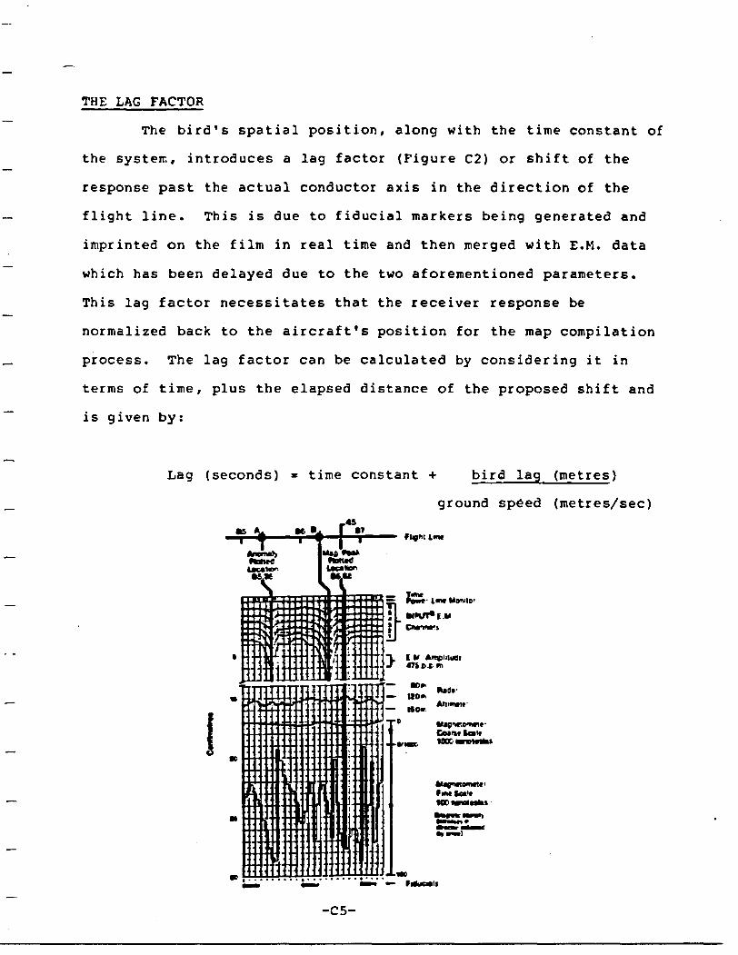
THE LAG FACTOR

The bird's spatial position, along with the time constant of

the system, introduces a lag factor (Figure C2) or shift of the

response past the actual conductor axis in the direction of the

flight line. This is due to fiducial markers being generated and

imprinted on the film in real time and then merged with E.M. data

which has been delayed due to the two aforementioned parameters.

This lag factor necessitates that the receiver response be

normalized back to the aircraft's position for the map compilation

process. The lag factor can be calculated by considering it in

terms of time, plus the elapsed distance of the proposed shift and

is given by:

Lag (seconds) s time constant -t- bird lag (metres)

ground speed (metres/sec)

H

-C5-

The tine constant of the system introduces a 1.1 second lag

while, at an aircraft velocity of 110 knots, the 'bird 1 lag is 1.7

seconds. The total lag factor which is to be applied to the INPUT

E.M. dat at 110 knots is 2.8 seconds (0.14 fiducials). It must be

noted that these two parameters vary within a small range dependent

on the aircraft velocity, though they are applied as constants for

consistency. As such, the removal of this lag factor will not

necessarily position the anomaly peaks directly over the real

conductor axis. The offset of a conductor response peak is a

function of the system and conductor geometry as well as

conductivity.

The magnetic data has a 1.0 second lag factor introduced

relative to the real time fiducial positions. This factor is

software controlled with the magnetic value recorded relative to

the leading edge (left end) of each step 'bar 1 , for both the fine

and coarse scales. For example, a magnetic value positioned at

fiducial 10.00 on the records would be shifted to fiducial 9.95

along the flight path.

A lag factor of 2 seconds (0.10 fiducial) is introduced to

correct 50-60 Hz monitor for the effects of bird position and

signal processing. In cases where a 50-60 Hz signal is induced in

a long formational conductor, a 50-60 Hz secondary electromagnetic

transient may be detected as much as 5 km. from the direct source

over the conductive horizon.

The altimeter data has no lag introduced as it is recorded

in real time relative to the fiducial markings.

-C6-

APPENDIX D

INPUT DATA PROCESSING

The QUESTOR designed and implemented computer software for

automatic interactive compilation and presentation, may be applied

to all QUESTOR INPUT Systems. Although many of the routines are

standard data manipulations such as error detection, editing and

levelling, several innovative routines are also optionally

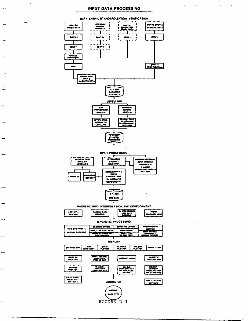
available for the reduction of INPUT data. The flow chart on the

following page (Figure Di) illustrates some of the possibilities.

Software and procedures are constantly under review to take

advantage of new developments and to solve interpretational

problems.

a) INPUT Data Entry and Verification

During the data entry stage, the digital data range is

compared to the analog records and film. The raw data may be

viewed on a high-resolution video graphics screen at any

desirable scale. This technique is especially helpful in the

identification of background level drift and instrument

problems.

b) Levelling Electromagnetic Data

Instrument drift, recognized by viewing compressed data from

several hours of survey flying, is corrected by an inter-active

levelling program. Although only two or three calibration

sequences are normally recorded, levelling can be performed with

any multiple non-anomalous background recordings to divide a

possible problematic situation into segments.

-Di-

INPUT DATA PROCESSING

DATA ENTRY. STANDARDIZATION. VERIFICATION

MPUT PROCESSING

MAGNETIC QUID INTERPOLATION AND DEVELOPMENT•CTMAl E MTA

MAGNETIC PROCESSMG

DISPLAY

MUMCt CUT l HMD con l Hem* j H.CTHK l "^

ARCHIVINO

MTATT*t

FIGURE D l

Each of the 12 INPUT channels are levelled independently. The

sensitivity of the levelling process is normally better than

15 ppr on data with a peak-to-peak noise level of 30 ppm.

c) Data Enhancement

Normal INPUT processing does not include the filtering of

electromagnetic data. The residual high frequency variations

often apparent on analogue INPUT data, are due almost entirely

to atmospheric static discharge "spherics". In conductive

environments, spherics are apparently grounded and effectively

filtered. In resistive environments, frequency spectrum

analysis and subsequent FFT (Fast Fourier Transform) filters

may be applied to data to reduce the noise envelope.

d) Selection of EM Anomalies

E.K. anomalies are normally picked by an automatic anomaly

peak selection program, which also determines the number of

channels for the anomaly. In certain circumstances,

particularly when conductive overburden responses are concerned,

it may be preferable that the anomalies be manually selected.

The E.K. data can be viewed sequentially on a graphic screen

terminal for manual anomaly picking. An anomaly 'type'

classification is ascribed during the manual selection or

entered after the cross-correlation procedure, in the case of

the automatic selection.

-D2-

APPENDIX E

INPUT INTERPRETATION PROCEDURES

In the analysis of INPUT responses, the following parameters

are considered:

a) Anomaly Characteristics

amplitude, number of channels, decay rate, symmetry;

half width and the overall relationships to adjacent and

along strike responses, plus the ground-to-aircraft

distance.

b) Geological Relationships

known geological strike and dip patterns;

host rock, overburden and residual clay conductivity.

c) Cultural Relationships

as directed by the power line monitor;

correlation with known features such as buried

pipelines, fence lines, farm and industrial buildings,

etc.

For each anomaly selected the following are documented:

- line number and anomaly letter;

fiducial location on line;

interpreted source type of the anomaly - bedrock,

surficial, or cultural;

number of channels of response;

- amplitudes in parts-per-million of channels l through

12;

apparent conductance in Siemens based on the appropriate

source model;-El-

corresponding magnetic association in nanoTeslas with

fiducial location;

altitude (ground-to-aircraft) In metres.

From the anomaly characteristics, interpretative aspects

such as up-dip responses, dip direction and altitude are made.

Anomalies are then grouped into linear trends for bedrock

conductors, and zones for horizontal conductivity contrasts, by

correlation with adjacent on-strike responses.

Also, the interpreted source of the INPUT response is

categorized as bedrock, surficial, accessory (up-dip) or cultural.

Bedrock conductors are caused by massive sulphides, graphite

bearing formations, serpentinized peridotites and in some instances

by faults or shear zones. Magnetite concentrations may also, in

some circumstances, yield anomalous INPUT responses. INPUT

responses have been well documented by Macnae (1979), and Palacky

and Sena (1979).

MASSIVE SULPHIDE DEPOSITS

The conductivity characteristic of massive sulphides is due

to intergranular connections forming elongated sheet-like masses

which permit the induction of eddy currents. These produce a

secondary electromagnetic field which can be detected and

quantitatively measured.

In most sulphide bodies the conductivity is caused by

pyrrhotite and chalcopyrite. Pyrite, which often forms the greater

quantity of sulphides present, usually occurs as isolated, albeit

-E2-

closely spaced grains or crystals, and therefore, only produces

moderate or weak responses. Sphalerite does not provide anomalous

responses and can even insulate the better sulphide conductivity

portion of a deposit. The resultant overall conductivity response

from a massive sulphide deposit is in the range of 5 to 30

Siemens/metre, although individual lenses or mineral aggregates may

have much higher conductivities.

Massive sulphide deposits occur as injections, veins and

stratiform bodies of variable size, geometry and conductivity.

Given these variables, there are no universal rules for all

sulphide deposits; however, there are some general observations

regarding the INPUT responses. These are:

Amplitudes primarily increase in response to conductor

strike and depth extent up to an "infinite" size of some

600 metres by 300 metres. Thereafter, source conductor

width contributes to amplitudes, that is, amplitude is

dependant on sulphide mass.

Conductance varies independently with the overall

integrated mineralogy and form of the sulphide

components.

INPUT is often utilized in the search for volcanogenic

copper-zinc sulphide deposits. These deposits are usually

associated with felsic volcanic sequences, often at the interface

of felsic-mafic rocks or with intercalated tuffs and/or sedimentary

rocks. Many of these deposits have stringer sulphide zones in the

footwall rocks related to feeder vent alteration systems and these

can also contribute to the INPUT response. Laterally, the main

-E3-

sulphide deposits can lens out quickly or continue as minor bands,

lenses or disseminated sulphides within nore regionally extensive

coeval tuffs or sediments and also provide INPUT responses along a

considerable strike extent. All these variables must be considered

in the explorationist's depositional model and in the analysis and

interpretation of the geophysical responses. A careful analysis of

the conductances, apparent widths (half peak width) and magnetic

responses will often reveal the geometry-source aspects of the

deposit. Stratiform base metal sulphides of up to 2,000 metres

strike extent are known, although most sizeable deposits have

strike lengths between 500 and 1,000 metres.

The magnetic response of a sulphide deposit is the most

deceiving information available to the explorationist. Although

many large economic deposits have a strong direct magnetic

association, some of the largest base metal deposits have no

magnetic association. Others have flanking magnetic anomalies

caused by pyrrhotite/magnetite deposits in volcanic vent systems

flanking the main sulphide body. Essentially non- homogeneous

conductivities and magnetic responses may be favourable parameters.

GRAPHITIC SEDIMENTARY CONDUCTORS

Graphitic sediments are usually found within the sedimentary

facies of greenstone belts. These represent a low energy,

subaqueous sedimentary environment. Graphites are often located in

basins of the subaqueous environment, producing the same

geometrical shape as sulphide concentrations. Most often however,

they form long, homogeneous planar sequences. These may have

-E4-

thicknesses from a metre to hundreds of metres. The recognition of

graphite in this setting is often straightforward because

conductivities and apparent widths may be very consistent along

strike. Strike lengths of tens of kilometres are common for

individual horizons.

The conductivity of a graphite formation is a function of

two variables:

a) the quality and quantity of the graphite, and

b) the presence of pyrrhotite as an accessory conductive

mineral

Pyrite is the most common sulphide mineral occuring within

graphitic sequences. It does not contribute significantly to the

overall conductivity as it will normally be found as disseminated

crystals. Amphibolite facies metamorphism will often be sufficient

to convert carbonaceous sediments to graphitic beds. Likewise,

pyrite will often be transformed to pyrrhotite.

Without pyrrhotite, most graphitic conductors have less than

10 S conductivity-thickness value as detected by the INPUT system

or l to 10 S/m conductivity from ground geophysical measurements.

With pyrrhotite content, there may be little difference from other

sulphide conductors.

It is not unusual to find local concentrations of sulphides

within graphitic sediments. These may be recognized by local

increases in apparent width, conductivity or as a conductor offset

from the main linear trends.

Graphite has also been noted in fault and shear zones which

may cross geological formations at oblique angles.

-E5-

SERPENTINIZED PERIDOTITES

Serpentinized peridotites are very distinguishable from

other anomalies. Their conductivity is low and is caused partially

by serpentine. They have a fast decay rates, large amplitudes and

strong magnetic correlation. Large profile widths with a shape

similarity to surficial conductors are a common charactreristic.

MAGNETITE

INPUT anomalies over massive magnetites correlate to the

total Fe content. Below 25-3C^ Fe, little or no response is

obtained. However, as the Fe percentage increases, strong

anomalies may result with a rate of decay that usually is more

pronounced than those for massive sulphides.

Negative INPUT responses may occur in a resistive but very

magnetic iron formation, the result of a very high permeability,

however, these are extremely rare.

SURFICIAL CONDUCTORS

Surficial conductors are characterized by fast decay rates

and usually have a conductivity-thickness of 1-5 Siemens. This

value is much higher in saline conditions. Overburden responses

are broad, more so than bedrock conductors. Anomalies due to

surficial conductivity are dependent on flight direction. This

causes a staggering effect from line-to-line as the INPUT response

is much stronger for the leading edge of the flat lying surface

materials than for the trailing edge. When the surficial response

has the form of a thin horizontal ribbon, anomalies may be very

-E6-

difficult to distinguish from weak bedrock conductors. A unique

identification for all geometries of horizontal ribbon, sheet and

layer conductivity contrasts is best accomplished by matching of

transient decay amplitudes to the appropriate response nomogram.

CULTURAL CONDUCTORS

Cultural conductors are identifiable by examining the power

line monitor and the film to locate railway tracks, power lines,

buidings, fences or pipe lines. Power lines produce INPUT

anomalies of high conductivity that are similar to bedrock

responses. The strength of cultural anomalies is dependent on the

grounding of the source. INPUT anomalies usually lag the power

line monitor by l second, which should be consistent from

line-to-line. If this distance between the INPUT response and the

power line monitor differs between lines, then there is the

possibility of an additional conductor present. The amplitude and

conductivity-thickness of anomalies should be consistent from

line-to-line.

-E7-

APPENDIX F

INPUT RESPONSE MODELS

To the interpreter, one of the main advantages of the INPUT

system geometry is the variation of the secondary response with

conductor shape, size, depth and conductivity (Palacky 1976, 1977).

When we discuss the recognition parameters, one of the

variables which is often omitted, is the plotting position of the

main peaks in opposite flight directions on adjacent lines. In

many cases, the responses may appear similar, but the plotting

positions will show significant differences. These situations will

be illustrated in the following section.

A third conductor identification factor is the INPUT decay

transient for the main response peak. The decays may be used to

identify the type of source, independent of the geometrical

response which is dependent on the mutual coupling.

-FI-

MODEL AND PHYSICAL CONDUCTORS

Economic conductive mineral deposits have no unique feature

which would make their identification a straightforward process.

Most ore bodies do have conductivity contrasts and at least one

dimension which is significantly small. A conductivity contrast is

necessary to overcome the "skin depth" attenuation effects of

conductive overburden or lateritic soils on the primary

electromagnetic field (West and Macnae 1982). The recognition of

dipping conductors is possible, mainly due to the double peaks

encountered in an updip flight direction (Figure F4). A horizontal

mineral deposit is potentially the most difficult to select because

the horizontal sheet model also applies to conductive overburden

and lateritic soils. The theoretical shapes may be matched to

physical-geological situations as has been done in the following

summary:

-F2-

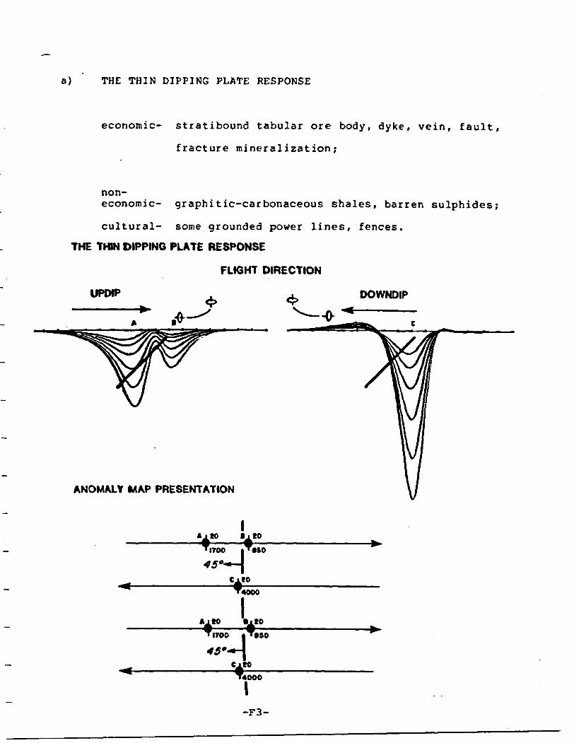
a) THE THIN DIPPING PLATE RESPONSE

economic- stratibound tabular ore body, dyke, vein, fault,

fracture mineralization;

non- economic- graphitic-carbonaceous shales, barren sulphides;

cultural- some grounded power lines, fences.

THE THIN DIPPING PLATE RESPONSE

FLIGHT DIRECTION

UPDIP DOWNDIP

ANOMALY MAP PRESENTATION

-4000

w—30T iroo i Ti

4000

-F3-

The interpreted conductor axis location varies with the

source dip, conductivity, depth* thickness, depth extent and angle

of intersection of the flight line to the conductor (strike

direction).

-F4-

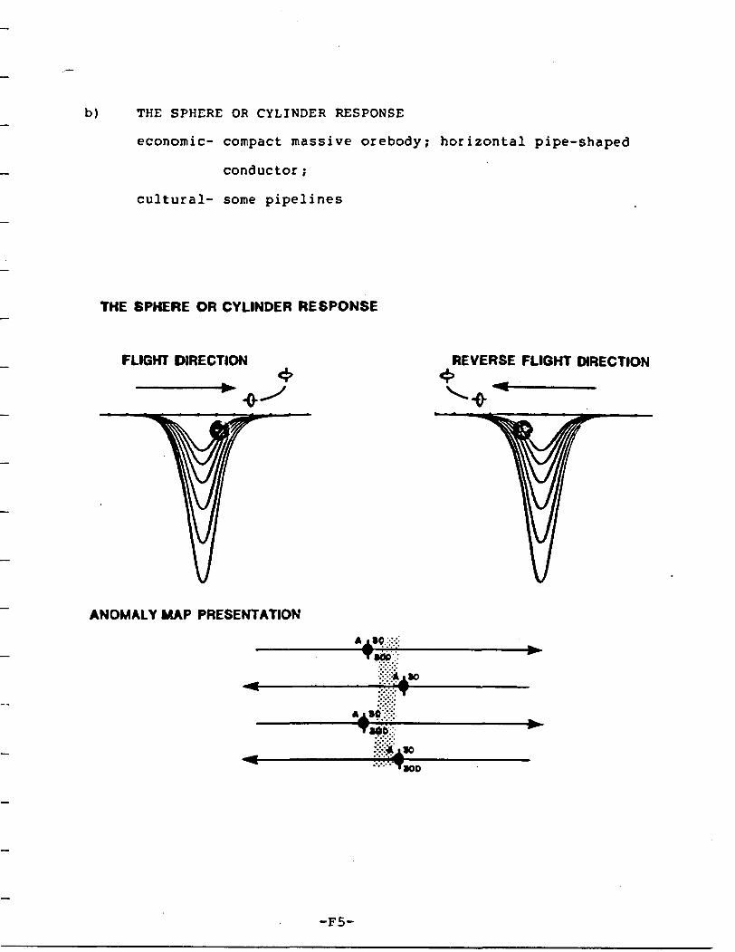
b) THE SPHERE OR CYLINDER RESPONSE

economic- compact massive orebody; horizontal pipe-shaped

conductor ;

cultural- some pipelines

THE SPHERE OR CYLINDER RESPONSE

FLIGHT DIRECTION

ANOMALY MAP PRESENTATION

V

REVERSE FLIGHT DIRECTION

'•00

-F5-

The response of a cylinder may be quite difficult to

recognize from a thin strip. A cylinder or spherical model does

not show a pronounced negative or upward peak following the main

response. Due to the effect of the time constant of the INPUT

receiver, the negative peaks which follow the theoretical response

do not appear on the INPUT records (Mallick 1972, Morrison et al

1969). As the illustrations show, the sphere-cylinder response is

perfectly symmetrical, but not centered over the body. The

plotting position of the main peak leads the actual axis location

because the most favourable mutual coupling occurs just before the

transmitter coil passes the conductive body. The amplitude of the

responses will be similar in both flight directions for a perfect

cylinder.

-F 6-

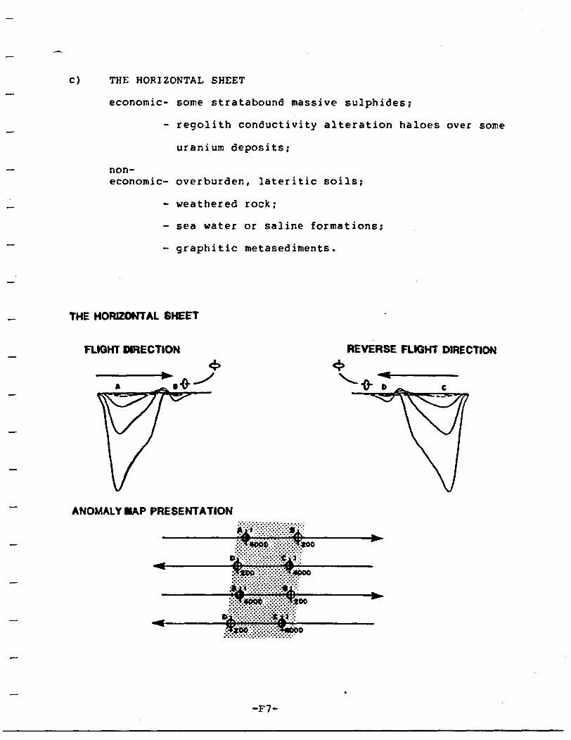
C) THE HORIZONTAL SHEET

economic- some stratabound massive sulphides;

- regolith conductivity alteration haloes over some

uranium deposits;

non- economic- overburden, lateritic soils;

- weathered rock;

- sea water or saline formations;

- graphitic metasediments.

THE HORIZONTAL SHEET

FLIGHT DIRECTION

ANOMALY MAP PRESENTATION

REVERSE FLIGHT DIRECTION

*oo

rrt4POO

too

-F7-

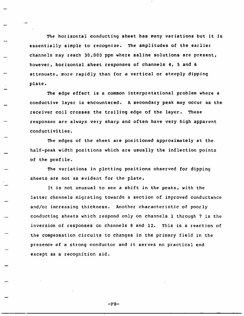
The horizontal conducting sheet has many variations but it is

essentially simple to recognize. The amplitudes of the earlier

channels r. a y reach 30,000 ppm where saline solutions are present,

however, horizontal sheet responses of channels 4, 5 and 6

attenuate, more rapidly than for a vertical or steeply dipping

plate.

The edge effect is a common interpretational problem where a

conductive layer is encountered. A secondary peak may occur as the

receiver coil crosses the trailing edge of the layer. These

responses are always very sharp and often have very high apparent

conductivities.

The edges of the sheet are positioned approximately at the

half-peak width positions which are usually the inflection points

of the profile.

The variations in plotting positions observed for dipping

sheets are not as evident for the plate.

It is not unusual to see a shift in the peaks, with the

latter channels migrating towards a section of improved conductance

and/or increasing thickness. Another characteristic of poorly

conducting sheets which respond only on channels l through 7 is the

inversion of responses on channels 8 and 12. This is a reaction of

the compensation circuits to changes in the primary field in the

presence of a strong conductor and it serves no practical end

except as a recognition aid.

-F8-

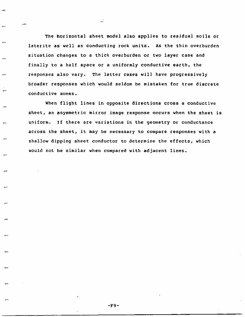
The horizontal sheet model also applies to residual soils or

laterite as well as conducting rock units. As the thin overburden

situation changes to a thick overburden or two layer case and

finally to a half space or a uniformly conductive earth, the

responses also vary. The latter cases will have progressively

broader responses which would seldom be mistaken for true discrete

conductive zones.

When flight lines in opposite directions cross a conductive

sheet, an asymmetric mirror image response occurs when the sheet is

uniform. If there are variations in the geometry or conductance

across the sheet, it may be necessary to compare responses with a

shallow dipping sheet conductor to determine the effects, which

would not be similar when compared with adjacent lines.

-F9-

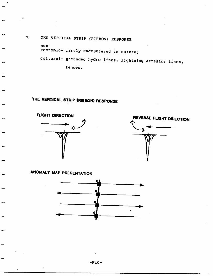
d) THE VERTICAL STRIP (RIBBON) RESPONSE

non-economic- rarely encountered in nature;

cultural- grounded hydro lines, lightning arrestor lines,

fences.

THE VERTICAL STRIP (RIBBON) RESPONSE

FLIGHT DIRECTION

ANOMALY MAP PRESENTATION

REVERSE FLIGHT DIRECTION

-F10-

Due to the fact that this type of response is most commonly

caused by fences, lightning protection lines and grounded power

lines, the customary cultural presentation is a square symbol.

This cultural response symbol may or may not have a power monitor

(50-60 cycle) response but these will normally follow pipelines,

fences, power lines, roads, railroads and other man made

structures. The amplitude and apparent conductivity of such

responses varies with the ground conductivity. In residual soils

or conductive overburden, it is often possible to see a positive

(up-dip type) peak followed by a small negative immediately before

the main conductive response. The presence and amplitudes of such

responses is normally very consistent. The cause of such responses

is interpreted to be current gathering within the surficial

sediments (West and Macnae 1982) .

-Fll-

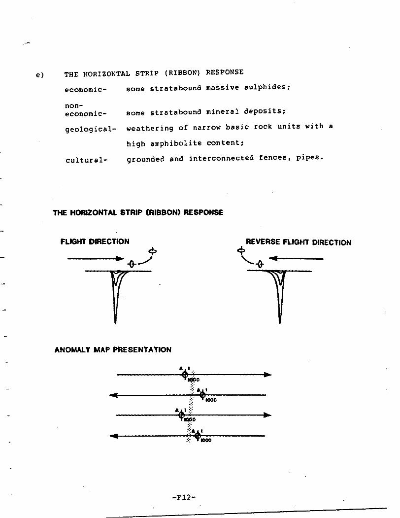
e) THE HORIZONTAL STRIP (RIBBON) RESPONSE

economic- some stratabound massive sulphides;

non- economic- some stratabound mineral deposits;

geological- weathering of narrow basic rock units with a

high amphibolite content;

cultural- grounded and interconnected fences, pipes.

THE HORIZONTAL STRIP (RIBBON) RESPONSE

FLIGHT DIRECTION REVERSE FLIGHT DIRECTION

ANOMALY MAP PRESENTATION

Ail

*woo

:-: T looo

-F12-

The plotting positions of the responses could easily be

mistaken for a vertical plate conductor, however, careful

consideration must be given to the flight direction. The

horizontal ribbon is a degeneration of the horizontal conducting

sheet. It can be easily distinguished from a sphere or cylindrical

body by its peak asymmetry, whereas the sphere model has a single

symmetric main response.

-F13-

APPENDIX G

QUANTITATIVE INTERPRETATION

The quantitative interpretation of the INPUT data is normally

accomplished by comparing the resultant responses with type curves

obtained from theoretical calculations, scale model studies and

actual field measurements. A variety of results are available in

literature for different conductor geometries and system

configurations (see Ghosh 1971, Palacky 1974, Becker et al. r 1972,

Lodha 1977, Ramani 1980). They have also examined the effects of

varying such parameters as conductance, conductor depth, dip and

depth extent. Their approach has been successfully applied in

interpretation of past field surveys.

The nomograms which are currently available for the INPUT

system are the Vertical Half-Plane, Homogeneous Half-Space, Thin

Overburden and 135 Dipping Half-Plane nomograms. The first is

particularly useful for the interpretation of vertical dyke-like

conductors frequently found in the Precambrian Shield type

environments. In the case of a thick, homogeneous, flat-lying

(less than 30 dip) source, the Homogeneous Half-Space nomogram

should be applied. While in a thin overburden or tropically

weathered rock environment, the Thin Overburden nomogram may be

referenced to determine the depth and conductance of the overburden

(Palacky and Kadekaru, 1979).

As an example, INPUT anomalies due to vertical dyke-like

conductors, are asymmetric and independent of the flight direction.

-Gl-

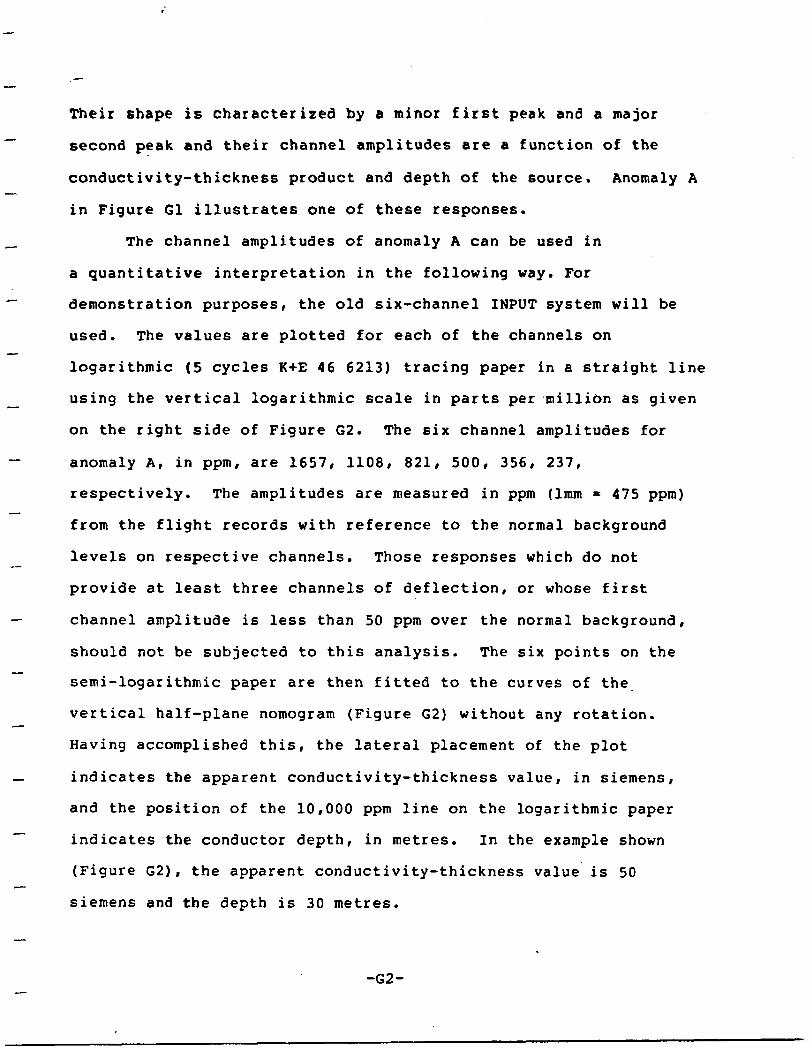
Their shape is characterized by a minor first peak and a major

second peak and their channel amplitudes are a function of the

conductivity-thickness product and depth of the source. Anomaly A

in Figure Gl illustrates one of these responses.

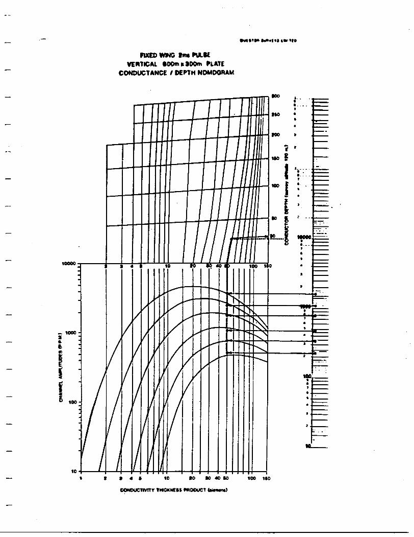
The channel amplitudes of anomaly A can be used in

a quantitative interpretation in the following way. For

demonstration purposes, the old six-channel INPUT system will be

used. The values are plotted for each of the channels on

logarithmic ( 5 cycles K+E 46 6213) tracing paper in a straight line

using the vertical logarithmic scale in parts per million as given

on the right side of Figure G2. The six channel amplitudes for

anomaly A, in ppm, are 1657, 1108, 821, 500, 356, 237,

respectively. The amplitudes are measured in ppm (1mm - 475 ppm)

from the flight records with reference to the normal background

levels on respective channels. Those responses which do not

provide at least three channels of deflection, or whose first

channel amplitude is less than 50 ppm over the normal background,

should not be subjected to this analysis. The six points on the

semi-logarithmic paper are then fitted to the curves of the

vertical half-plane nomogram (Figure G2) without any rotation.

Having accomplished this, the lateral placement of the plot

indicates the apparent conductivity-thickness value, in Siemens,

and the position of the 10,000 ppm line on the logarithmic paper

indicates the conductor depth, in metres. In the example shown

(Figure G2), the apparent conductivity-thickness value is 50

Siemens and the depth is 30 metres.

-G2-

FIXED WMG fm PULSEVERTICAL tDOmk)DOm HATE

CONDUCTANCE l DEPTH NDMDORAM

**r|t| l*

10X * 4 S 10 tO *0 40 *0

coNDucnvrrv TMCKNESS PRODUCT towmm)

100 1*0

QUESTOR INPUTTHIN PLATE DIP ESTIMATION

and AMPLITUDE NORMALIZATION GRAPH

•e mx co

3D 40 60 fop) 70 Ve 90100110120130140150

DIP - DEGREES

\1*0

Figvire G3

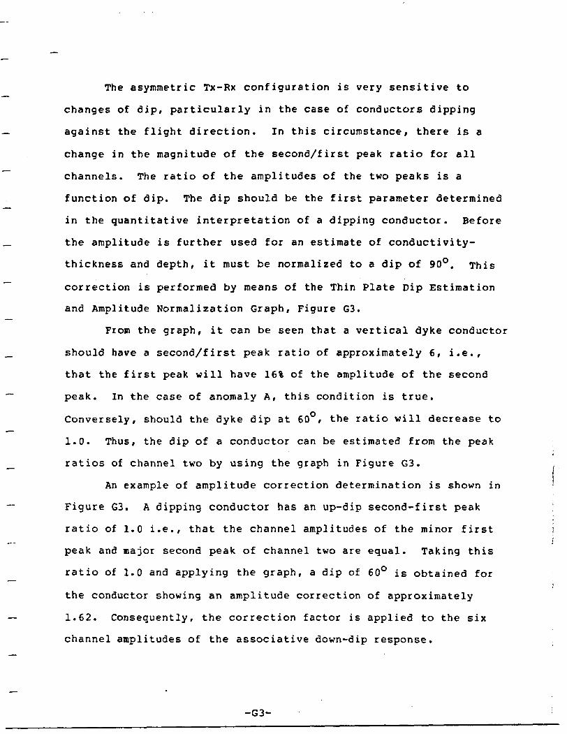
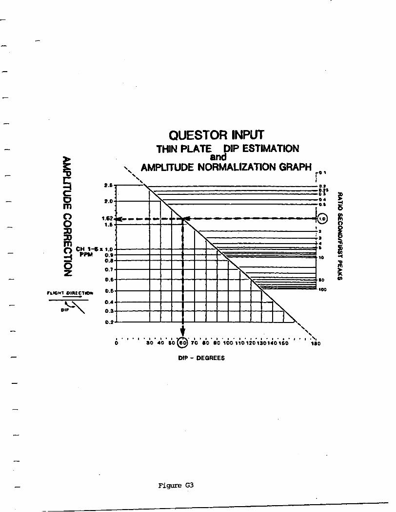
The asymmetric Tx-Rx configuration is very sensitive to

changes of dip, particularly in the case of conductors dipping

against the flight direction. In this circumstance, there is a

change in the magnitude of the second/first peak ratio for all

channels. The ratio of the amplitudes of the two peaks is a

function of dip. The dip should be the first parameter determined

in the quantitative interpretation of a dipping conductor. Before

the amplitude is further used for an estimate of conductivity-

thickness and depth, it must be normalized to a dip of 90O . This

correction is performed by means of the Thin Plate Dip Estimation

and Amplitude Normalization Graph, Figure G3.

From the graph, it can be seen that a vertical dyke conductor

should have a second/first peak ratio of approximately 6, i.e.,

that the first peak will have 16% of the amplitude of the second

peak. In the case of anomaly A, this condition is true.

Conversely, should the dyke dip at 60O , the ratio will decrease to

1.0. Thus, the dip of a conductor can be estimated from the peak

ratios of channel two by using the graph in Figure G3.

An example of amplitude correction determination is shown in

Figure G3. A dipping conductor has an up-dip second-first peak

ratio of 1.0 i.e., that the channel amplitudes of the minor first

peak and major second peak of channel two are equal. Taking this

ratio of 1.0 and applying the graph, a dip of 60O is obtained for

the conductor showing an amplitude correction of approximately

1.62. Consequently, the correction factor is applied to the six

channel amplitudes of the associative down-dip response.

-G3-

This response is then fitted to the vertical half-plane nomogram

for the determination of its apparent conductivity-thickness value

and depth. It should be mentioned that without the dip correction,

the depth would be overestimated.

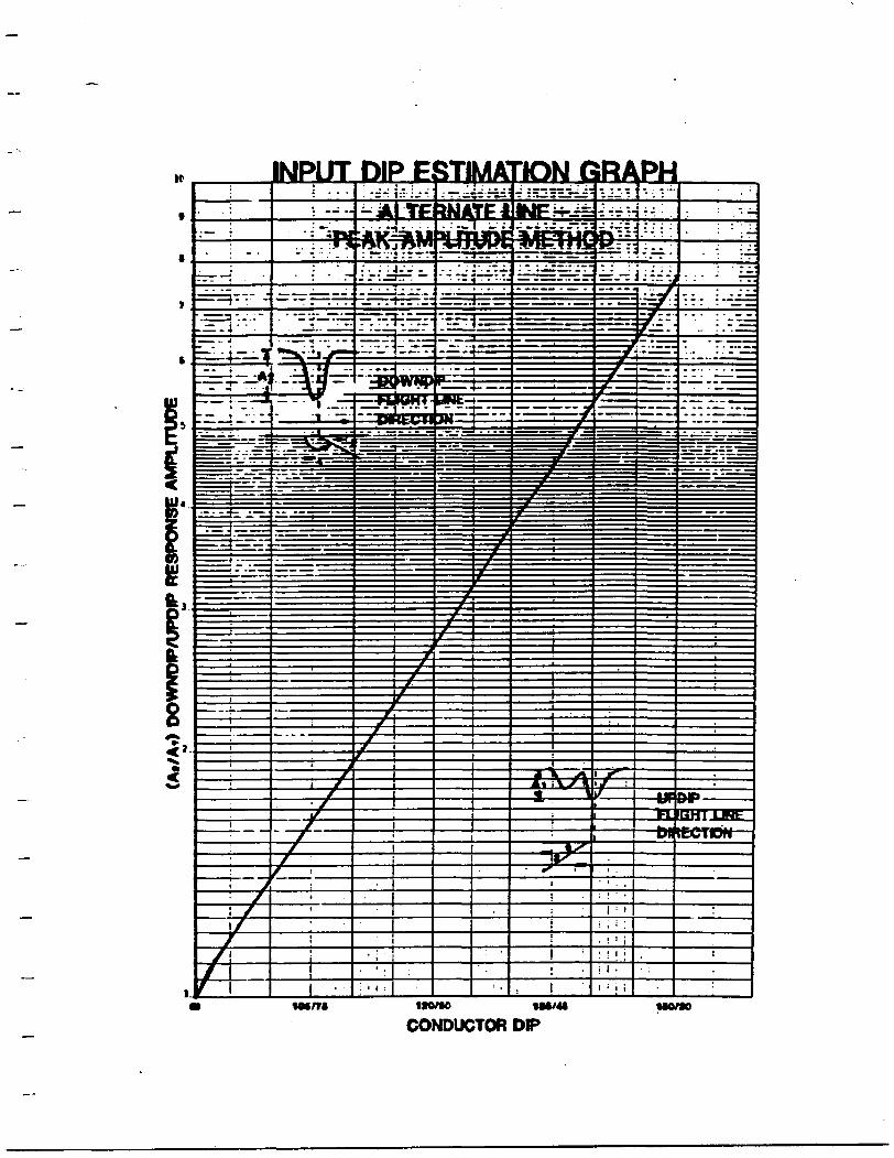
An alternate method for estimating the dips of longer,

tabular conductors, utilizes the peak amplitudes on adjacent lines,

see Figure G4. It is especially useful in multiple conductive

zones where the up-dip responses may be obscured or yield false

values due to the superposition of other nearby anomalies.

Note that the depth determination is made with the assumption

that the aircraft is at 120 metres above the ground surface at the

time of measurement. If the aircraft is above or below the

altitude of 120 metres, the depth determination can be corrected by

respectively, subtracting or adding the difference in altitude,

within lir.its. In the case of Anomaly B, Figure Gl, the anomaly

was intercepted at an aircraft altitude of 131 metres. Therefore,

a correction factor of 9 metres must be subtracted from the depth

of the conductor, placing it at 21 metres below the ground surface.

The homogeneous half-space, thin overburden and the dipping

half-plane 135O nomograms are used in the same fashion as that

described above for the vertical half-plane.

-G4-

To estimate the apparent strike length of a conductor, the

ends of the conductive trend must be determined. Modelling has

shown that the conductor ends are delineated by INPUT responses

having channel amplitudes not less than 4(H of those typical for

the conductor. Responses with less than that of 401 are

attributive to lateral coupling effects and are not considered as

intercepts of the conductor. This is especially true for

conductors of higher conductivity. Subsequently/ the strike length

of a conductor is equal to the distance between those responses

representing the ends of the conductor.

-G5-

INPUT DIP E

1IW*0

CONDUCTOR

APPENDIX H

MAGNETOMETER; COMPENSATION, SURVEY AND PROCESSING

Aircraft Magnetic Compensation

In order for a high sensitivity magnetometer system to

function without interference from the aircraft, it must be

magnetically compensated. The sources of magnetic interference,

produced by the aircraft are: a) eddy currents; b) aircraft

electrical system; c) induced magnetism; and d) permanent

magnetism. These sources of magnetic noise have distinguishable

characteristics on the analogue records and a ground and airborne

test will indicate the capabilities of the magnetometer

installation. By following established procedures most of the

noise sources are eliminated.

a) Eddy currents are caused by movements of the larger

conducting surfaces of the aircraft in the earth's magnetic

field, whereby electric currents are generated, causing

magnetic fields. By placing the-sensor at the greatest

practical distance from these surfaces and by not flying in

turbulent wind conditions, eddy current noise can be

minimized.

b) Aircraft electrical systems with varying loads can lead to

serious noise problems if consistent operations procedures

and circuit layout are not properly designed. The switching

-HI-

of the aircraft's 28 volt DC to almost any component during

survey will create a variation in the static field existing

under normal operating conditions. The three component

compensator in the aircraft will see electrical system noise

as DC level shifts from a heading invariant datum.

c) Induced magnetic fields are produced by ferromagnetic parts

(mainly engines) in the earth's magnetic field. For a major

change in magnetic latitude, it is necessary to check for

variation of the aircraft's induced magnetic field. This is

also dependant on the aircraft's heading and altitude.

Compensation is accomplished by critical positioning of

permalloy strips near the sensor. These produce fields

opposite to the induced magnetic field of the aircraft,

effectively cancelling it.

d) Permanent magnetism is produced by ferromagnetic parts within

the aircraft. Compensation is accomplished with three

orthogonal coils, through each of which an electrical current

is passed, to create a resultant stable field opposite in

polarity to the permanent field.

The compensation process has as its main objective the

reduction of heading errors. These may be checked by flying the

aircraft at survey altitude over a well defined non-anomalous

landmark in the four cardinal headings. In addition, the effects

of aircraft flight characteristics on the magnetometer install

ation are simulated by performing roll, pitch and yaw maneuvers.

-H2-

The aircraft has been originally compensated in Toronto,

Ontario, where the induced field has been cancelled. . In the survey

area, a check is made to ensure that the permanent field does not

induce heading dependant, magnetic field errors.

MAGNETOMETER SURVEY AND DATA ACQUISITION

The magnetometer survey is an integral part of INPUT

operations, with no special procedures being required; with the

exception of a ground magnetic recording station to monitor daily

diurnal variations. The diurnal survey specifications relate to

the control line spacing to minimize the-possibilities of erroneous

contours in area of low magnetic gradient.

The maximum diurnal gradient permitted is 20 nanoteslas

change within 5 minutes. The maximum control line spacing allowed

is 8 kilometres. Where possible, control lines are routed through

areas of low magnetic gradient over easily identified topographic

points. As the time for the survey aircraft to span two control

lines is approximately 2 minutes, a maximum diurnal anomaly of 4 nT

(nanoTeslas) may exist after the data has been levelled.

The daily variation of the earth's magnetic field is

monitored and recorded with a Geometrics G-826 Base Station

Magnetometer and a GULTON or Hewlett Packard Strip Chart Recorder.

The recorder has a 10 cm. chart width with a 100 nT full scale

deflection, providing scaling of l nT/MM. An event marker provides

time reference marks every minute. The chart speed is set to

20 cm/hour, with magnetometer readings taken every 4 or 10 seconds.

-H3-

These readings may be digitally recorded using a portable data

acquisition system synchronized with the aircraft data system, if

required.

The magnetometer readings in the aircraft are recorded every

second onto industry standard, 9-track tapes using the IBM NRZI

Format.

-H4-

APPENDIX I

Bibliography

Barringer, A.R., 1962, The INPUT Airborne Electrical Pulse

Prospecting System: Min. Cong. J., volume 48,

page 49-52;

Barringer Research Limited, 1962, Method and Apparatus for the

Detection of Ore Bodies: United States Patent

Office: 3.020,471;

Barringer Research Limited, The Quantitative Interpretation of

Airborne INPUT Electromagnetic Data: Barringer

Research Technical Note;

Becker, A., 1969, Simulation of Time-Domain, Airborne

Electromagnetic System Response: Geophysics,

volume 34, page 739-752;

Becker, A., Gavreau, D., and Collett, L.S., 1972, Scale Model Study

of Time-Domain Electromagnetic Response of Tabular

Conductors: CIM Bull., volume 65, number 725,

page 90-95;

Dyck, A.V., Becker A., and Collett, L.S., 1974, Surficial

Conductivity Mapping with the Airborne IKPUT

System: CIM Bull., volume 67, number 744, page

104-109;

Ghosh, M.K., and West, G.F., 1971, EM Analog Model Studies: Norman

Paterson and Associates, Toronto;

-II-

Lazenby, P.G., 1972, Examples of Field Data Obtained with the INPUT

Airborne Electromagnetic System: Questor Surveys

Limited;

Lazenby, P.G., 1972, New Developments in the INPUT* R ' Airborne EM

System: CIM Bull., volume 66, number 732, page

96-104;

Lodha, G. S., West, G. F., 1976, Practical Airborne EM (AEM)

Interpretation Using a Sphere Model: Geophysics,

volume 41, page 1157-1169;

Mallick, K., 1972, Conducting Sphere in Electromagnetic INPUT

Field: Geophysical Prospecting, volume 20, page

293-303;

Macnae, James C., 1979, Kimberlites and Exploration Geophysics:

Geophysics, volume 44, number 8, page 1395-1416;

Mishra, D.C., Murthy, K.S.R., and Narain, H., 1978, Interpretation

of Time-Domain Airborne Electromagnetic (INPUT)

.Anomalies: Geoexplor., volume 16, page 203-222;

Morrison, H.F., Phillips, R.J., and O'Brien, D.P. 1969,

Quantitative Interpretation of Transient

Electromagnetic Fields Over a Layered Half-Space:

Geophys. Prosp. volume 17, page 82-101;

Nelson, P.H., and Morris, D.B., 1969, Theoretical Response of a

Time-Domain Airborne Electromagnetic System:

Geophysics, volume 34, page 729-738;

Nelson, P.H., 1973, Model Results and Field Checks for a

Time-Domain Airborne EM System: Geophysics,

volume 38, page 845-853;

-12-

Palacky, G.J., and West, G.F., 1974, Computer Processing of

Airborne Electromagnetic Data: Geophysical

Prospecting 22, page 490-509;

Palacky, G.J., and West, G.F., 1973, Quantitative Interpretation of

INPUT AEM Measurements: Geophysics, volume 38,

page 1145-1158;

Palacky, G.J., 1974, The Atlas of INPUT Profiles: B.R.L. Toronto,

page 37;

Palacky, G.J., 1975, Interpretation of INPUT AEM Measurements in

Areas of Conductive Overburden: Geophysics,

volume 40, page 490-502;

Palacky, G.J., 1976, Use of Decay Patterns for the Classification

of Anomalies in Time-Domain AEM Measurements:

Geophysics, volume 41, page 1031-1041;

Palacky, G.J., 1977, Selection of a Suitable Model for Quantitative

Interpretation of Towed-Bird AEM Measurements:

Geophysics, volume 43, number 3, page 576-587;

Palacky, G.J., and Kadekaru, K., 1979, Effect of Tropical

Weathering on Electrical and Electromagnetic

Measurements: Geophysics, volume 44, page 21-38;

Palacky, G.J., and Sena, F.O., 1979, Conductor Identification in

Tropical Terrains - Case Histories from the

Itapicuru Greenstone Belt, Bahia, Brazil:

Geophysics, volume 44, page 1931-1962;

-13-

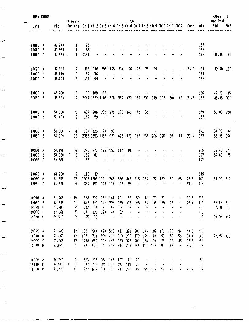
JOB: 88032

Line

10010 A10010 610010 C

10020 A10020 B10020 C

10030 A10030 B

10040 A10040 B

10050 A10050 B

10060 A10060 B10060 C

10070 A10070 B10070 C

10080 A10080 B10080 C100?0 P10090 E

inner! A10090 B10000 C10090 0

10100 A1-0100 B30300 C

Fid

40.2*040.96041.480

42.86043.14043.700

47.78048.890

50.80051.490

54.80055.990

58.39059.06059.760

63.2606*. 70065.340

65.66066.84067.60065.1606S.510

71.01072.45077.56073.090

74.7^0n rxn75 . ? ?0

Anoialy Typ Chs

111

922

312

82

P 412

6P 2

1

212

6

L1 1C11

4c

2

1?1?1?11

71! 7

1 1

Chl

750600

1151

40847

132

992041

437162

1572388

371152oc05

1182007

389

36861814214155

103]1071123890?

323w8P ?

Ch 2 Ch 3

316 29636 -64 -

100 881522 1165

206 28859 -

125 791653 1353

272 19581 -

32 -1508 1221

192 193

299 23744] 376

51 9!126 129

15 -

811 690761 56.Q85? 700670 5?7

20? 168w 2^629 5]0

Ch 4

175-~

—

808

171"

93930

150-

^

76'118

1642?3

6?it-

56?t"t-. 1369

i/e"/'i "

t j:

Ch5

134-"

.557

172"

.625

117-

^

55693

101165

-52-

411313373245

10712?243

EI Ch 6

96-~

.452

146"

.471

91-

^

44895

83113

---

391235326203

711192??

1 Ch 7 Ch 8 Ch 9 ChlO Chll Chl2 Cond

96 76 39 - - - 35.0." " ~ ~ " ~

.282 230 179 113 96 49 24.5

73 58 - - - -.

.315 237 206 120 98 44 21.6

.

.

m. V — — * w

315 236 177 132 89 65 28.5- - - - - - 38.4

52 74 70 30 - - 30.565 60 45 50 2' - 24.6...

28] 245 187 ]6 C 125 94 44.217? 129 94 95 76 56 34.4201 148 121 8e 76 45 35.91*1 107 108 90 3? - 26.5

27 - - - . -70 - - - - -Of O R ]fl' C7 ^7 . 71 q

Alt

137top130137

164144129

126138

179153

151153

21616710lo/

ii91611"

:?8i??i? c.•7r

1 : ~'

"?-i160•'C

:' f

i ri* ' *'^^

PAGE:Mag Peak Fid

41.45

42.90

47.7548.85

50.80

54.7555.95

58.4059.00

64.70

66.8567.70

68.60

7?. 45

1

Val

fivi

150

35300

228

44296

3?:75

5 7 ?

5":*,-

2r.;

4;:

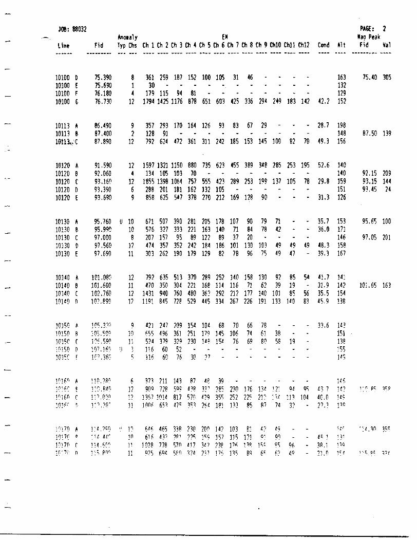
J 06: 88032

Line

10100 010100 E10100 F10100 6

10113 A10113 B10113,, C

10120 A10120 B10120 C10120 D10120 E

10130 A10130 610130 C10130 010130 E

10140 A10140 B10140 c10140 P

10150 A10150 B10 ici0 C•0150 D10150 F

1016 n APlfiC; f.

in: fin r101 6-r n

'::Vi7fl fi.10170 ai? 'i 70 C^•''.1'} n

Fid

75.39075.69076.18076.730

86.49087.40087.890

91.59092.06093.16093.39093.690

95.76095.99097.00097.56097.690

101.080101.600102.76010?. 890

105.3?'1!0-'.50nine qonK'7.160107 ' 36 -

110.7BPr. 0.840r^. o o^i:-'.?o-

1^.700Mi H ?114 fi™1:-. P n "

Anoialy Typ Chs

814

12

92

12

124

1269

U 1010

81211

12111212

Q1011

U 35

fi121211

1; 10inrn

Chl

36130

1791794

357128792

1597134

1855288858

671576207474303

792470

14311191

421655574116116,

37390 Q

136?100f

Wfi616

10780 ?5

Ch 2 Ch 3

259 187

115 941425 1176

293 17091 -

624 472

1321 1150105 103

1398 1064201 181625 547

507 390327 333157 95357 352262 190

635 513350 304940 760845 728

247 209496 361379 320

60 5260 76

711 143728 599

101' 81765? 47 C

465 33843? ?? 1778 5?n694 5PO

Ch 4

152

81878

164-

361

88070

757162378

281221

89242179

370221480529

154251230

30

8743?57035?

230m417

EI ChSCh 6

100 105

-651 603

126 93-

311 242

735 623-

555 423132 105270 212

205 178163 140122 89184 186129 82

289 252168 11436? 292445 334

104 68179 14514? 154

.7?

4? 393? ? 285no 35*;26' 181

?0 r 14?1" 157347 7^P757 175

H Ch 7 Ch 8

31 46

-425 336

83 67-

185 153

455 389-

289 253-

169 128

107 9071 8437 20

101 13078 96

140 158116 71217 177267 226

70 66106 74

76 69

"

.230 176252 225133 85

103 8!115 17117fi 1?P135 83

Ch9

-294

29-

145

348-

199-

90

7978

-10375

13062

14C191

786180

-

.13'71'

87

4?01

KG6 C

ChlO

-249

-

-100

285-

137-~

7142-

4949

9239

101133

^

3858

~

.1 ? 1\\l

74

'990pc;6^

Chll

-183

^

-82

253-

105-~

-

--

4947

851985

140

.-

19

-

04113

3?

.-

96P

Chl2

-147

—

-70

195-

78-™

^

--

49~

54-

5683

.-

.

-

-

.OR

104-

.-^.

Cond

42.2

28.7

49.3

52.6

29.8

31.3

35.736.0

48.339.3

41.731.935.545.9

33.6

'?.740.0?7.?

'P 138.121.0

Alt

163132129152

198148156

140140159151126

153171146158167

14]142154138

143151138

1'9

K61'?149H'

•If'nino15*

PAGE: 2Mao Peak Fid Val

75.40 305

87.50 139

92.15 20993.15 14493.45 24

95.65 100

97.05 201

101.65 163

r. r p c w

M.',30 355

;.'d.?E. v t

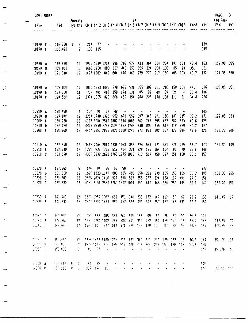
M: 8803

Line

10170 E10170 F

10180 A10180 810180 C

10190 A10190 B10190 C

10200 A10200 B10200 C10200 D10200 E

10210 A10210 B10210 C

10220 A10220 B1"220 C10220 D

1 : 230 Ai"3o B

i::-'o A":"'*o B!"'4? f"

•"P f.'"'^0 P- i - n r

2 t

Fid 1

116.380116.490

119.890121.060121.310

123.060123.360224.560

128.480129.040130.220130.260130.360

132.310132.540133.690

137.660135.3001??. 500135.680

li; .449K: .630

I'V^O1^,560}i- . 5^1

ir.^n': : ' '70

ir- p -r,

moialy yp Chs

U 22

121212

121112

412121212

121212

5121212

1212

123?r/

r,17

•j

Ch 1 Ch 2

214 77138 115

1955 15391668 1160142 7 1002

1856 139370? 481

1374 1005

100 962254 1740'12? 30844446 33504 T. 7 3350

34'5 24641251 935'306 3239

1*6 941695 1320260- 1824'15! 3354

if c' Y'™23*7 ipr,7

11- 5 ?71 G * ' 1 *Qi1?:~ C5~

1??:' ;*15Y~*~'' \\^~i

f- r

Ch 3 Ch 4

-

1264 896893 607846 604

1093 778418 259810 606

67 491378 9522519 18022793 20242831 2026

2014 1386766 519

2628 1768

65 551140 8031416 9272550 1760

100? 6121473 99?

'85 3581102 7487?? 514

11*0 79597? 6?5

.

FICh 5 Ch 6

-

716 578448 355476 366

623 531194 131430 35'

.6?3 552

1376 10821553 12481600 1291

1058 855404 324

1275 1018

50 -605 493688 512

1302 1019

'51 344752 59?

26? 199583 471371 m

633 45?^6 408

-

1 Ch 7 Ch 8

-

433 364259 224279 270

385 30785 92

268 226

.397 343862 745930 805973 821

624 541229 176712 569

.358 291358 287751 610

233 17240? 347

136 99310 2521*? 12P

3*0 31?309 2'5

.

Ch 9 ChlO

-

304 23'208 130217 130

261 20549 39

170 131

.271 190595 462655 51?682 55?

421 331164 104450 327

.239 16522* 180466 336

14P 11225 1 18?

82 781?? 35^120 S 1

?i? 179213 150

-

Chll

"

19185

103

15926

111

.147382419422

27696

251

.15311?259

8?115

8712172

153130

.

Chl2

-

16394

103

132-

91

.115323359385

22570

188

.10610f.195

67139

y.113

C.C

],C

li?.

Cond

43.435.140.7

44.126.434.4

32.240.640.243.0

38.736.830.3

36.22Q.332.0

28.932.9

30.835.7?d.9

36.6?7,8

AH

139145

163131132

136146176

145171129127126

1*3149157

1371851511*7

138151

1711*?1*6

1'i1501*3

PAGE: 3 Nag Peak Fid Val

119.90 285

121.35 350

123.05 301

129.05 333

130.35 206

132.30 149

138.30 265

139.70 150

141.45 17

148.55 ??1*S.85 53

151.00 "l 7

^^•> 70 in

.610

.160c;

86145

15MO l -:'-

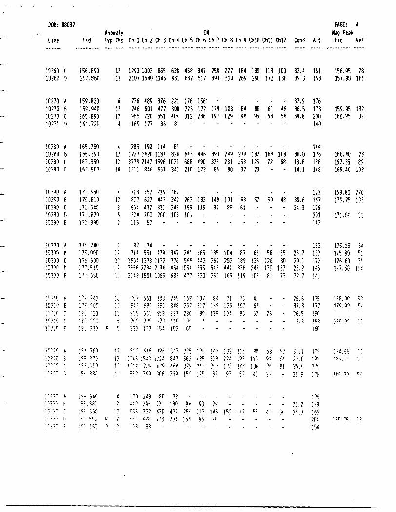
m-.Line

1026010260

102701027010?7030?70

10280102801028010280

1D?9010200102901029010290

303001C'30010300:C??0i r n fi

* r\ ^ i f|3D: 0- ". ^ n

in? rI 1.'?:'"1

•,r.r.r,

P-.'Op??r. . .* .' ! '

r:;"'33'':-:;-- . rf i

8803

CD

ABCD

ABCP

ABCPE

ABCP'F

,BfnF

t.

pf•'

iP.r

F

2

Fid

156.890157.860

159.820155.94016:. 89016:. 720

165.750165.390ir. 35016". 500

PC. 65017:. 810171.640P'. 820PI, 390

175.240175.000Pt. 600l 7 '. 510P\ 650

P .7*?P .900!5 '20:? :?0:?:.-3?

,C, , fip•c: 370;c.- -nri•c- 3fin

! ; .5*01? .SfiOP 56?\ r" ^0Y- . } 6 0

Anotaly Typ Chs

1212

61212

4

4121210

412

952

2PPi?i?

3?1?11

6o c

12PP1 1

i7

17

P 7P 2

Ch 1 Ch 2 Ch 3 Ch 4 Ch 5

1293 1002 865 638 4582107 1580 1186 831 632

776 489 376 221 178746 601 477 300 225965 720 551 404 312169 177 86 81 -

285 190 114 81 -1727 1420 1184 828 6433278 2147 1596 1021 6881311 846 561 341 210

713 352 219 167 -8?7 627 447 342 263654 437 333 248 169?2* 200 200 108 101115 57 - - -

87 34 - - -714 551 429 347 2*1

3954 1378 1132 776 56P?*:* 2784 2194 1*54 105*2:*8 3503 1065 683 4?7

7 f? 563 383 245 168cj7 557 591 3*8 ?c;-V.5 663 553 33? 236ve ?2P 173 lin 3f23? 1.73 15* 10? 6 C

cin fif, apf 347 7^~'t', ] s^o j??/; p*7 5f?1-1 C; 7PO pa ( f,t ?9C-'7 ' QQ ^06 ?3 Q 150

PO 143 80 7P::i ?9S 221 180 9'0 55 73? 630 4?? ?? ;c :' : ^?P ?78 20.1 354

O fi 3P

EICh 6

347517

156-172236

~

.496490173

.183119

--

.165443735320

137237Igo

/l-

37*4 '5?0PC

.

93

96-

Ch 7

258394

.129197

*

.393325

85

.34097--

.135267543250

84369139

--

1/7?r'81'~!

8'

.79i^7r

-

Ch 8

227310

.108129

"

^

299231

80

.10388--

.104252ill165

71126IP*

--

in-2'-'3^e?7

.-

35?--

Ch 9

184269

.8494

"

.270158

3?

.9?61--

.87

189338139

75107

85--

r. fior3"

C 1

.'

117--

ChlO

130190

.8895

~

.187125

23

.57---

.63

135243105

41675?--

9P33330^

40

.-

55--

Chll

113172

.6168

~

.16372

"

.50

---

.58

126PO8]

.-

25--

599"Kr.-

.-*'---

Chl2

100136

.4654

~

.10868

"

^

48---

.3580

13773

.----

CI

5-!

83-

.-

ir--

Cond

32.439.3

37.936.534.8

38.018.814.1

30.624.3

26.729.126.222.7

25.637.326.52.3

33.123.035. n25.o

25.2?5.3

AH

151153

176173200140

144176138148

173167196201147

13213717?1451*1

175177180lop160

HQ3 C'117P3^6

37517936520435*

PAGE: Mag Peak Fid

156.95157.90

159.95160.95

166.40167.35168.40

169.80170.75

173.80

175.15175.90376.60377,50

178,00375. Of

18C.9"1

M.F1?-.^

IP', "'f1

18 f 75

Vi 1

28166

13?3?

2889

1P3

27030?

2:

; f

513^

1C*

C. CCi

- '

. -

k *

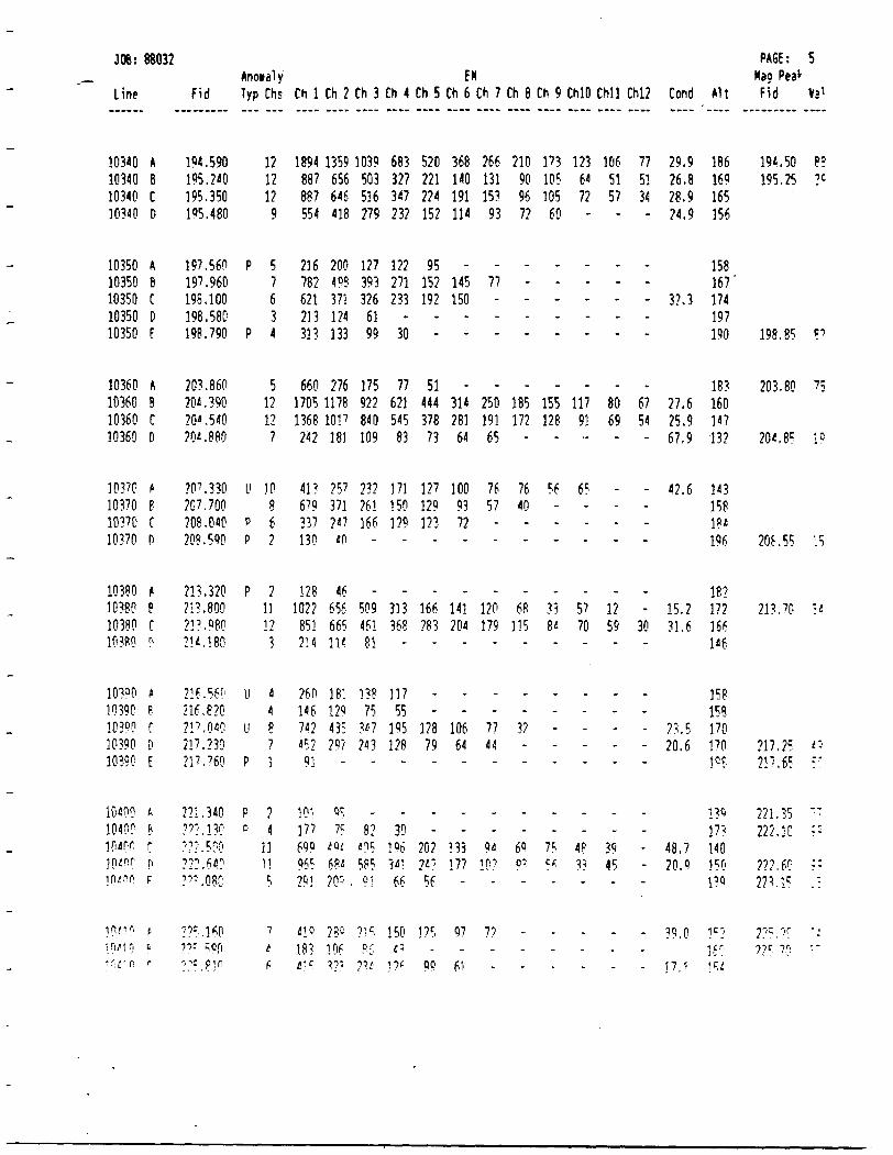
. : iji bit

:- ^:: O9'i22

:: Gl'222:. 58-122

.: 59712•:? 52 712

?- Oi'8I2

Si SS'302

ci 58 '702

Si OS'802

ts S8'86I

se 52 '561

i'* PH

S" IflUJ * 33 TO

cii O'bt

btl051 b'02OH i'8frtilbtl

SolOil 9'02Oil S'82851351

9H991 9'lt2il 2'SI231

9617fil851871 9'27

281 6'i9iH 6'52091 972831

061i6lW 878

.i9I851

9SI 6'72591 6'82691 8'92981 6'62

J W PU03

.

-57 tt 95 to68 d7 Si 69

.

- ' - - -

-- - - - 28-

. - . .

-

08 6S Oi 78 Sil- 21 iS 88 89— — — — —

--- - - - 07

- 59 95 9i

- - -,

75 69 16 821 2ili9 08 ill SSI 581" ~ ** ~ ~

~-.-~ * ~ ~ ~

- - - 09 2i78 iS 2i SOI 96IS IS 79 SOI 06ii 901 821 Eil 012

2143 1143 0143 6 43 8 43

ii

.

cUt?6-—

77ii-~

.

bil021~

.

-

iS9i

59tot052~

.--ii—

86851181992

i 43t

19 ob

ib bil

- 95iii i?2881 202-"" ""

79 6i901 821-" ~

-

702 882IH 991

— ~

,

2i 82186 621001 i2l

79 8i182 8i8HE 777- IS

.-OSI 261SH 251- 56

HI 251161 722OH 122898 025

9 43 S 43 13

t? OSI

99

96108"*

821S6I55ill

^

398818~

.

621OSIlil

88S7S129ii

OE-882lil221

282i78i2E889

F 43

9a bti

Lobdb5Cft8"

872i7tSi881

13I9f605~

.

991i92282

601078226Sil

6619928868i2l

6i29ISEOS6801

E 43

:U J, 7901 881582 OL7

' ;02 tbi?89 556Jo? o69bi Lilbb iOl

16.uc 63?^C b 7 B y

621 971181 092

HI 712599 158959 220197 821

O? 081i72 i88liE 6i9tS2 tl*

181 2?2ilfll 8981Sill SOil9i2 099

881 818721 812liE 129867 28i002 912

81* 7SS979 i88959 i886S8I 7681

2 43 I 43

9 7 i

5ttII72

li877

t21li2

298Oi

i2121S

F89iS

6212121

dd

d

nn

d

dd

n

d

d

S43 ^i X^eiouy

Oy l 'iii

080 '.-.i :uWa2uOS c 1 1ut t 'it i078' lit

09fiu082712G70'tlt028 '9lt095 '9 tt

08l'7itG86'(-t2008 't liO28'ti2

065 '802070-80200i'i02088702

088'70207 S "702068 '702098 '802

06i'86I08S'86loorsei096 761G9S761

OSF'Sol058 '561OF2'S6l065 '76 l

PU

J J.J'j:

i Ou'Oli iji?0i

J 'JU7Ut

0 JUJufJ J07GI^ OOfOlV UU70I

3 06801(i 06801J uo80iS 068011 GctOI

0 08801J 088018 08801i 08801

0 OitOI3 OitOI9 Oi80li OitOI

0 098013 098018 09801V 09801

d OS80I0 058013 OSEOI9 OSEOIV OS801

0 078013 OKQl9 07801i OFEOl

JUL]

2E088 :90f

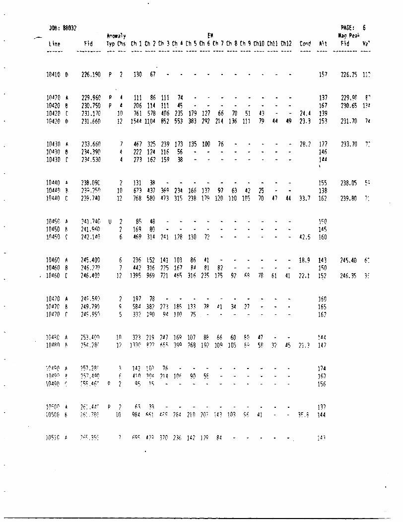
t?ifi o2l til 9t2 Oii ci?-Jit 'ir:(HiGC

•E SE'972

:-9 O? '5*2

'.L 08'6E2

•S SO'8E2

.'i Oi'EE2

it Oi'lE2

lil S9'OE2J 06 '622

;il S2'922

M PH

77t S'itiEI

951i9t7il

W i' li7H

291S91091

251 I'llOilEH 6'8l

091 S'27SHObi

291 i'EE8EISSi

7H9Hiil 2'82

ESI E'E26CI 7'72i9liEI

iSl

UV P"03

[7 35 tO i t7t 'M

- -

X - - -

S7 Li aS o3 SOI 601 261- - i7 -j s 09 99 38

- - - - .

i2 7E 17 8i"" "* "* ~ * — ~

rt 19 8i 89 26 Sil St2- - - - - 28 18- - - - - - rt

- - - - - - 2i.~ "* *" ~ *~ ~ "*

77 i7 Oi SOI Oil 021 oil- - 52 27 E9 i6 itl" ~ ~ ~ ~ ~ ~

.-- - - - - 9i 001

67 77 6i III 9EI H2 262- - t? IS Oi 99 Lil -" ~ ~ ** " "

-

2143 1143 0143 6 43 8 43 L 43 9 43

012

^

06~

892iOI

SiEEl™

9 IE7898

OEl-~

8E2991~

.

-SCI

E8E6il-"

-

543

?82

.

901"

o6E691

GO lS8I~

Wi9lEOl

821-~

SIEfE2~

8E9SEi I

ESSSE2577i

-

7 43

Oi7

^

1119i

bS9i 72

76ILI~

IIL522IH

l W-~

EiPo9E™

6519116E2

258907IIIIII

-

E 43

tt

itJutiOI

Lin612

Ool28E8i

69691E251

HE0887

085iE78E

291721S2E

70118iSHI98

L9

243

ty

StUl7it l

OEElE2E

2tt?8Si6l

Sbtl2779E2

697691b8

89iEi9IEI

Ei2222i97

7751I9i902III

OEl

I 43

01 2 d

2 d9t

21Ut

S62

21i9

922 n

21012

77i

21017 d7 d

2 d

S43 dA|

-7'

'M

JO f'.82'

u82-.07'

Ubo'Obi'G6S'

UU7'Gi2'007'

o?rOi*6' on-

07i'ub2'060'

OES'06E'099-

099'Oil1OSi'096 '

061'

P

^'3b;

i.52 •iSi

7S2 •ESZ

5726?2572

972972S72

272rt2172

6E2:E28E2

7t27E2EE2

IE2IE2OE2622

922

H

•d OOSOl

J 06701i uoJUl' 007UL

a Ga?0lV OS7flt

J Oi?0l8 Oi70li Oi70l

3 097019 09701V 09701

J OS701'i OSHI* OS701

3 0^018 07701V 07701

3 OE7019 OE701i OE70I

0 027013 027019 02?0li 02701

(J 01701

aut]

2E088 :90f

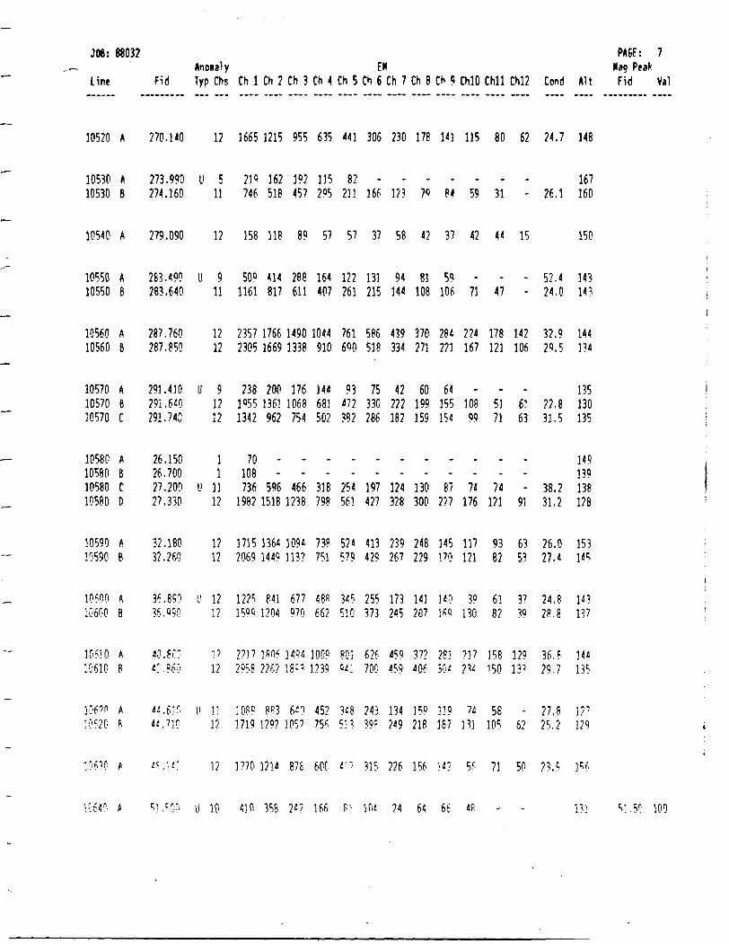
J08: 88032 PAGF: 7Anoialy EH Nag Peak

Line Fid Typ Chs Ch l Ch 2 Ch 3 Ch t C h 5 Ch 6 Ch 7 Ch 8 Ch 9 ChlO Chll Chl2 Cemd Alt Fid Val

10520 A 270.140 12 1665 1215 955 635 441 306 230 178 141 115 80 62 24.7 148

10530 A 273.990 U 5 2! a 162 192 115 82 - - - - - - - 16710530 B 274.160 11 746 518 457 2^5 21! 166 l?? 70 84 59 31 - 26.1 160

10540 A 279.090 12 158 118 89 57 57 37 58 42 37 42 44 15 150

10550 A 283.490 U 9 509 414 288 164 122 131 94 81 59 - - - 52.4 143 10550 B 283.640 11 1161 817 611 407 261 215 144 108 106 71 47 - 24.0 14?

10560 A 287.760 12 2357 1766 1490 1044 761 586 439 370 284 2?4 178 142 32.9 144 10560 B 287.850 12 2305 1669 1338 910 600 518 334 271 221 167 121 106 29.5 134

10570 A 291.410 U 9 238 200 176 144 93 75 42 60 64 - - - 13510570 B 291.640 12 1Q55 1361 1068 683 472 330 222 199 155 108 51 61 22.8 13010570 C 291.740 12 1342 962 754 502 382 286 182 159 15* 99 71 63 31.5 135

10580 A 26.150 l 70 - - - - - - - - - - - 14910580 B 26.700 l 108 - - - - - - - - - - - 13910580 C 27.200 U 11 736 596 466 318 254 197 124 130 87 74 74 - 38.2 13810580 D 27.330 12 1982 1518 1238 798 56! 427 328 300 227 176 121 91 31,2 128

10590 A 32.180 12 1715 1364 109' 738 524 413 239 248 145 117 93 63 26.0 15310590 B 32.260 12 2069 144? 113? 751 579 429 267 229 !?0 121 82 53 27.4 145

10600 A 36.890 U 12 1225 841 677 48" 345 255 173 141 W W 6 1 3? 24,8 W10600 B 36.Q90 l? 159C 1204 P70 662 510 373 245 207 169 130 82 3Q 28.8 137

10610 A 10610 B

40.80" l? 2717 ISO? 14P4 lOOO pni 626 459 37? 28J 217 158 129 36.8 141 '0.86'; 12 2958226218^1239 ^i 700 *59 406.50' 234 150 13* 29,7 135

1062n A u .W U li 10? 0 8*3 6^0 45? 3^8 243 134 159 11? 74 58 - 27.8 l/ 7 :0620 K t t.i]f. l ? 1719 129? 105? 75* 5:3 m 249 218 187 231 105 6? 25.2 1?9

1? 1770 1214 876 60C 4;7 315 226 156 *4? 56 71 50 23.9

iC64r- A u 10 4]D 358 2'? 166 f) KK 24 64 66 4? 13! 100

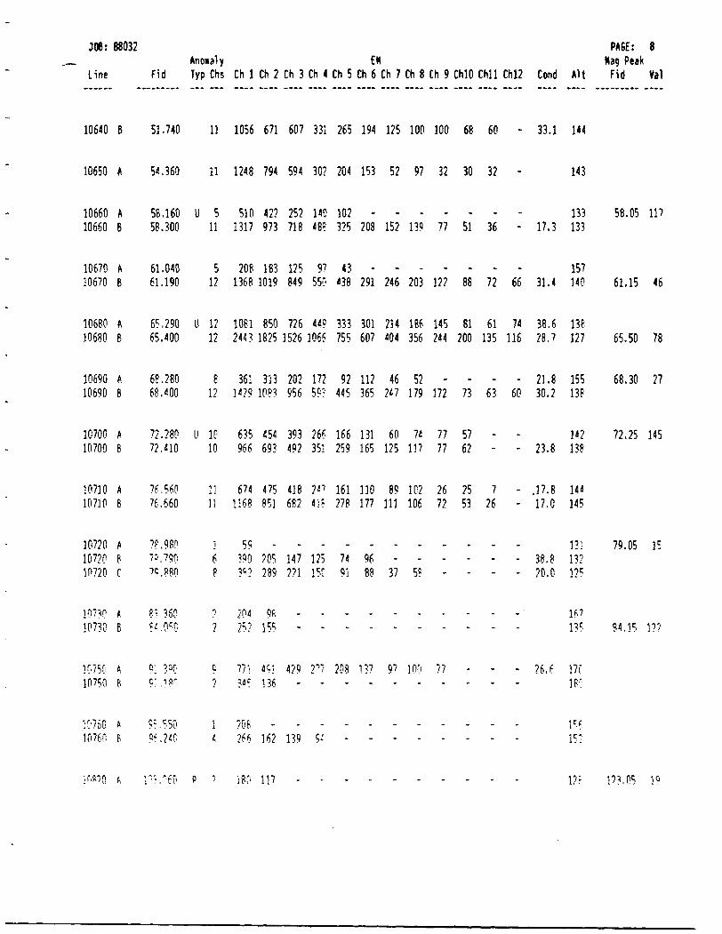
so'tLil 081 i d

;6 bel 2913*2 'd U9iOl * 09iGl

•Jitii Out to tit 802 ii2 bZIr i57 iii D Jot lo 1 O

del Sf'?6

51 50'6i

•HiM

tfl2EIitl

5*1?*l

-

~

0'02 -8'8E -

071 - 9' LI' -

-

"* " ™ ~ ~ ~

- - - 85 iE 88- - - - - 96

92 ES 2i 901 III iili 52 92 201 68 Oil

-. . .

16 051 122*i S21 i*l

8i2 jl* 289191 LJi 81*

bilS6

682S02

158Si*

i^im

citObt65

89H*i9

cL

j9r

illi

OSO'

09 i

088'Obi'u86'

099'G9S'

?iis

3tcidi

9i9i

g*

j9\/

9V

OEiOiOiiOl

02iUl02iOl02iOl

OUOlOUOl

SHZ9 ii ill Sil 591 652 ISE 26* i69 996 01 Olfr'Zi 8 OOiOl iS ii ?i 09 KI 991 99^ E6E fSJ Si9 Gl O m'lL i OOiOl

LI OE'89

8i OS'S9

8EI TOE 09 S9 Ei Zil 6il Lil 59S SSl 8' [Z - - - - ZS 9* III

ci5 956 HOI 6tol il lil m EtE I9E 8

Lil L'tt 911 SEl OOZ WZ 9SE ^ i09 55i 9901 3EI 9'8E W 19 18 SH 981 HZ WE EEE 6^

08Z'39

EN2 21 00?'59 OS8 1301 ZI n 06Z'i9

0690106901

9 08901 i 08901

SI'19ftE 99162 8E* 055 6N 6101 89EI li 06l'l9 9 Oi90l - Efr i6 521 E8I 802 S OHTW V Oi90l

ill SO'85EEI i' LI - 9E IS ii bit 251 802 S2EEEI - - - - - - - 201

8li Ei6 ilEI li OOE'85 9 09901 252 22^ 015 S n 09l'8S V 09901

2E OS 2E i6 25 ESI *02 20E *6Sli 09E'fS05901

Ml TEE - 09 89 001 001 521 MI 592 IEE i09 Ii9 9501 li Ofri'lS 9 OC901

PU l IV PUOO 2143 1143 0143 6 43 8 43 i 43 9 43 S 43 M3 E 43 l 43 l 43

8 :

ptj

2E088 :

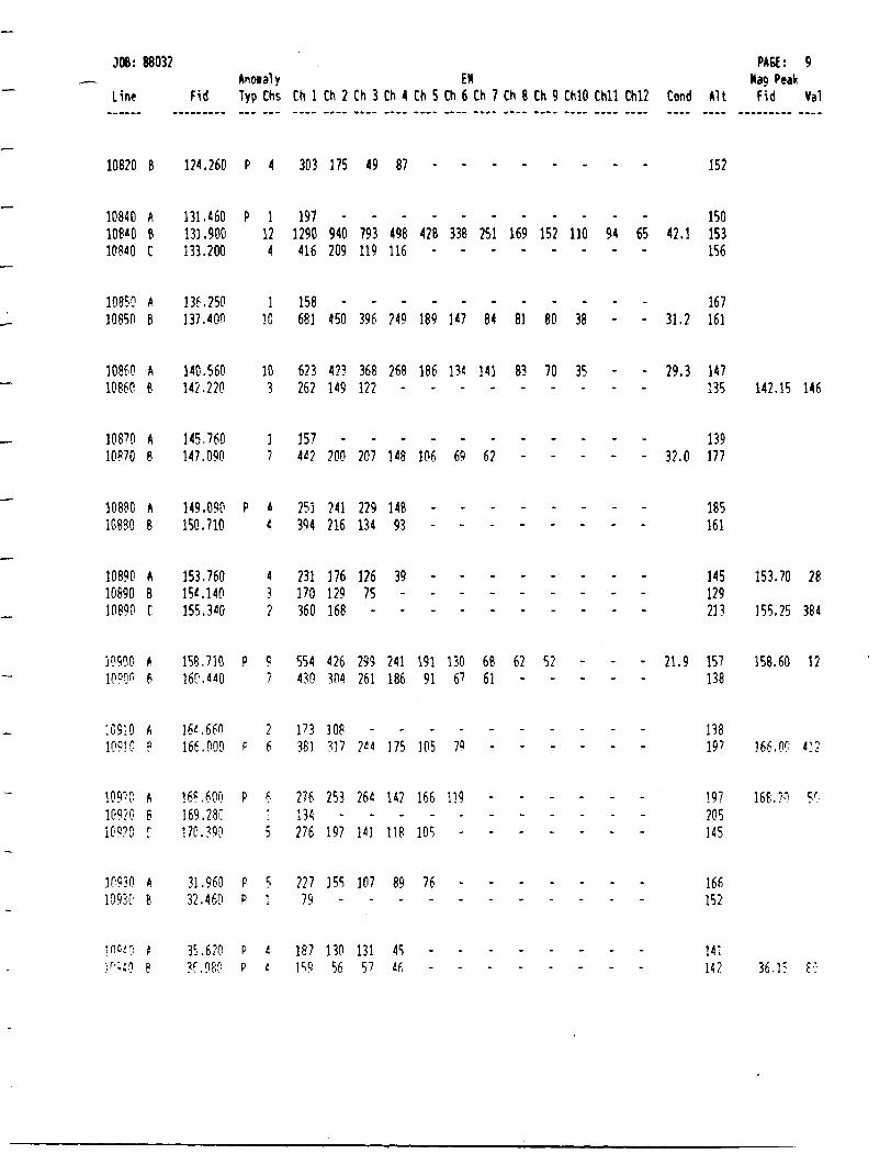
JOB: 88032 PAGE: 9Anofldly EN Nag Peak

Line Fid Typ Chs Ch l Ch 2 Ch 3 Ch 4 Ch 5 Ch 6 Ch 7 Ch 8 Ch 9 ChlO Chll Chl2 Cond Alt Fid Val

10820 B 124.260 P 4 303 175 49 87 - - - - - - - - 152

10840 A 131.460 P l 197 - - - - - - - - - - - 15010840 B 131.900 12 1290 940 793 498 428 338 251 169 152 110 94 65 42.1 15310840 C 333.200 4 416 209 119 116 - - - - - - - - 156

10850 A 136.250 l 158 - - - - - - - - - - - 16710850 B 137.400 10 681 450 396 249 189 147 84 81 80 38 - - 31.2 161

10860 A 140.560 10 623 4?? 368 268 186 131 141 83 70 35 - - 29.3 14710860 B 342.220 3 262 149 122 - - - - - - - - - 135 142.15 146

10870 A 145.760 l 157 - - - - - - - - - - - 13910870 B 347.090 7 442 200 207 148 106 69 62 - - - - - 32.0 177

10880 A 149.090 P 4 251 241 229 148 10880 B 150.710 4 394 216 134 93

185161

10890 A 153.760 4 231 176 126 3910890 B 154.140 3 170 129 75 -10890 C 155.340 2 360 168 - -

145 153.70 28129213 155.25 384

10900 A 6

158.710 P S 554 426 299 241 191 130 68 62 52 160.440 7 430 304 261 186 91 67 63 - -

21.9 157 158.60 12138

10910 A 36i.660 2 1?3 108 10910 P 166.000 P 6 38] 337

10970 A10920 B10920 C

165.600 P f-165. 280 3!70.?90 5

175 105 79

276 253 264 142 166134 - - - -276 197 341 118 105

138197

197205145

366.00 41?

168. ?0 5 r'

30930 A 10930 B

31.960 P 5 32.460 P l

227 155 107 89 7679 - - - -

166152

35.6?0 P 4 187 130 131 45 36.060 p t 1 59 56 57 46

341 K? 36. 3 C'

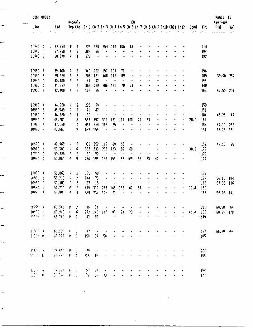
JOB:

Lin*

109*0109*010940

1095010950109501095010950

1096C1096010960109601096010960

30970109^0lOP'G109??

109irICWJ109=01P95-!I1P?:0

;r g; rio c: :1'"- r"1

1:0'!1:0:''

11 f:

110"

: i f "

8803]

cf)F

ABCDE

ABCDif

ABCD

ABroE

Api

AR

Ap

AR

?

Fid

. 37.38037.79038.040

39.46039.96040.40041.59042.400

44.96045.54046.26046.78047.06047.660

49.96050.38050.78052.060

56.06056.21057.30057.7105^.990

60.51060.94062.740

6S.tOrr.7.7QO

7S.59?77. ^ri

70 z. ? n8C , i' ; fi

AnoiTyp

ppp

pppp

ppP

pppp

ppppp

Ppp

Pp

Pp

pp

ia1y Chs

621

55262

221842

5629

22274

262

15

1?

13

Ch 1

525383372

34020644

363106

2257130

567467683

308362

30286

135144

57449369

46?724?

47159

70m

5?7?

Ch?

33096

26218142

22015

9947

397264159

252233

52193

907515

319237

54143

15

80

15

3565

EM Ch 3 Ch 4 Ch 5 Ch 6 Ch 7 Ch 8 Ch 9 ChlO C

254 164 106 68 - - - -.

197 104 70 - - - - -168 116 89 - - - - -

.206 130 70 73 - - - ---------

.

.

302 171 117 100 72 53 - -165 65 - - - - - --w------

119 89 58 - - - - -233 123 82 69 - - - -

.156 153 88 109 66 73 41 -

.

.

.273 165 132 62 54 - - -146 71 - - - - - -

.11? 95 94 70--------

59 - - - - - - -

-

.30 - - - - - - -

:hll Chl2 Cond Alt

- - 214- - 194- - 192

- - 196- - 209- - 198- - 140- - 165

- - 150- - 151

104184- - 28.0 184- - 184- - 151

- - 159- - 30.2 179- - 179- - 124

- - 173- - 199- - 166- - 17.4 180- - 168

- - 211- 46.4 183

- - - 149

107J?'185

- - 20?- - 185

19?- - 177

PA6I Nag f

Fid

39.

42.

46.

47.47.

49.

56.57.

58.

60.60.

66.

r t'eak

90

50

25

1075

15

1535

05

5085

70

10

Val

257

201

47

262131

28

184136

141

54178

?04

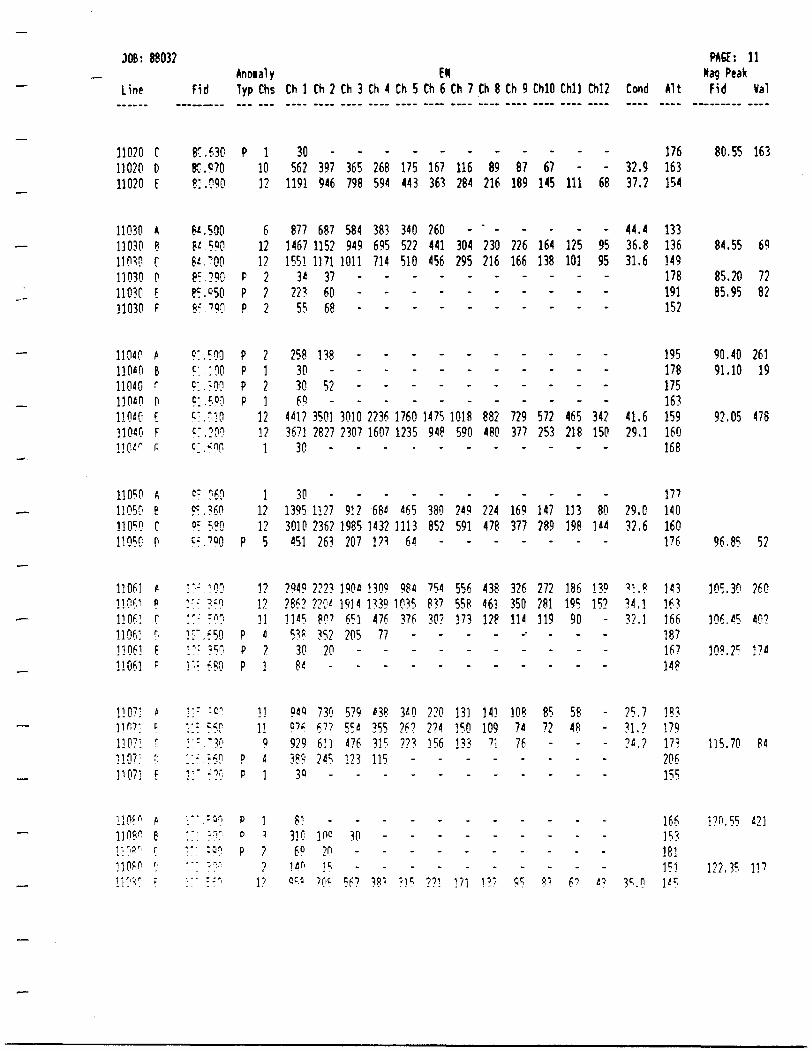
JOB: 88032

Line

11020 C11020 D11020 E

11030 A11030 R11030 f11030 D11030 E11030 F

11040 A11040 e11040 r110*0 D110*0 E110*0 Fi i ft jt 1*1 r

11050 A11050 Enow r11050 P

11061 (ino? 1 P11061 C1106: D11061 F11061 F

1107; A11 rt?! t1107; r1107: fi11071 f

* 1 '-. r

11080 Br.r,9r. rnew ^lii'v ;

Fid

K. 6308C.970K. 590

8*.5008* 590fi. "008: ,?90P!. 0508-' 7?n

9:. 590C' /Ipc* i on91.50*1c " ," 1.0"r. 209C " t flfl

. . i .'D*95.360o: 580?:."0

r.-- -n-,!'-' .369:' : W9l ".650:":: '50i "i K oni ' * H f,i i

v :c*T s^p

:1 ."30:'. :6P1 " - ^ '

- - - ; r,- - : -.r

•:: :?o- . : ' ;

" " * r ^ H

Anoial y Typ Chs

P 11012

6121?

P 2P 2P 2

P 2P 1P 2P 1

121?

1

11?12

P 5

1?1?11

P 4P 2P 1

1111

0P 4P 1

P 1P qP ?

21?

Ch 1 Ch 2

30 -562 397

1191 946

877 6871467 11521551 1171

34 37223 60

55 68

258 13830 -30 52COPH

4*1? 35013671 2627

30 -

30 -1395 11273010 2362

451 263

294? 2223286? 220'11*5 80 ?

53S 35?30 20Q j

ojo 73007S f ll929 631389 W

30 .

RI310 l nc

6 C 201* r' 15QC.C 7fit

Ch 3 Ch 4

365 268798 594

584 383949 695

1011 714---

-

-

3010 22362307 1607

912 6841985 1432207 123

1904 13091914 133?

651 476205 77

-

579 4385^* ^55476 31 c'123 115

30 -

-5F7 38*

Ch5

175443

340522510

--*

^

-

17601235

4651113

64

9841035

376--

3*026?223

-

.--

?15

ENCh 6 Ch 7

167 116363 284

260 -441 304456 295

--~ *

— .

-

1475 1018948 590

380 249852 591

-

754 556837 55830? 173

--

220 131224 150156 133

-

.--

??1 171

Ch8

89216

-

230216

--~

.

-

882480

224478

-

438461128

--

141109

71.-

.--

1??

Ch 9 ChlO

87 67189 145

— .

226 164166 138

--" "

- .

-

729 572377 253

169 147377 289

-

326 272350 28111* 119-~

-

108 8574 7276 -

-

.--

95 w

Chll Chl2

-111 68

- ^

125 95101 95

--"" "

. .

-

465 342218 150

113 80198 1*4

-

186 13?195 15?

90 ---

58 -48 -

-

.--

6? t 1)

Cond

32.937.2

44.436.831.6

41.629.1

29.032.6

-11 .a3*.l32.1

25,731.?

3^.0

Alt

176163154

13313614917819115?

19517ftI/O1751631591601CO100

177140160176

1431631661871674 J ft14r

183179173206155

1661531811511*5

PAGE: 11Nag Peak

Fid Val

80.55 163

84.55 69

85.20 7285.95 82

90.40 26191.10 19

92.05 478

96.85 52

105.30 260

106.15 40?

108. 2^ 174

115.70 8*

120.55 421

122.35 117

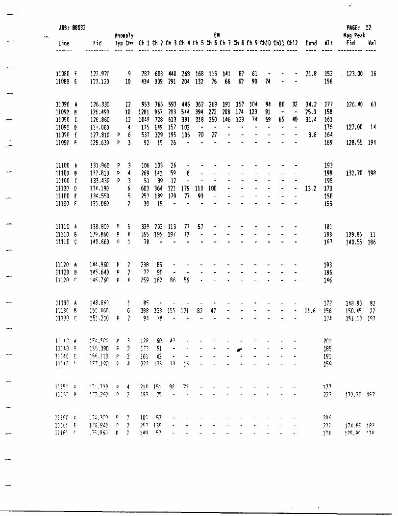
oil 06 'ailtd l aS'Pil

iBl OE'Zil

ibl ul'lbl22 b* '0517 Q fi(* ' 0 h T Co UO uPl

981 SS'Onli 58'6El

861 Oi'ZEl

?6l SS'82l

n 00721

E9 Ofr'921

91 00'E2l '

feilie 'M

t22til

651161581202

lil951 9'll -2il

9H981E61

L j l881181

SSlOSlOil Z'EI -S61661E61

691m 8'E -9il191 r IE n851 E'S2 -iil 2'fE 2E

9SIZSl I'll -

--— - — — - ~™ ~~

.........

tt 36

- - - - - - - 91 U-

* .it

- - . . . . . - .

it 28 121 551

- - - - - - - 9S 98-— ™ — — " ~ m ~~

ii i6l- - - - - - iS ii Ell

--.------

- - - - - - E6 ii 6il- - - - - 001 Oil ttl IZE- - - - - - - - 21- - - - - - - 8 6S. . . . . . . - 9Z

- - - - - - - - 92- - - - - LI Oi 901 561- - - - - - - 201 iSlS9 65 H ill 9H OS2 81E 16E E19- 16 E21 ttl 802 2i2 m MS E6i08 frb m iSl 161 692 29E 9kt E6S

- tt 06 29 99 9i ZEl WZ 162- - 19 i8 in Sil 891 892 m

tsoEli5

St151

5212?tb09

iLESE

2910658

561202

51681WE6Eintfl l

SI6ZE6*182ii9699i

60EE09

belCaZsOl

titj 12

LLL101tit321

tb88E - a30

652iim

p/ 9tS9E6EE

OE252E09IS692901

26iESSil6?0l1821ES6

^

lLL

ci?

1lii

l9l

tLl

l1S

2S9EpE

E9t210121

016

dJa

ad

dddd

d

ddd

ddd

ddd

dd

096 jVb'

GOE

0*2'ut i'

OD r OH1G6E1cos-

012'09fr' ' 00 *^

09i'W096'

uyy 098'008'

090'OSS'061'OE*'0181096'

OE9'018'090'098'06*'OEE'

021'Oi6'

'1;i-"

"Ji.1::.

L' t•li.:

;;i l?5".bil •1,1

liloil . . -8

ynb?l7Fl

Of LOtISE l

btililFEIEElcElIt l

82:tZlttl921921921

iZl221

jdi

a7

•j

jii

jdg

j

a*

39'

j30J9i

t3039V

9\

J9llij in 1 1091 i i

.bill

.bill

jnnon nGvtllUPUI

uEtllOElllOElll

0211102111OZlll

OllllOllllOllll

OOlllOOlllOOlllOOlllOOlllOOlll

060110601106011ObOU060 li06011

0801108011

PUUV PU03 2143 1143 0143 6 43 8 43 i 43 9 43 S 43 M3 E 43 2 43 l 43 sq3 dXiH3 ^ewuv

PH

21 :2E088 :90f

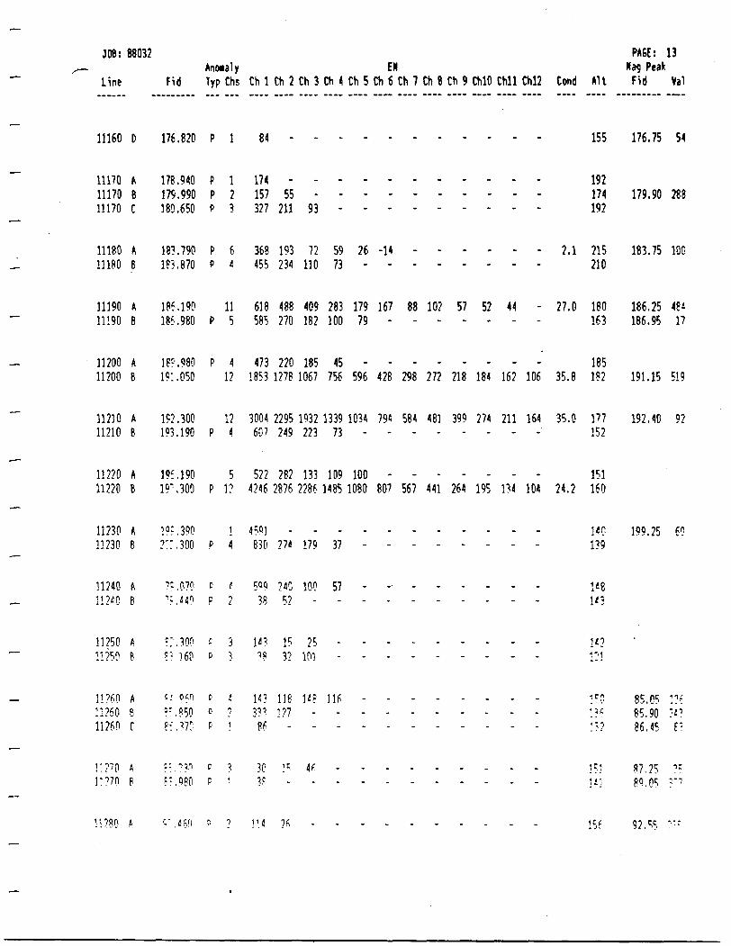
JOB:

Line

11160

111701117011170

1118011180

8803:

D

A8C

Ae

2

Fi

176

1701 r P

179180

1831??

d

07fi.OiU

.940

.990

.650

.790

.870

Ann Typ

P

PPP

PP

laly Chs

1

123

64

Ch 1

0484

174157327

368455

Ch2

55211

193234

Ch 3 (

-93

72110

EM :h 4 Ch 5 Ch 6 Ch 7 Ch 8 C

.- — m. . -

59 26 -14 - -73 - - - -

h 9 ChlO Chll Chl2 Com) AU

- - - - 155

- - - - 192- - - - 174- - - - 192

- - - - 2.1 215- - - - 210

PAGE: 13 Nag Peak Fid Val

176.75 54

179.90 288

183.75 10D

11190 A 186.190 11 618 488 409 283 179 167 88 102 57 52 44 - 27.0 180 186.25 48411190 B 186.980 P 5 585 270 182 100 79 - - - - - - - 163 186.95 l?

11200 A m . 980 P 4 473 220 185 45 - - - - - - - - 18511200 B 191.050 12 185312781067 756 596 428 298 272 218 184 162 106 35.8 182 191.15 519

11210 A 192.300 12 3004 2295 1932 1339 1034 794 584 481 399 274 211 164 35.0 1?7 192.40 9211210 B 193.190 P 4 607 249 223 73 - - - - - - - - 152

13220 A 195.190 5 522 282 133 109 100 - - - - - - - 15111220 B 19".300 P 3? 4246 2876 2286 1485 1080 807 567 441 264 195 134 104 24.2 160

11230 A l Q?.390 l 4513 - - - 11230 B 7:^.300 P 4 630 274 179 37

199.25 60

31240 A 11?40 B

?: .0?0 P ' 5oci 240 100 57 ".'40 P 2 38 52

11250 A 11250 B

f :.?0' P 3 ? : 360 D 3

15 25 M. 1 03

11?60 A s: ofn c- t 1 43 ne 3*8 31611760 6 s : .?50 D 7 33? 37713260 C E:.*7C P 1 86 - - -

85.05 17:85.90 5*?86.45 F-

31270 A 13770 B

31280 A

? : .980 P 130 35 46

li] 80.05

!5f 92.55

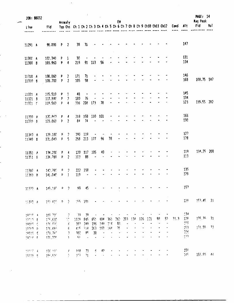
o\ **—

JD u

.

CN

l*-H.CtJososL

J

CD

Sr**CJ

u vo55LO,cjrC-*

roS^^"5

g ^cr

^s

TD

Lk.

at

iiiiiiiiiiro00

ror-Ma-

gCD

g^* — iS

II

II

III

II

li

II

II

li

li

III

II

II

li

1 '

li

li

III

II

II

' '

'1

li

II

III

II

II

II

II

II

II

III

II

li

li

1 *

li

li

III

II

II

II

' 1

li

1 1

III

li

II

II

li

|l

li

III

II

1 O

O

II

II

r^~

t VO

1

* 1

* O

O

' — *

1 1

VO

C

D

1 1

1to

r*~

CD

cr.

^r

1 O

O

II

1 l

OO

C

D

1 ir--

LO

1

li

^ — t

1 — 1

* — t

* — "

* — *

i *—

* ,—

t oo i

vo oo

00^3

- cr.ro

r-- o

o

20. '

ON

r-** LO

r*- CD

LO r^

*—

* *—

* *—

* oo LO

C^

ON

,—

( L

O

OO

C

D

VO

O

O

^3

CD

O

O

CD

O

o

O-si

O^

ro

*— *

r— CD

^r oo oo

-— *

oo cr.

LO

rsi CD rvi *—

t cxj

*— i

* — t

t — ( ro

rsi

* — i rsi

* — t

* — i

^si ^ — i

, — t

^j-

rvj

cvj , —

i c

*^. ^r

^i'

Ox(

f*--* LO

^

CN.I O

"- * —

i

o-O

- cud.

CL.C

L.O

. o

. ou

o-o

- o

-ou

C

IQ.

cr*

CD

C

D

CD

C

D

CD

c^.

c-.

CD

c^

cz. c-i

c:.

t,-- c:-

^

vo

vo

C

D

4 — i

O-.

vo

vi:*

vo

oo

*a

o

o

oo

o^1

*r

ro

Cfi

CD

*^*

LO

LO

LO

C* -

CD

* —

' C

D

r"s*1' r*-

n*

Ci

S S

S

S

iC ^

o^ fC

^i oo' ^.o

o

S- s?

-^

(O

-*C

OO

-*

t G

O

*^.

-*C

CO

-^ca

4.0

LJ

^C

-OL

.

CD

C

D

CD

C

D

,-j ^

,-H

cr,

CD

C

D cr.

^j ^

c^ c:

oo'

oo

oo

oo

o

o

oo

r*-. o*"i

ro

oo

oo

OO

o

o

O^'

o-~, —

— t

v ——

* i —

— l

*— *

l ——

1 1 —

— 1

^ ——

( ' —

— '

* ——

1 *~

*

* ——

' * —

— '

* ——

' ' —

— *

*~

1 l

l O

*: l

1 1

l

1 1

1 O

C

1 1

l 1

oo

1 1

1 1 —

1 1

1 1

1

1 l

l V

*D

1 1

1 l

1 1

t -Q

1

1 1

1

f- 1

1 1

1 (-"-l

1 1

1 1

1 1

1 l*

- .1 00

VC

i l

1vo

co

r—c^*

' '

' C

S ^-

^r

' '

(TrJ V

-i ^-;

i i

i *a

vi

c:-

i i

oo

vr

vo

i i

i r~

- vo

m

oo

i

LO

* —

— '

O -

LJ"

1 *D

. "3

l-T

' (

^-* oo

rsi

,'-,

cr.

LT r-

r- .i o

,- .

or.

ij-

C* i

*-^-j C

"'- r

' vi^-

yf' f"^"'

r—-

d

0-

c

c. - c

c.^

i^ -

-j. *-

' t:-

•— -

*a o-

M/.'

O

^j

r-- r-

i^ t^i

^ '^- ^ ^ i^.

^1

^

-' ^ ^ ^

L*,

LL.

C'.^

c.'

*^ c: -

--r ci

c:

o.

O7"-

ori

^L - c" -

CTJ cr '

*z. ' c:

*- -. t- -

O -

i J' O

C

* O

O

"

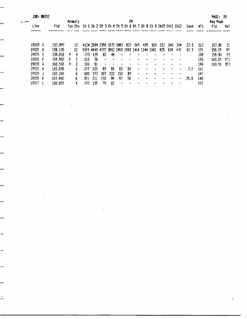
JOB: 88032

Line

19020 C19020 D19020 E19020 F19020 6190?0 H19020 J19020 K19020 L

Fid

157.890158.120158.810159.960160.560163.030163.260163.460163.830

Anoialy Typ Chs

1212

P 4P 2P 2

6664

Ch 1 Ch 2

4124 29895915 4849

173 135110 78106 51277 225600 373351 211197 135

Ch 3 Ch 4

2396 15724272 3092

82 48--

89 89307 222150 99

79 62

EN Ch 5 Ch 6

1083 8222459 1993

---

63 54150 8997 58

-

Ch7

5651464

-------

Ch 8 Ch 9

409 3091244 1041

-------

ChlO Chll Chl2

212 146 104825 639 476

.

.-....

Cond

22.542.3

7.1

25.9

Alt

112121108130196161147140157

PAGE: 15Nag Peak

Fid Val

157.80 20158.15 8?158.90 E3160.00 5C5160.55 353

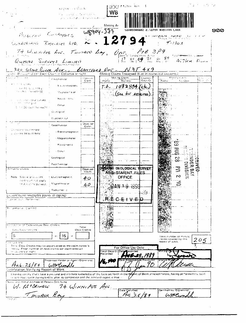
900

Ri :'ji,i:s''.:u i-'or' Eaci. Cliirri i ri Columns at riijlit Mining Claims Traversed (List in numerical

uoned at the claim holder's

Tot?i; n-jmher ot mimnq claims covered by ihis reoort of work. 2^5

Certification Verifying Report of Work

^corded Holder or Agent (SignaujreJJ

j l hereby remf y i hat l have a personal and intimme knowledge of tl'ti fdcts set forth in the R^rort o f Work annexed hereto, having performpd thu workj (H ivit'i-^sse-i 5;nr;e during and/oi alter its completion and the jnnex^d report is true. [f i

[rvj.i'Tin ,inti ^ott.31 Ackiress of Person Cetiifylng

l ^* "' * * * . .. ——— -, . . . . -, * ,-i..-.te Certified

/we 'l* /X fed by (Signature)

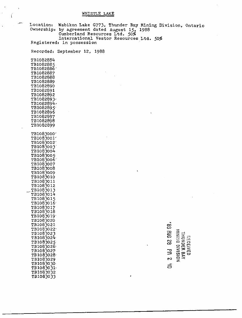
WHISTLE LAKE

Location: Wabikon Lake G773, Thunder Bay Mining Division, Ontario Ownership: by agreement dated August 15, 1988

Cumberland Resources Ltd. 50#International Vestor Resources Ltd.

Registered: in possession

Recorded: September 12, 1988

TB1082884TB1082885TB1082886-TB1082887TB1082888TB1082889TB1082890TB1082891TB1082892TB1082893-

TB1082895' TB1082896" TB1082897 TB1082898TB1082899

TB1083000-TB1083001"TB1083002'TB1083003TB1083004TB1083005TB1083006'TB108300?TB1083008TB1083009TB1083010TB1083011TB1083012

TB1083014TB1083015TB1083016-TB1083017TB1083018

TB1083020TB1083021 CD TB1083022- ^ 2: TB1083023 S ^ d TB108302^ ^ rr c TB1083025 So CT o TB1083026 ' 2 m Ej TB108302? 12 m TB1083028- 3 S2 5 0 TB1083029 ro g -* TB1083030 .c TB 10 830 3 1- 0 TB1083032 TB1083033

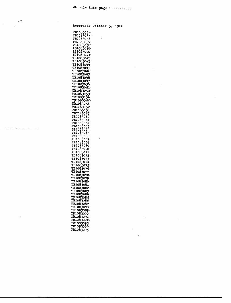
Whistle Lake page 2.

Recordedi October 5, 1988

TB1083034TB1083035TB1083036TB1083037'TB1083038"TB1083039-1610830*40TB1083041-TB1083042TB 10830^3'TB10830W

TB1083046- TB108304? TB1083048

TB1083050TB1083051-TB1083052TB1083053TB1083054TB1083055TB1083056TB1083057TB1083058TB1083059TB1083060TB1083061TB1083062TB108306318108306^TB1083065TB1083066TB108306?TB1083068TB1083069TB1083070TB1083071TB1083072TB1083073

TB1083075 TB1083076 TB1083077 TB1083078 TB1083079 TB1083080 TB1083081

TB108308?TB1083084TB1083085TB1083086TB1083087-TB1083088TB1083089-TB1083090

TB1083092- TB1083093-

TB1083095

Whistle Lake page 3.......,

Recordedi October 31, 1988

TB1083393'

Recordedi October 14, 1988

TB1083400'161083*101'161083*102TB1083403TB1083404TB1083405TB1083406TB1083407

Recorded: October 25, 1988

TB1083479-TB1083480TB1083481 TB1083482 TB1083483

TB1083485 TB1083486 TB108348? TB1083488 TB 1083^89 TB1083490

Recorded: October 31, 1988

TB1085010- TB1085011- TB1085012 TB1085013

TB1085015 TB1085016 TB 10850 l 7 TB1085018 -TB1085019 TB 10 8 50 20 TB1085021 TB1085022 TB1085023 TB 108 50 24 TB1085025 TB1085026 TB1085027- TB1085028- TB1085029 TB1085030 TB1085031 TB1085032 TB1085033

TB1085036- TB1085037- TB1085038 TB1085039-

TB109261?TB1092616-TB1092619-TB1092620TB1092621-TB1092622-

Whistle Lake page 4.

TB1092642-TB1092643-'TB1092644TB1092645TB1092646TB1092647TB10 9 2 648TB1092649TB1092650TB1092651TB1092652TB1092653TB1092654TB1092655TB1092656-TB1092657-TB1092658-TB1092659TB1092660-TB1092661-

TB1092679- TB1092680- TB1092681- TB1092682- TB1092683- TB1092684- TB1092685- TB1092686-

TB1092688- TB1092689. TB1092690- TB1092691- TB1092692-

TB1092694- TB1092695. TB1092696-

A 1

H

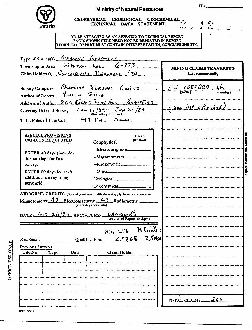
y-ntario

Ministry of Natural Resources

GEOPHYSICAL - GEOLOGICAL - GEOCHEMICAL TECHNICAL DATA STATEMENT

File.

l 9-V, 7*W

TO BE ATTACHED AS AN APPENDIX TO TECHNICAL REPORTFACTS SHOWN HERE NEED NOT BE REPEATED IN REPORT

TECHNICAL REPORT MUST CONTAIN INTERPRETATION, CONCLUSIONS ETC.

zoaCAD WuE u, o

Type of Survey(s).

Township or Area.

Claim Holder(s)

-77 '3

Survey Company _

Author of Report _

Address of Author 2-O O

Covering Dates of Survey.

Total Miles of Line Cut

(linecutting to office)

411 \t*A

SPECIAL PROVISIONSCREDITS REQUESTED

ENTER 40 days (includes line cutting) for first survey.ENTER 20 days for each additional survey using same grid.

DAYS-, . . , per claim. Geophysical

-Other

r.^rh^mir.1

AIRBORNE CREDITS (Special provision crediti do not apply to airborne surveyi)

Magnptomfter 40 Electromagnetic 4-Q(enter days per daira)

HATR. AJ&- 1 b jAuthor of Report or Agent

Res. Geol.. .Qualifications. 2. 9?

Previous Surveys File No. Type Date Claim Holder

MINING CLAIMS TRAVERSED List numerically

(prefix) (number)

4^J^.Jj^...^M..^:ffL^4^}..,

.5

Vl

TOTAL CLAIMS. 2.0Z

837 (5/79)

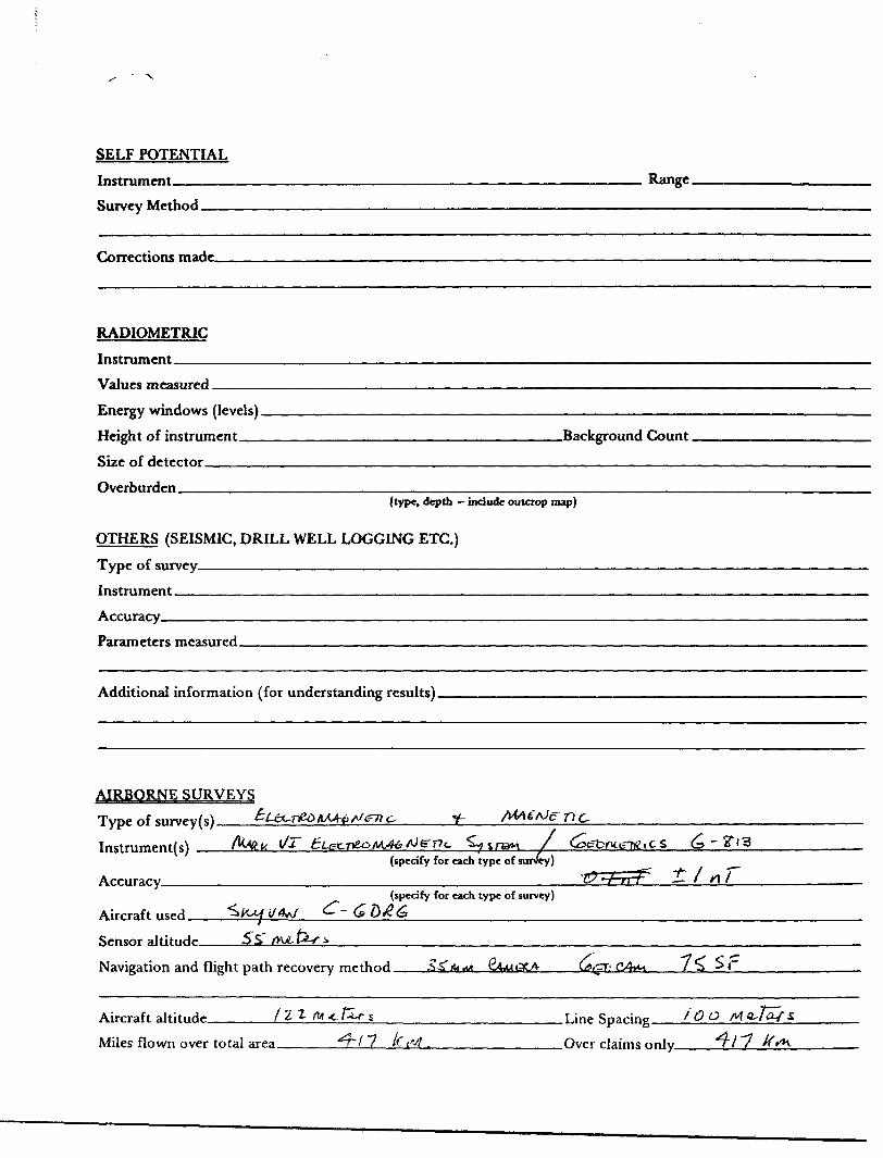
SELF POTENTIALInstrument———————————————————————————————————————— Range.Survey Method -—————————————————————————————————————————————

Corrections made.

RADIOMETRICInstrument———Values measured.Energy windows (levels) —-—-—————-——™——————————-—.-———.—.————Height of instrument______________________________Background Count. Size of detector—————————————————————————————————————————————Overburden --——..^-——————.——----—^———-—-——.^—-——.—----———--———..--

(type, depth — include outcrop map)

OTHERS (SEISMIC, DRILL WELL LOGGING ETC.) Type of survey——————--—.-—-——.^-.————————-Instrument -—————————^—.————.———-———.Accuracy————————————————————————Parameters measured.

Additional information (for understanding results).

AIRBORNE SURVEYSType of siirvpy(s) kUc.TdOnMretJfmc,-———t- flMitJcT\t,Instrument(s) fa** ^ Eu^T**MA0 AJtrPc "S^mn 7

(specify for each type of survey)

Accuracy _______________________________________ "^ -t-rr' ~ A l(specify for each type of survey)

Aircraft ..seH ^Kx (//W ^

Sensor altitnrfp 5s' AU. fer s

Navigation and flight path recovery method. 64wi3tA Cftt GXWoi /S

Aircraft altitude ______ /' 'i ™ *- ^ s __________________ Line Sparing f OOMiles flown over total area _____ T i 1 K f-4 . ____________ Over claims only ___ i l~7

Telephone (807) 344-6598

CumuziLand d\s,ioaiczi Jltd.

fjjid^^^:

74 W innipeg Avenue,THUNDER BAY, ONTARIO

P7B 3P9

zr- t*y tJ w-^a UMDS SECTION

RECEIVED~:07 l:

. ,y ' f

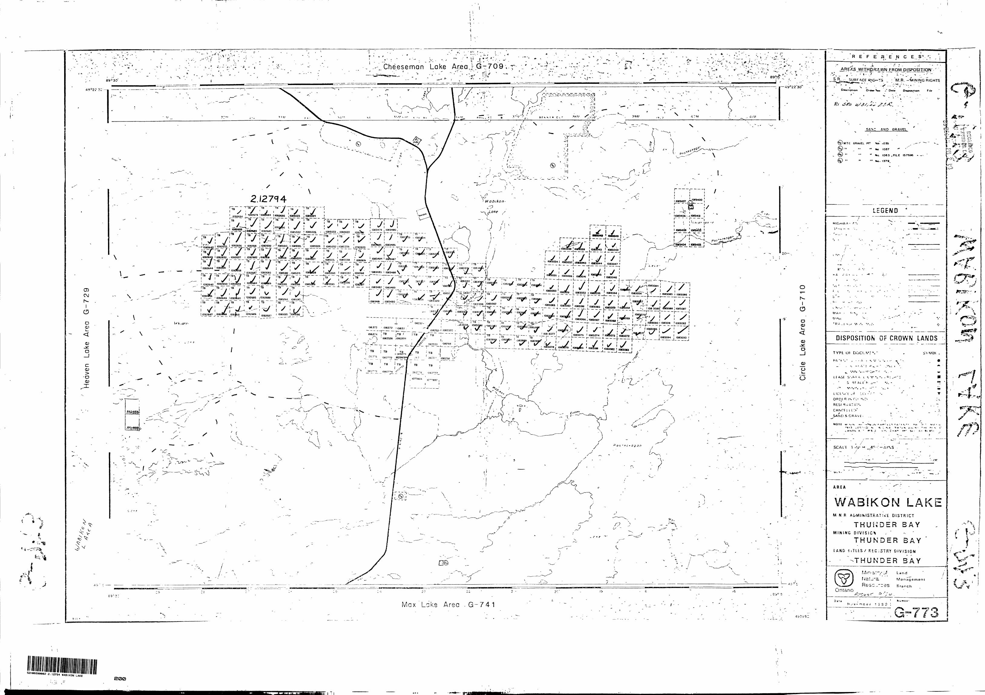
-t --.

vfcs '-4

REFERENCES

^Cheeseman Lake Area,G-709,.r yilIHP.Hl^\VN^R OMJP ISPOSITI ON - .T *- . " -. '

M:R. --MINING RJGHTS

,~ Dal* OitpoMtion File

SANC AND GRAVEL

MTC GRAVEL PIT -to .035 .-- '

1037 " ''

1063 .RLE 157596 - -

12794

i wf i 7 'MnMf l IOU04I I .r -.- n —j.—J——Jx

' i ^J—-r-1 ~ ' - ' * '

i *. l - l 108502? '1085025. - .JMSOSJ . 1032622 IQS^B. '

y y - / y"7jO__ __™ T TB "

:,^:T:^^ i^ "i^TytT:-/f-T-ryl^y-- - /'"--- ' ^ ^! i ' ' ' 1083050' y l " ' J ~\ V I 'M*KS X-losaoy -TB OBSC^T,""^^ 'TO~~~—rrs" ~ ~ V"*~ ~~^-r ~ — _ — — ' '— — - L 1?????2 ' '??*?? ioaso64 | l loeaose^•X-i^^'i -^ :-^ .;v ;-y y i yi'/ryry^V,^i^---^^^-"-^^-;,r --^..:^.j.r^j.^j~i ;-i. :^. :^\ '~

— —— — —l IO834B2 ! IO834BS

l 7" 7B

! y : ^1092649 11092*60 l '092685

ITB JTB i TB

i—' f .J loasoi j loaao^-' 11083/11

y ' j ~~ ']I^2-1--1 ^no^ J ^07, JTl: ^ JI0 4 j ^ i

•' y' . : x -l ., 7 y !" r~~ — ^ DISPOSITION Or CROWN LAMDS

L icf.rt ^' '-Ci --R IN r^i - '-.C'

RLSf Rv AT If:'.

CANCE 1 1 1: SAND s. GRAV{ -

NOTE M N.*. t.. -."i i 3 . f *i ' - D i.

L - W5

WABIKON LAKMMR ADMIMSTRA';*'E DISTRICT

THUNDER BAYMININGDIVISICH : * - "

THUNDER BAYIAND liTLtS/ RtS:STRY DIVISION

THUN? DER BAY

Max Lake Area . G-741

LAKE soo

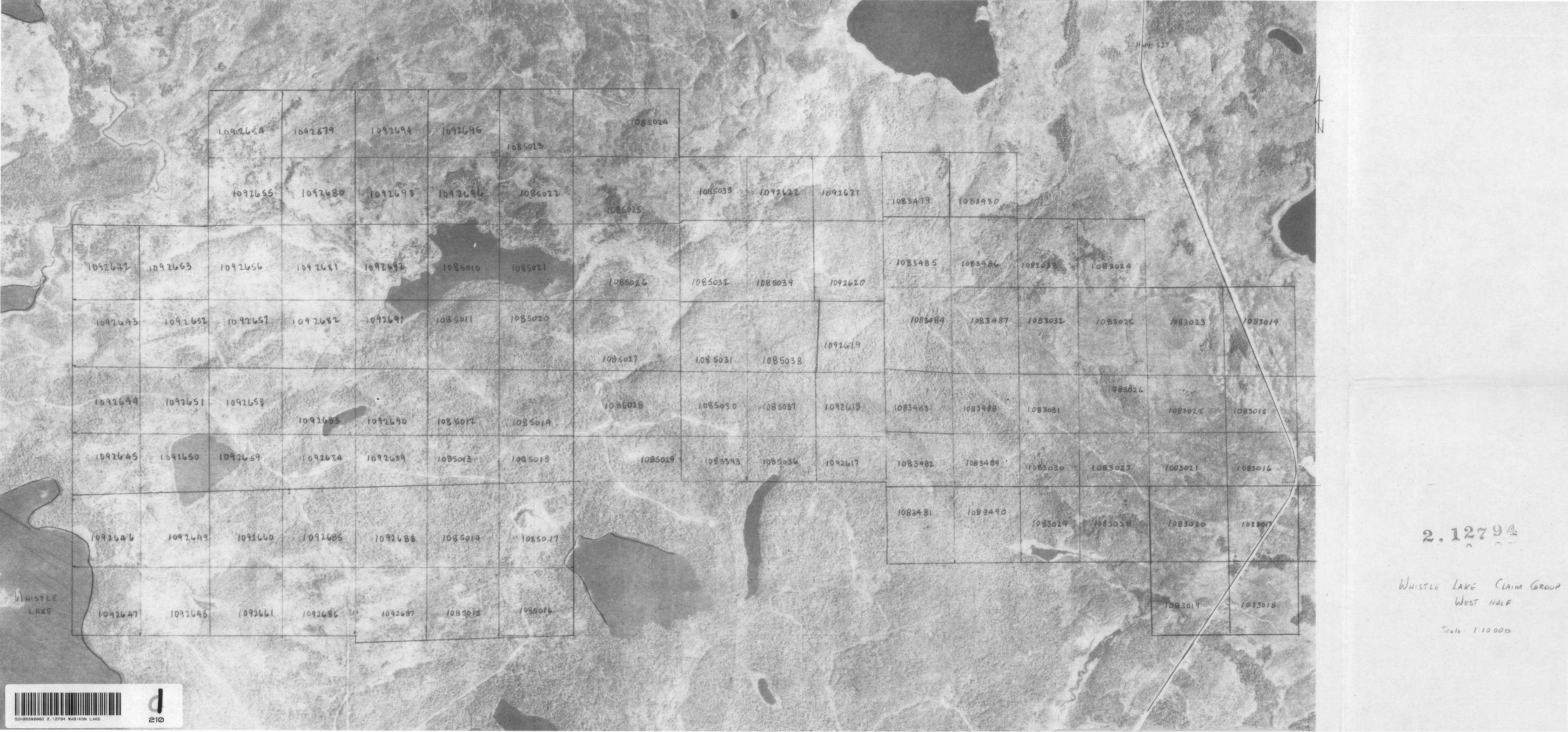
-x3 o w:

O^

oc*

'-it-J

k,];r

r*

Ocd^O

(O

O

t*r-00

03OCDcOO

S

lOOT^ 03

daea o

cr

03O

(AO\nCDo

O

r-INOt^

QQOrf)O m

oOo

(O

00or*CO

00o

Ci

traaQaa*

rfl00 O

cr o(O

i

e- f

-^.•' r"^i-jfe'"^

W^vr^

vv' ."-

1 "'.Bb

siS'1 V

'-. -' -i--if-''

'- .:

O\nO

H

OVI

afe O

Ci

c*r*oO

c*P

-TO

o-ol O

vOeo•V

i

Cf

O

O

l,jr

T*;

f

Os-

^

^

? 5

2L

O

^•y

__

^5

-^t. O

' t

J '

—fi:X

—

—

I -S

t

rK-

i4...

j,, ^

p^ "

^-- -

*\n

*

^

J

J

^

-J

-*

S

Hor

•*-c

i r

. ,, ....~*V

(5-ocO^^*yad-

••^.r" ^;.-,,

^28|

-a ^

A

Hcj-

O

?.

O^r*

-3TO.5r1

<T-

Dc^•^^r-**5-

O

_____L

—.L

r-*oro

O

(T*-3

S i

H•r"

O*o

vn COocflC

O

CD-^c-io

- O

VIo.(DOOP

-OCi

G~

O2 J

G.

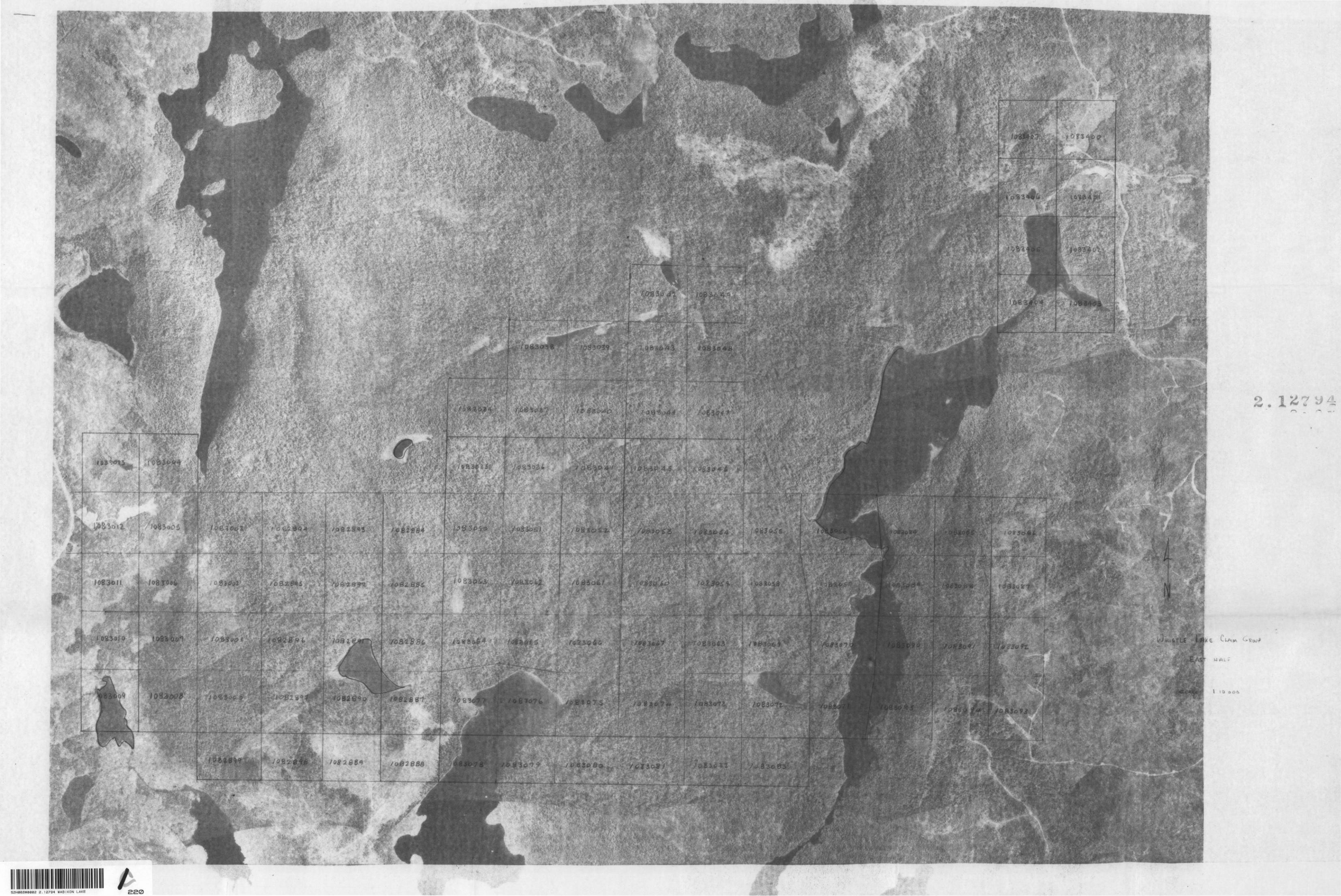
f 08 3o

•i '\ o "4 R

-S J/-4. JL ^

1

N

X W ' -*J O W

U AL ir

l t t) oDfi

B20

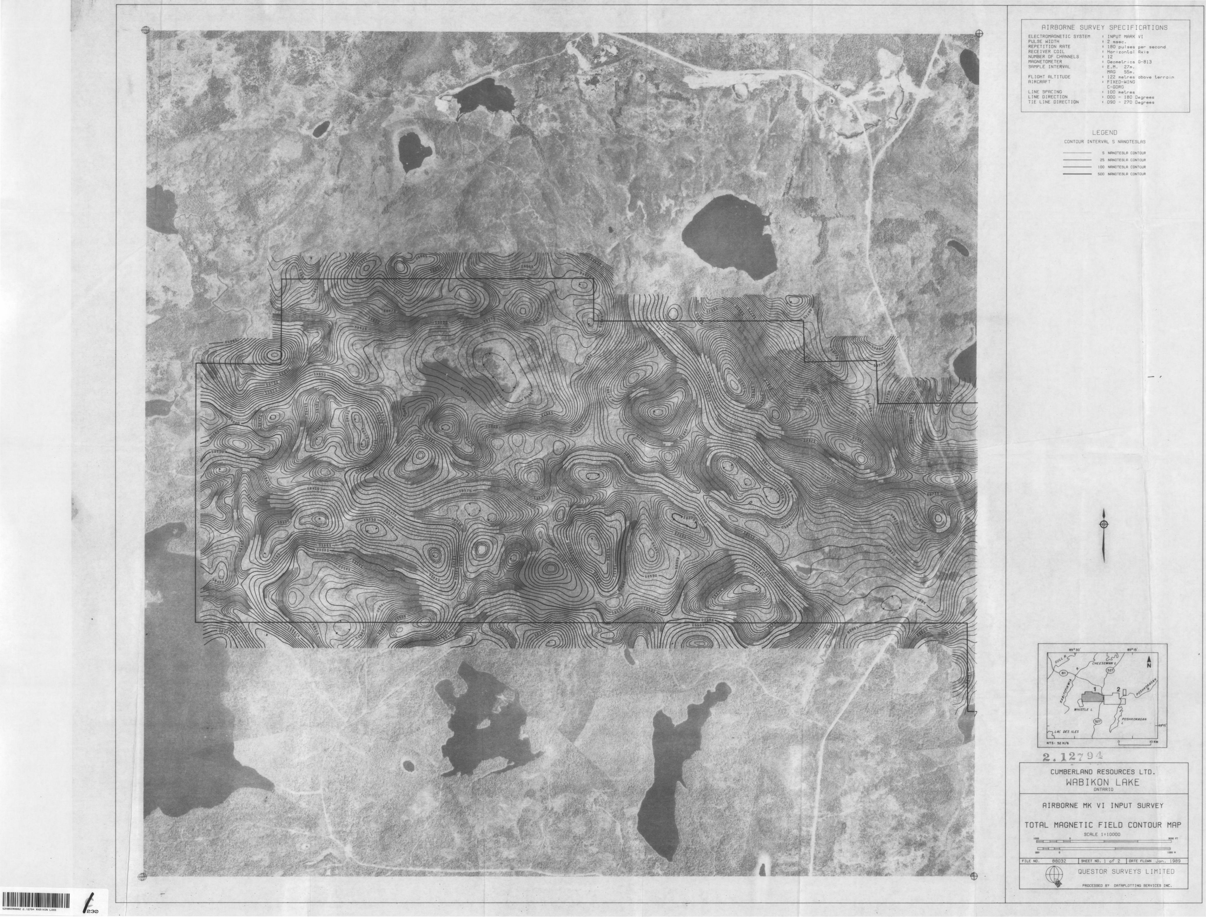
/330

7

RIRBORNE SURVEY SPECIFICRTI QMSELECTRQMRGNETIC SYSTEM PULSE WIDTH REPETITION RRTE RECEIVER COIL NUMBER OF CHRNNELSMflGNETOMETER SRMPLE INTERVRL

FLIGHT RLTITUDE RIRCRRFT

LINE SPRCING LINE DIRECTION TIE LINE DIRECTION

INPUT MRRK VI2 msec.180 pulses per secondHorlzontol Rx i s12Geometrics G-813E.M. 27m.MRG 55m.122 metres above terrainFIXED-WINGC-GDRG100 metres000 - 180 Degrees090 - 270 Degrees

LEGENDCONTOUR INTERVRL 5 NRNOTESLRS

5 NRNOTESLP C ONTOUR

25 NPNOTESLR CONTOUR

100 NRNOTESLfl C ONTOUR

500 NflNOTESLR CONTOUR

B9 0 30

CUMBERLRND RESOURCES LTD.

NRBIKON LRKEONTRRID

RIRBORNE MK VI INPUT SURVEY

TOTflL MRGNETIC FIELD CONTOUR MRPSCflLE 1 - 1 0000

1000 0 3000 FTFZZq ——— 1=1 ——— 1=3 —————————————————— l ^Z3 —————————————————— 1

1 —— 1=1 ——

ZOO

F^ ———————————————————— 1 10 1000 H

FILE NO. 88032 | SHEET NO. 1 of 2 DRTE FLOWN J an . 1989

\\ Q UESTOR SURVEYS LIMITED

^T PROCESSED BY DflTRPLOTTING SERVICES INC.

52H06SW0302 2 .12794 WABIKON LAKE

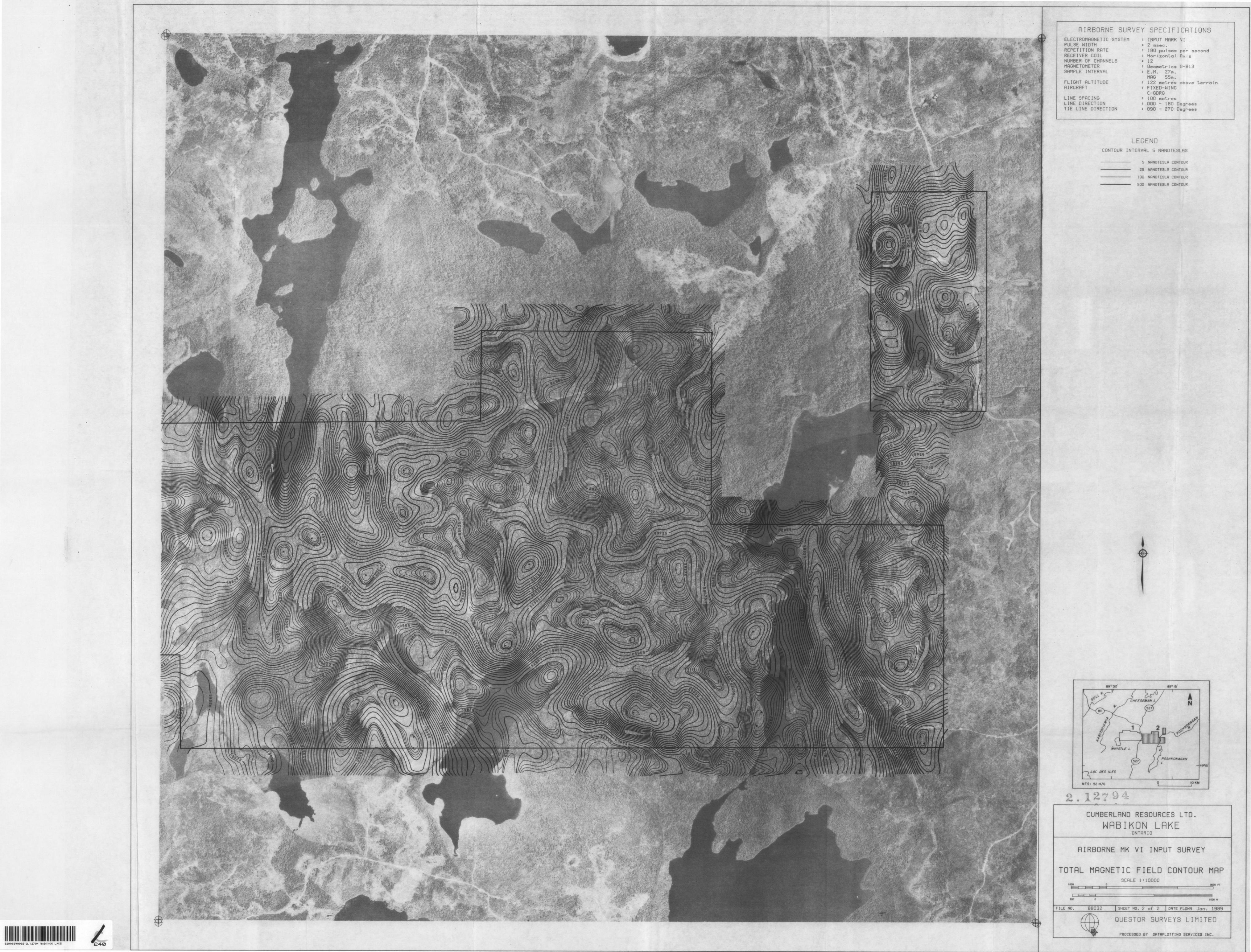
52H06SW0002 2.12794 WABIKON LAKE ^40

niRBORNE SURVEY SPECIF I CRT IONSELECTROMRGNETIC SYSTEM PULSE WIDTH REPETITION RRTE RECEIVER COIL NUMBER OF CHRNNELS MRGNETOMETER SRMPLE INTERVRL

FLIGHT flLTITUDE RIRCRRFT

LINE SPRCING LINE DIRECTION TIE LINE DIRECTION

INPUT MflRK Vt2 msec.l 80 pu lses per secondMor i zontal Rx i s12Geometr i cs G-813E.M. 27m.MRG 55m.122 metres above terra i nFIXED-WINGC-GDRG100 metres000 - 180 Degrees090 - 270 Degrees

LEGENDCONTOUR INTERVRL 5 NRNOTESLRS

5 NRNOTESLR CONTOUR

25 NflNOTESLR CONTOUR

100 NRNOTESLfl CONTOUR

500 NRNOTESLP CONTOUR

89 0 30' 890 15'

12"* 9,Jk *^* -*

CUMBERLflND RESOURCES LTD

NflBIKON LflKEONTHRIO

niRBORNE MK VI INPUT SURVEY

TOTRL MRGNETIC FIELD CONTOUR MRP3CRLE l J 10000

9000 FT

ZOO toco n

FILE NO. 88032 [SHEET NO. 2 of 2 DRTE FLQNN Jan. 1989

QUESTQR SURVEYS LIMITED

PROCESSED BY DRTflPLOTTING SERVICES INC.

/

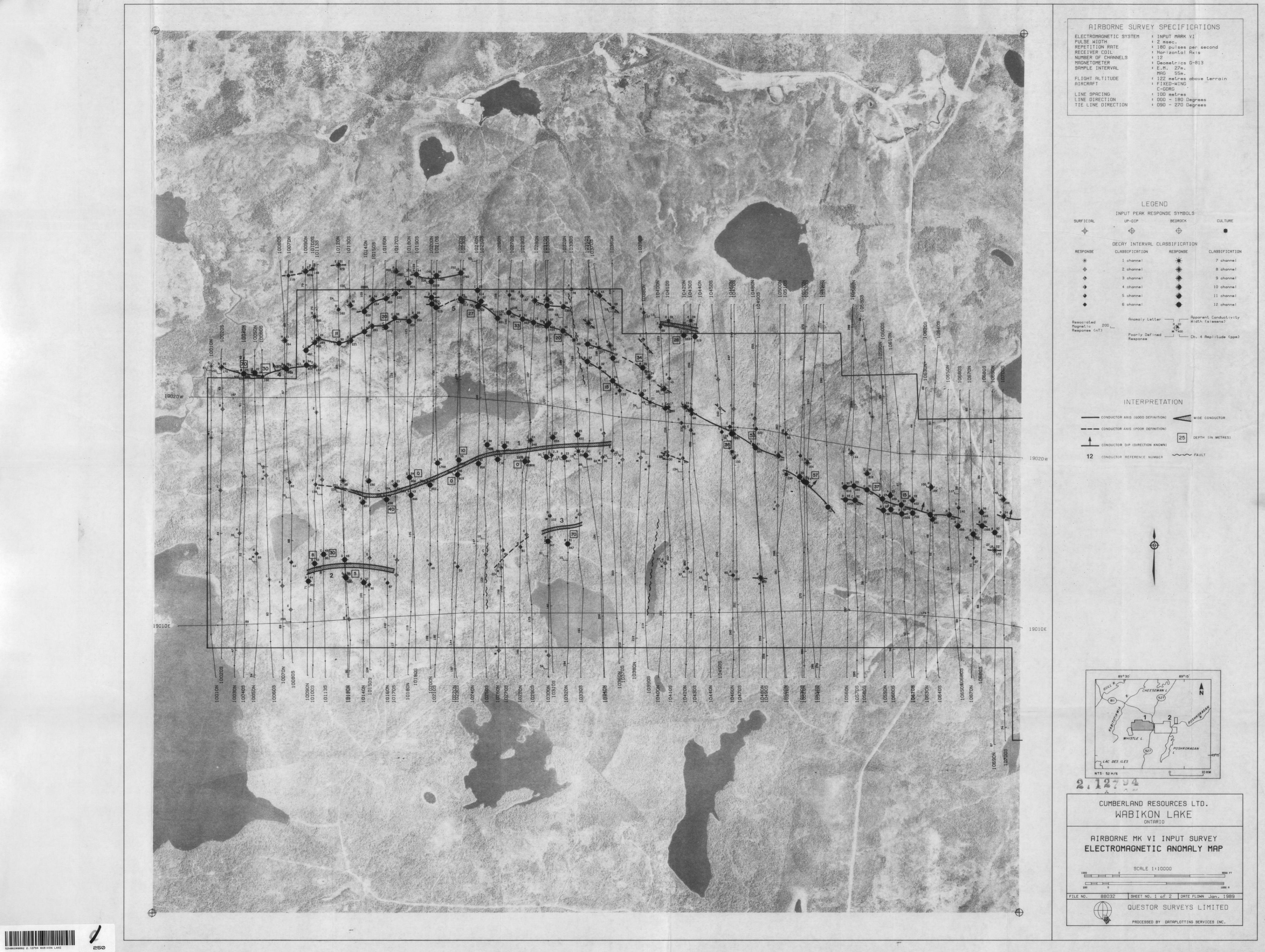
.••j.

CO Zo ais ,oo enCsJ CM 00a o o

9020 W

19Q1QE

l.

niRBORNE SURVEY SPECIFICflTIONSELECTROMRGNETIC SYSTEM PULSE WIDTH REPETITION RRTE RECEIVER COIL NUMBER OF CHflNNELS MRGNETOMETER SRMPLE INTERVRL

FLIGHT RLTITUDE RIRCRRFT

LINE 5PRCING LINE DIRECTION TIE LINE DIRECTION

INPUT MRRK VI2 msec.180 pu lses per secondHor i zontal Rx i s12Geometries G-813E.M. 27m.MflG 55m.122 metres above terrainFIXED-WINGC-GDRG100 metres000 - 180 Degrees090 - 270 Degrees

SURF 1C IRL

LEGENDINPUT PERK RESPONSE SYMBOLS

UP-OIP BEDROCK CULTURE

DECRY INTERVRL CLRSSIFICRTION

RESPONSE

*

CLRSSIFICflTION

1 channal

2 channal

3 channel

4 channa i

5 channa t

6 ohannal

RESPONSE

Rvsocioted Magnetic 200 Response CnT)

flnomol y Lettar

Poor l y Oaf i nad Rasponsa

fl .20-^H 400

CLflSSIFICflTION

7 channsl

8 chann*l

9 channal

10 channal

11 channal

12 channal

flpporant Conduct i v i ty Width (ilemens)

Ch. 4 Amp l ltuda Cppm)

NTERPRETATION

12

CONDUCTOR AXIS (GOOD DEFINITION)

CONDUCTOR AXIS (POOR DEFINITION!

CONDUCTOR DIP (DIRECTION KNOWN)

CONDUCTOR REFERENCE NUMBER

WIDE CONDUCTOR

DEPTH (IN METRES)

FAULT

89 0 30 W0 15'

-49^15

53H/6 10 KM

M 4 A *

CUMBERLflND RESOURCES LTD

NflBIKON LflKEONTRRIO

flIRBORNE MK VI INPUT SURVEY ELECTROMflGNETIC RNOMflLY MflP

SCRLE 11100001000 Oi——i i——i ^=^ 9000 F T

ZOO looo n

FILE NO. 88032 SHEET NO. l of 2 DRTE FLOWN Jan. 1989

QUESTOR SURVEYS LIMITED

PROCESSED BY DHTflPLOTTING SERVICES INC.

S2H86SWe002 2.1279-1 WABIKON LAKE 250

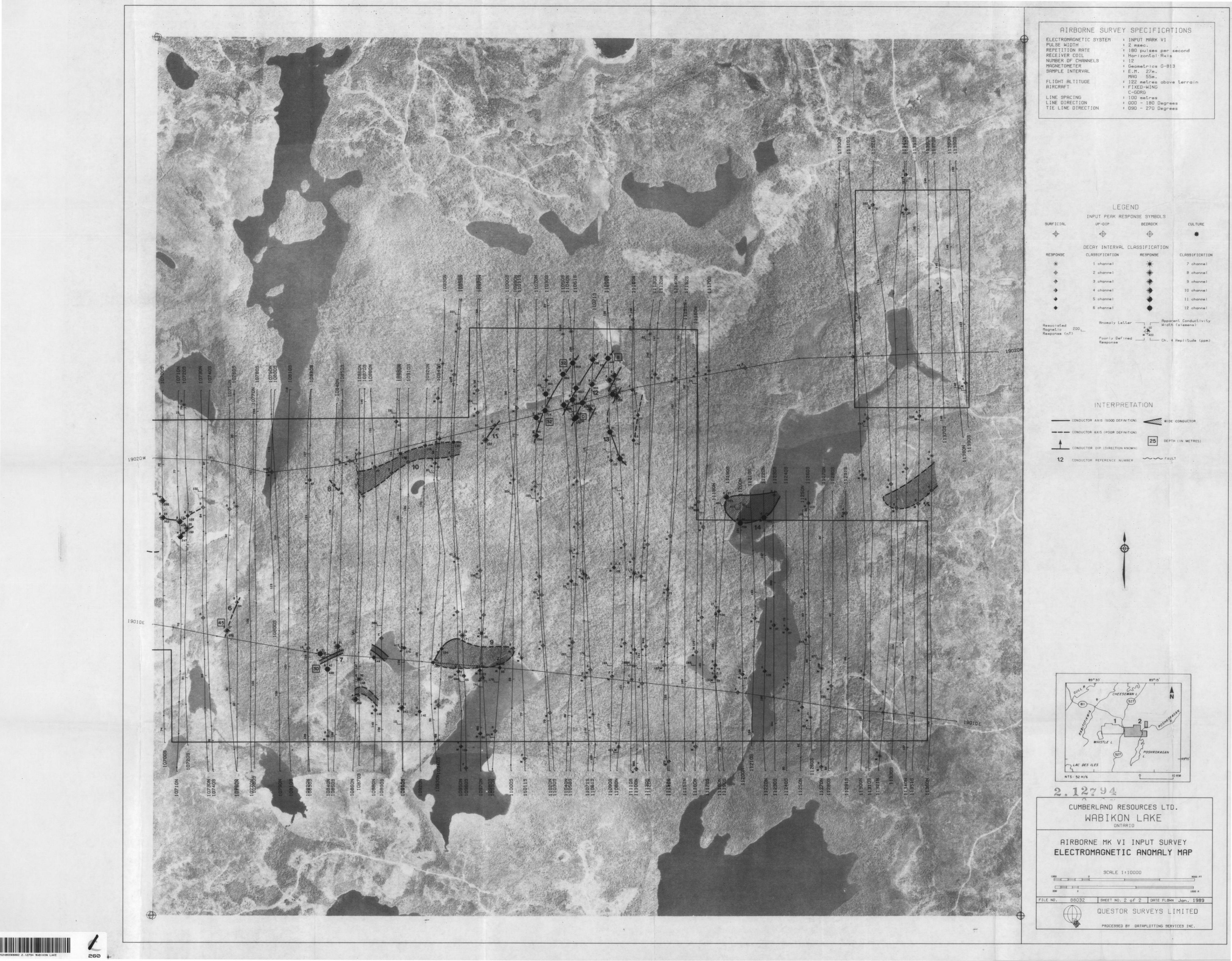
Z CO Zoo o(O rv oo03 00 ODO O O

fllRBORNE SURVEY SPEC I F I CF1T I ONSELECTROMRDNETIC SYSTEM PULSE WIDTH REPETITION RRTE RECEIVER COIL NUMBER OF CHRNNELS MRGNETOMETER SRMPLE INTERVRL

FLIGHT RLTITUDE RIRCRHFT

LINE SPRCING LINE DIRECTION TIE LINE DIRECTION

INPUT MflRK VI2 msec.180 pu lses per secondHon i zontal ' 'fix i s

12Geometr i cs G-8 l 3E.M. 27m.MRG 55m.122 meLres above terrainFIXED-WINGC-GDRG100 metres000 - 180 Degrees090 - 27Q Degrees

LEGEND

SURFICIflL

INPUT PEflK RESPONSE SYMBOLS

UP-DIP BEDROCK

DECRY INTERVRL CLRSSIFICRTION

RESPONSE

*

CLR33IFICHTION

1 channel

2 channel

3 channel

4 channel

5 channel

B channel

RESPONSE

flssoclaLed Magnetic 200 Response C nT)

Hnoma l y Let.ter

Poor l x De*" l ned Response

fi ,2D-OD

CULTURE

*

CLRSSlFrCHTION

7 chonnel

8 channel

9 channel

l O chonnel

l l channel

12 channel

Rpparent Conduct, i v i t,y Width (

Ch. 4 Rmpl itude CppmJ

NTERPRETATION

CONDUCTOR AXIS (GOOD DEFINITION)

CONDUCTOR AXIS (POOR DEFINITION)

CONDUCTOR DIP (DIRECTION KNOWN)

CONDUCTOR REFERENCE NUMBER

WIDE CONDUCTOR

DEPTH t IN METRES)

FAULT

-49-15

^ 52 H/6 10 KM

oCUMBERLflND RESOURCES LTD

WRBIKON LflKEONTRRIO

flIRBORNE MK VI INPUT SURVEY ELECTROMflGNETIC RNOMflLY MRP

SCflLE l : lOQOO1000 9000 FT

FILE NO. 88032 l SHEET ND. 2 of 2 j DflTE FLOHN Jan . 1989

QUESTOR SURVEYS LIMITED

PROCESSED BY DflTflPLOTTING SERVICES INC.

52H06SW0002 2 .12794 WABIKON LAKE 260