Introduction to morphing - CERN Indico

Wouter Verkerke, NIKHEF

Introduction to morphing Wouter Verkerke – Nikhef

With input from

L. Brenner, A. Kaluza, K. Ecker, C. Burgard,

K. Prokofiev, V. Bortolotto, R. Konoplich, N. Belyaev

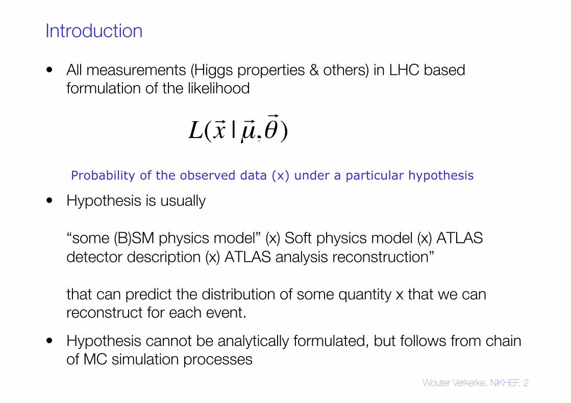
Introduction

•  All measurements (Higgs properties & others) in LHC based formulation of the likelihood

•  Hypothesis is usually "

"“some (B)SM physics model” (x) Soft physics model (x) ATLAS detector description (x) ATLAS analysis reconstruction” ""that can predict the distribution of some quantity x that we can reconstruct for each event.

•  Hypothesis cannot be analytically formulated, but follows from chain of MC simulation processes

Wouter Verkerke, NIKHEF, 2

L(!x | !µ,!θ )

Probability of the observed data (x) under a particular hypothesis

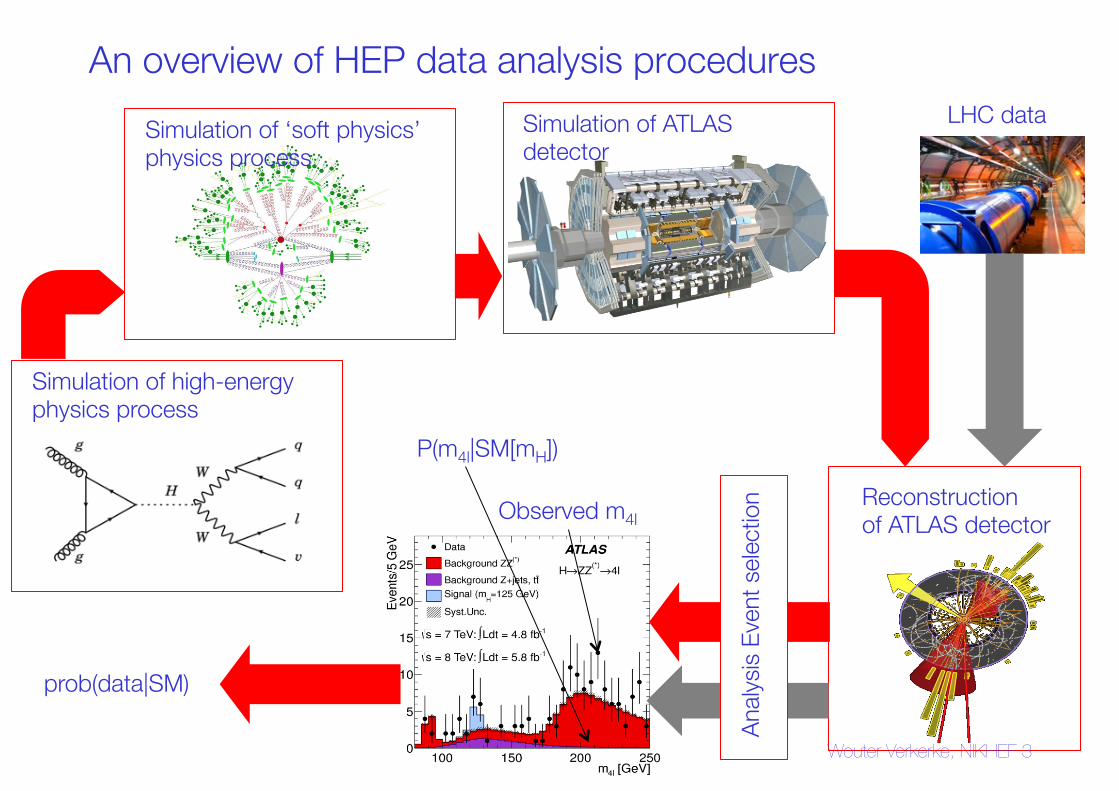
An overview of HEP data analysis procedures

Simulation of high-energy"physics process

Simulation of ‘soft physics’"physics process

Simulation of ATLAS"detector

Reconstruction "of ATLAS detector

LHC data

Analy

sis E

vent

sele

ctio

n

prob(data|SM)

P(m4l|SM[mH])

Observed m4l

Wouter Verkerke, NIKHEF 3

Introduction – Formulating the likelihood

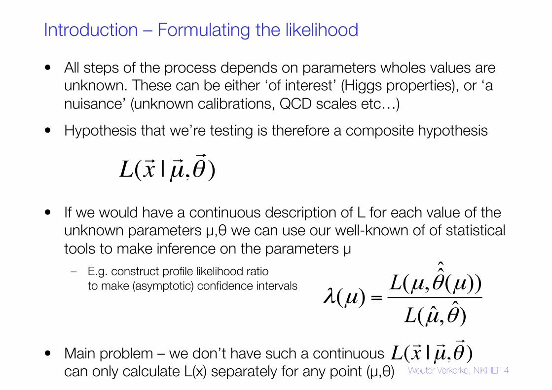
•  All steps of the process depends on parameters wholes values are unknown. These can be either ‘of interest’ (Higgs properties), or ‘a nuisance’ (unknown calibrations, QCD scales etc…)

•  Hypothesis that we’re testing is therefore a composite hypothesis

•  If we would have a continuous description of L for each value of the unknown parameters μ,θ we can use our well-known of of statistical tools to make inference on the parameters μ –  E.g. construct profile likelihood ratio "

to make (asymptotic) confidence intervals

•  Main problem – we don’t have such a continuous"can only calculate L(x) separately for any point (μ,θ) Wouter Verkerke, NIKHEF 4

L(!x | !µ,!θ )

)ˆ,ˆ())(ˆ̂,()(

θµ

µθµµλ

LL

=

L(!x | !µ,!θ )

Introduction

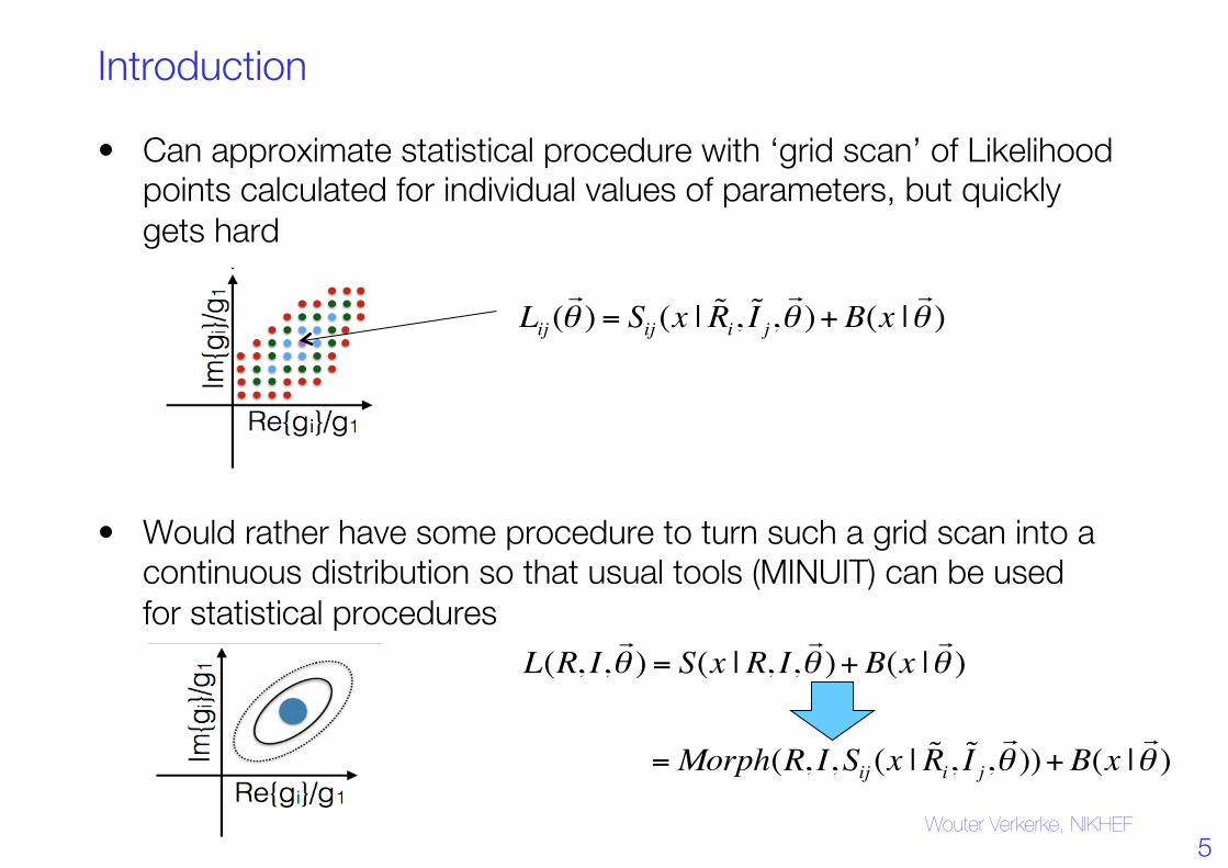
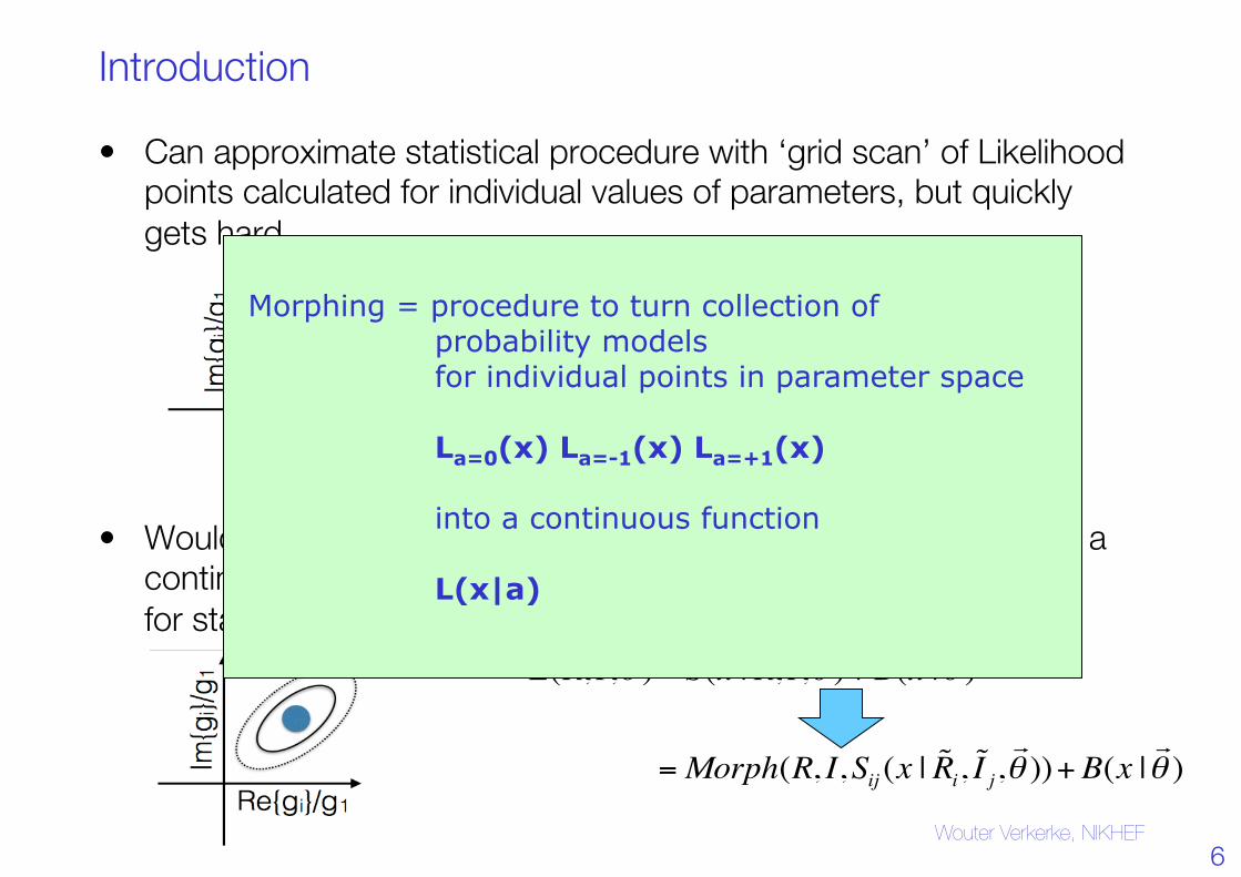
•  Can approximate statistical procedure with ‘grid scan’ of Likelihood points calculated for individual values of parameters, but quickly gets hard

•  Would rather have some procedure to turn such a grid scan into a continuous distribution so that usual tools (MINUIT) can be used"for statistical procedures


Lij (!θ ) = Sij (x | !Ri, !I j,

"θ )+B(x |

!θ )

L(R, I,!θ ) = S(x | R, I,

!θ )+B(x |

!θ )

=Morph(R, I,Sij (x | !Ri, !I j,"θ ))+B(x |

!θ )

5

Introduction

•  Can approximate statistical procedure with ‘grid scan’ of Likelihood points calculated for individual values of parameters, but quickly gets hard

•  Would rather have some procedure to turn such a grid scan into a continuous distribution so that usual tools (MINUIT) can be used"for statistical procedures


Lij (!θ ) = Sij (x | !Ri, !I j,

"θ )+B(x |

!θ )

L(R, I,!θ ) = S(x | R, I,

!θ )+B(x |

!θ )

=Morph(R, I,Sij (x | !Ri, !I j,"θ ))+B(x |

!θ )

6

Morphing = procedure to turn collection of probability models for individual points in parameter space La=0(x) La=-1(x) La=+1(x) into a continuous function L(x|a)

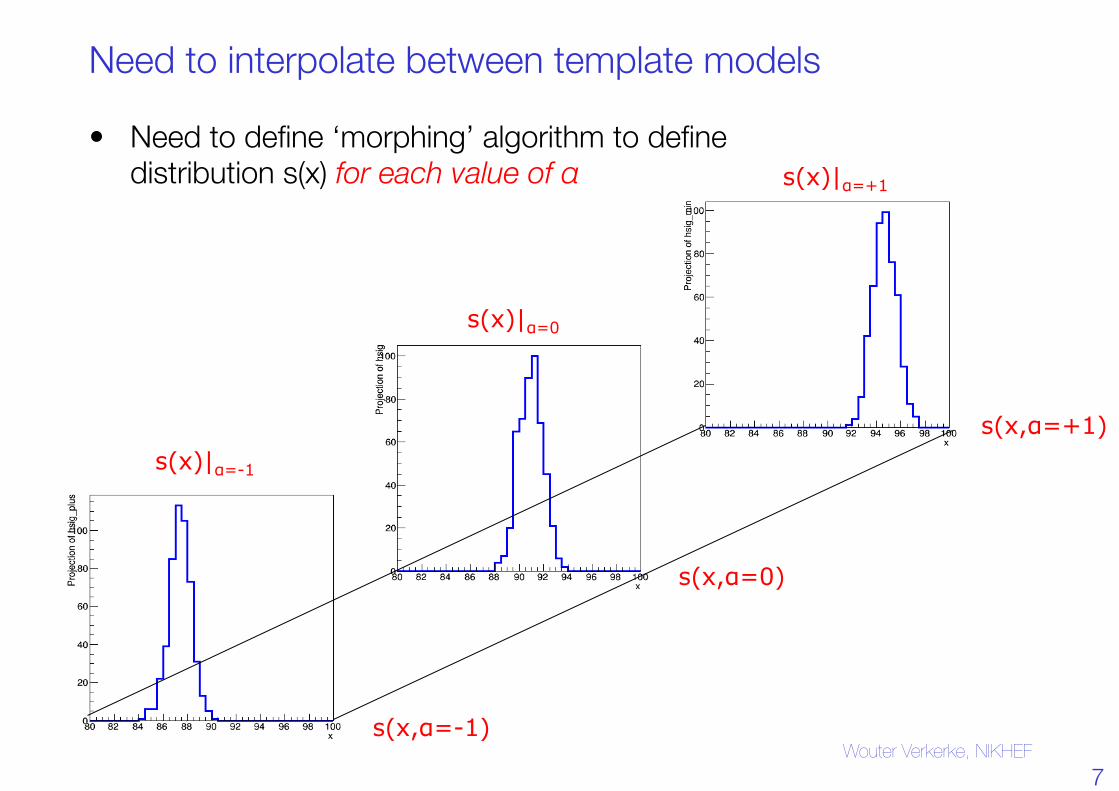
Need to interpolate between template models

•  Need to define ‘morphing’ algorithm to define "distribution s(x) for each value of α

Wouter Verkerke, NIKHEF s(x,α=-1)

s(x,α=0)

s(x,α=+1) s(x)|α=-1

s(x)|α=0

s(x)|α=+1

7

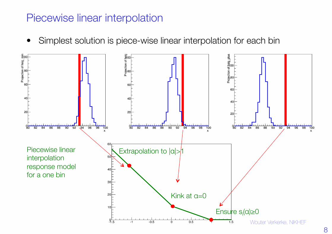
Piecewise linear interpolation

•  Simplest solution is piece-wise linear interpolation for each bin


Piecewise linear"interpolation"response model"for a one bin

Extrapolation to |α|>1

Kink at α=0

Ensure si(α)≥0

8

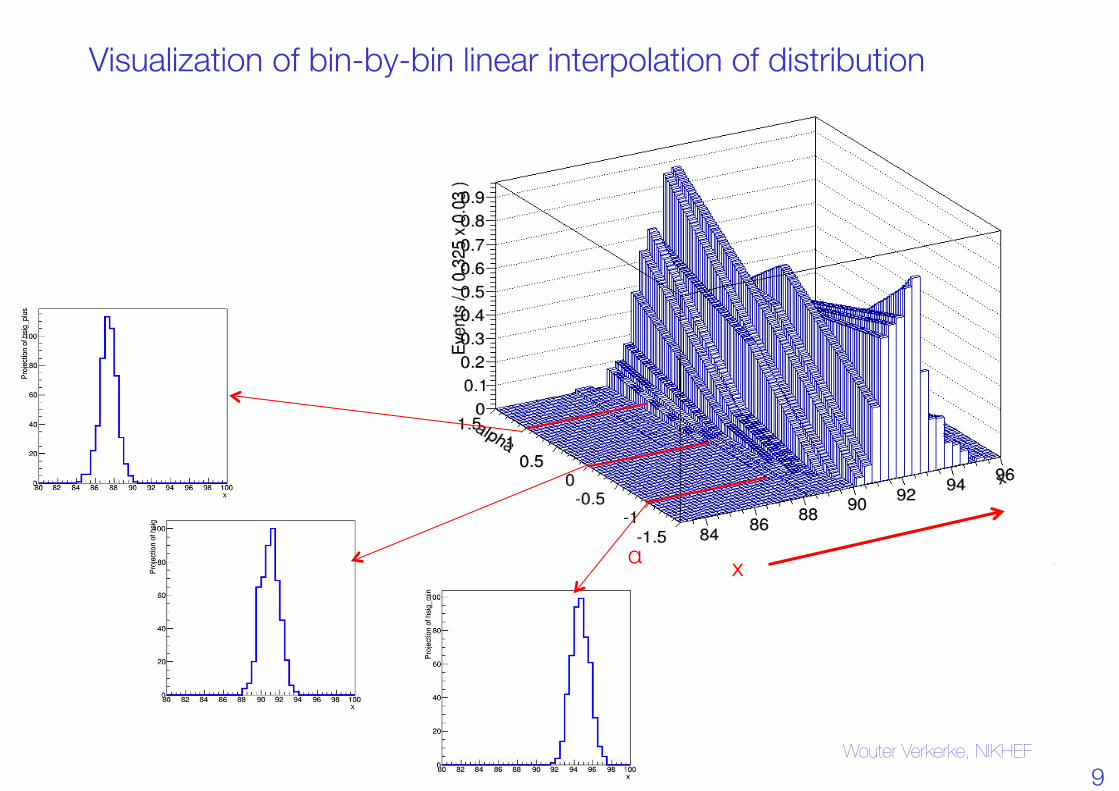
Visualization of bin-by-bin linear interpolation of distribution


x α

9

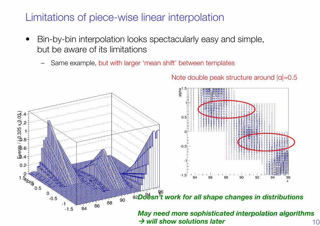
Limitations of piece-wise linear interpolation

•  Bin-by-bin interpolation looks spectacularly easy and simple, "but be aware of its limitations –  Same example, but with larger ‘mean shift’ between templates


Note double peak structure around |α|=0.5

10

Doesn’t work for all shape changes in distributionsMay need more sophisticated interpolation algorithmsà will show solutions later

Morphing for systematic uncertainties vs signal parameters

•  Use of morphing techniques for systematic uncertainties very common in LHC (typically referred to as ‘profile likelihood’)

•  Morphing less extensively used in (Higgs) signal modeling in Run-1: when measuring signal strengths, simple scaling of signal template suffices to model all possible signal strengths. –  Also e.g. true in k-framework for measuring Higgs couplings – only modification of

signal strengths are considered in each channel

•  But many types of measurements exist where signal rate and distributions change in non-trivial ways depending on theory parameters, e.g. Higgs CP parameters measured in Run-1.

•  Also for signal morphing techniques can be used to construct continuous probability model for signal parameters, interpolated between a finite number of distributions obtain from the simulation chain.


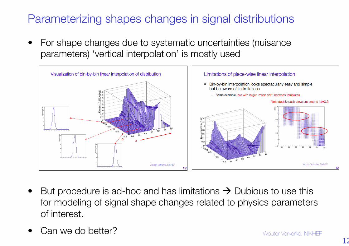
Parameterizing shapes changes in signal distributions

•  For shape changes due to systematic uncertainties (nuisance parameters) ‘vertical interpolation’ is mostly used

•  But procedure is ad-hoc and has limitations à Dubious to use this for modeling of signal shape changes related to physics parameters of interest.

•  Can we do better? Wouter Verkerke, NIKHEF 12

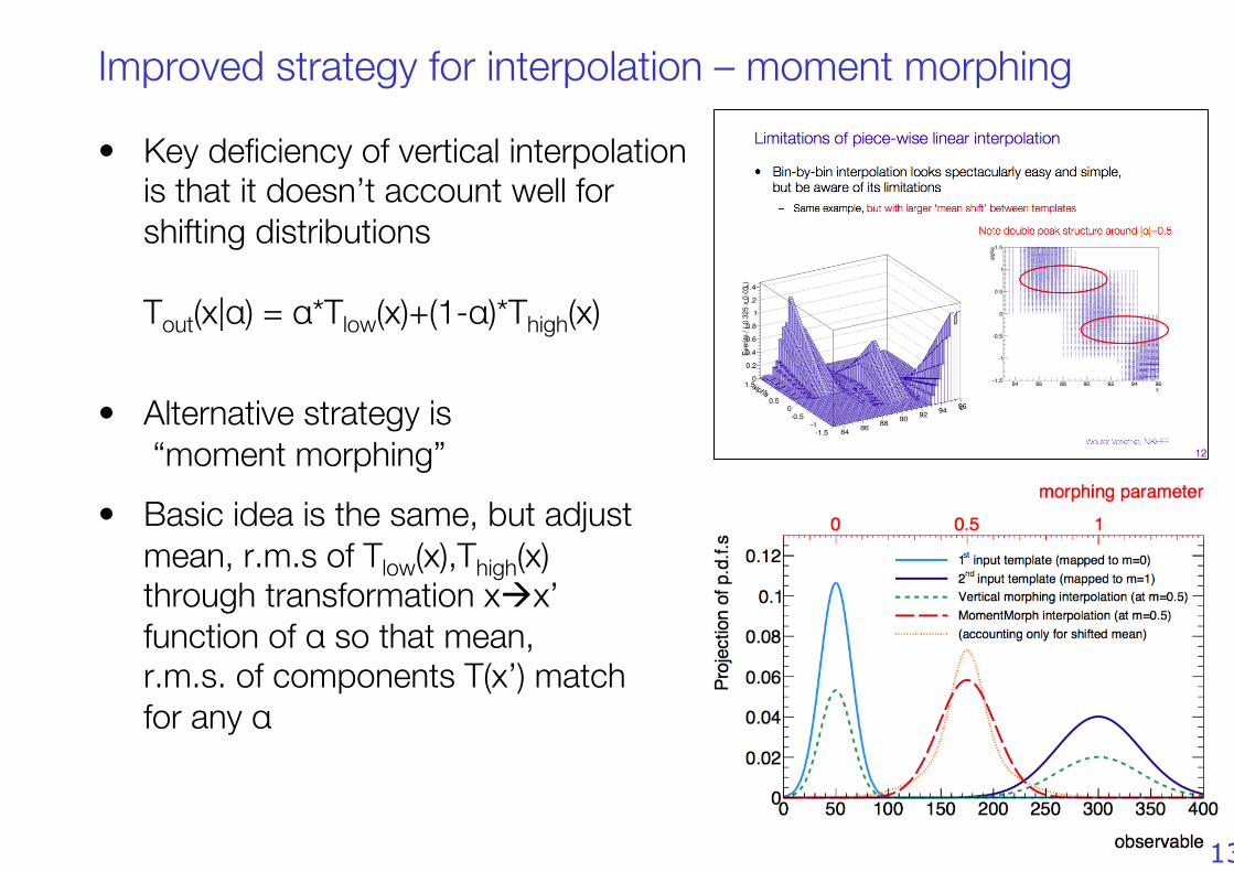
Improved strategy for interpolation – moment morphing

•  Key deficiency of vertical interpolation"is that it doesn’t account well for "shifting distributions""Tout(x|α) = α*Tlow(x)+(1-α)*Thigh(x) "

•  Alternative strategy is" “moment morphing”

•  Basic idea is the same, but adjust "mean, r.m.s of Tlow(x),Thigh(x) "through transformation xàx’ "function of α so that mean, "r.m.s. of components T(x’) match "for any α


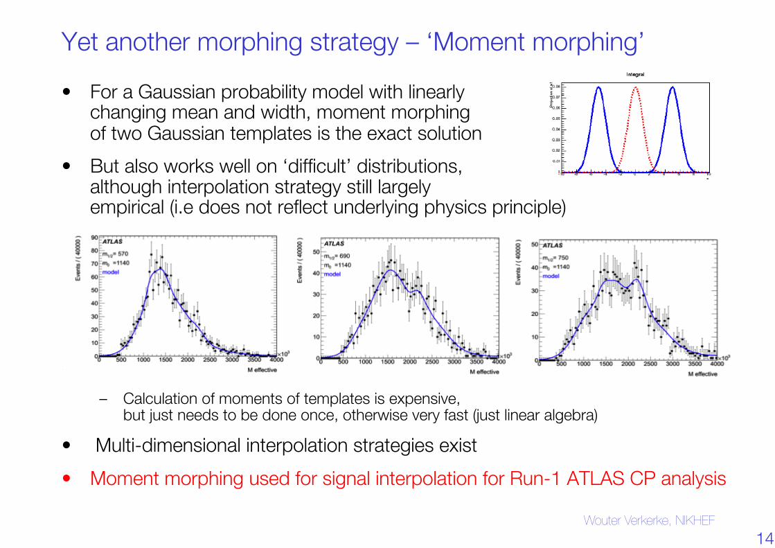
Yet another morphing strategy – ‘Moment morphing’

•  For a Gaussian probability model with linearly "changing mean and width, moment morphing "of two Gaussian templates is the exact solution

•  But also works well on ‘difficult’ distributions,"although interpolation strategy still largely"empirical (i.e does not reflect underlying physics principle)

•  Good computational performance

–  Calculation of moments of templates is expensive,"but just needs to be done once, otherwise very fast (just linear algebra)

•  Multi-dimensional interpolation strategies exist •  Moment morphing used for signal interpolation for Run-1 ATLAS CP analysis


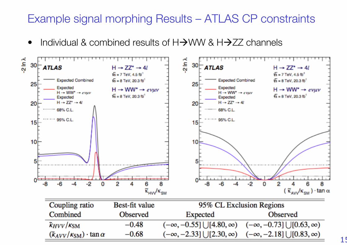
Example signal morphing Results – ATLAS CP constraints

•  Individual & combined results of HàWW & HàZZ channels


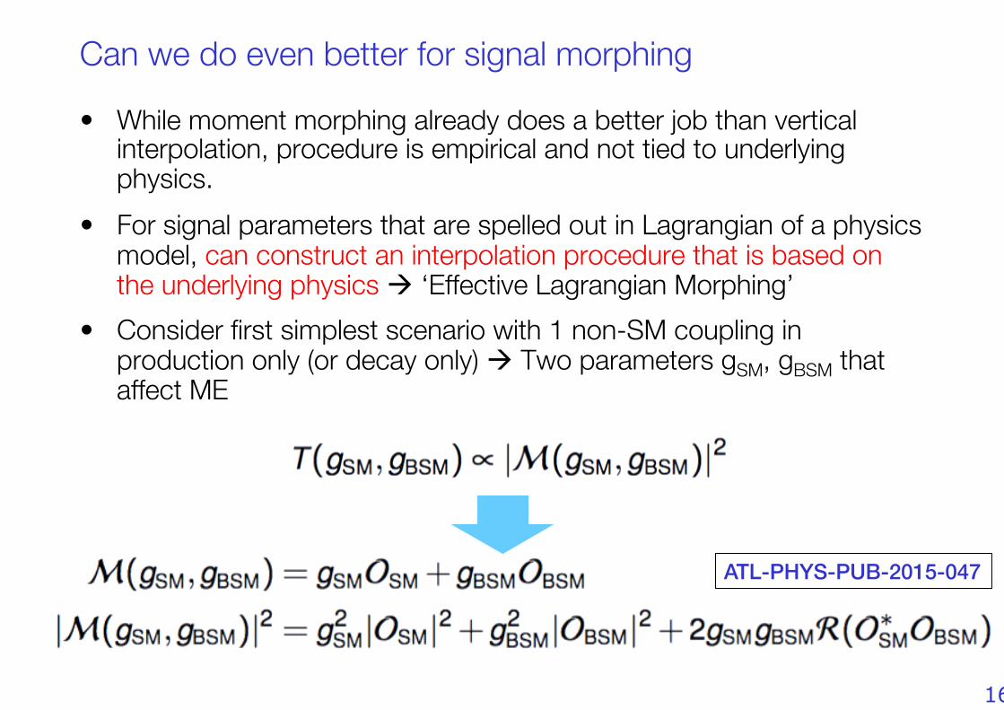
Can we do even better for signal morphing

•  While moment morphing already does a better job than vertical interpolation, procedure is empirical and not tied to underlying physics.

•  For signal parameters that are spelled out in Lagrangian of a physics model, can construct an interpolation procedure that is based on the underlying physics à ‘Effective Lagrangian Morphing’

•  Consider first simplest scenario with 1 non-SM coupling in production only (or decay only) à Two parameters gSM, gBSM that affect ME


ATL-PHYS-PUB-2015-047!

16

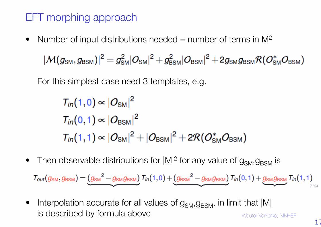
EFT morphing approach

•  Number of input distributions needed = number of terms in M2 """"For this simplest case need 3 templates, e.g.

•  Then observable distributions for |M|2 for any value of gSM,gBSM is"""

•  Interpolation accurate for all values of gSM,gBSM, in limit that |M|"is described by formula above Wouter Verkerke, NIKHEF

17

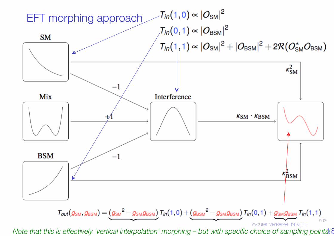
EFT morphing approach

Wouter Verkerke, NIKHEF Note that this is effectively ‘vertical interpolation’ morphing – but with specific choice of sampling points! 18

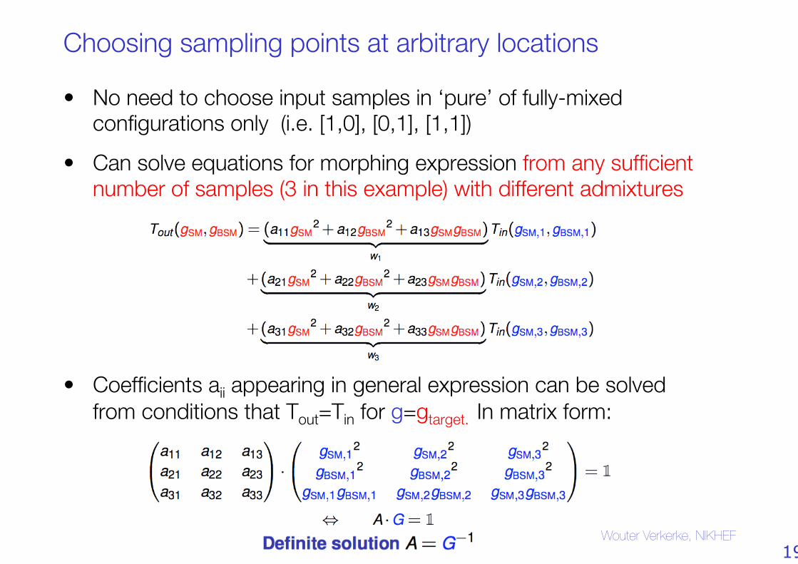
Choosing sampling points at arbitrary locations

•  No need to choose input samples in ‘pure’ of fully-mixed configurations only (i.e. [1,0], [0,1], [1,1])

•  Can solve equations for morphing expression from any sufficient number of samples (3 in this example) with different admixtures

•  Coefficients aii appearing in general expression can be solved"from conditions that Tout=Tin for g=gtarget. In matrix form:


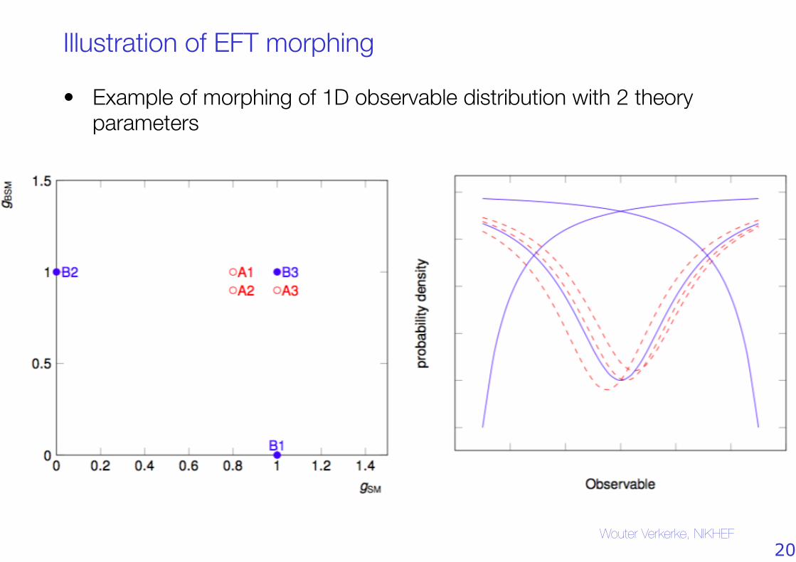
Illustration of EFT morphing

•  Example of morphing of 1D observable distribution with 2 theory parameters


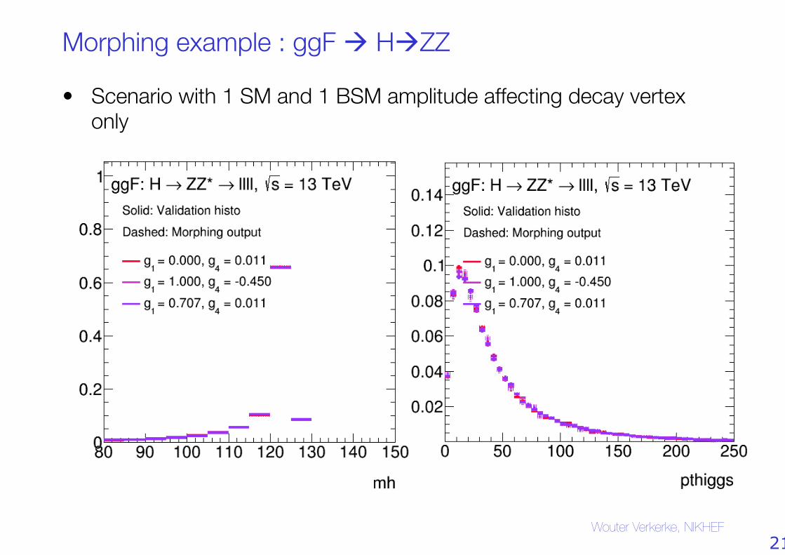
Morphing example : ggF à HàZZ

•  Scenario with 1 SM and 1 BSM amplitude affecting decay vertex only



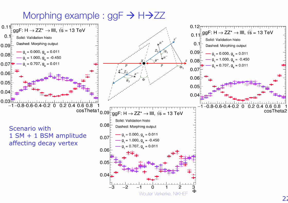
Scenario with 1 SM + 1 BSM amplitude affecting decay vertex

Morphing example : ggF à HàZZ

22

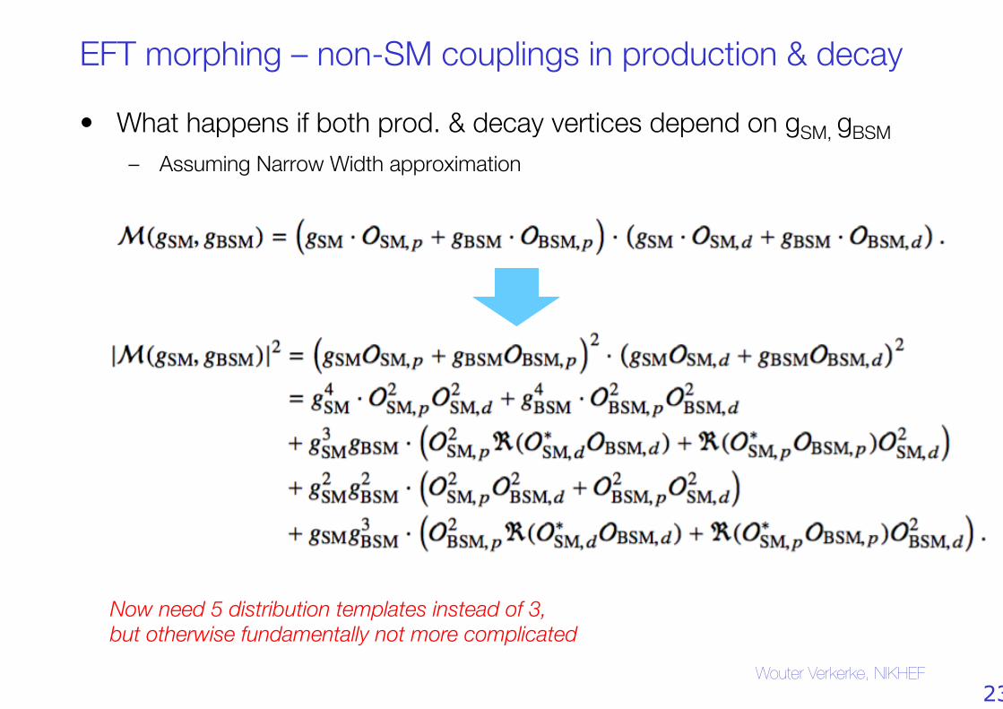
EFT morphing – non-SM couplings in production & decay

•  What happens if both prod. & decay vertices depend on gSM, gBSM –  Assuming Narrow Width approximation


Now need 5 distribution templates instead of 3, #but otherwise fundamentally not more complicated

23

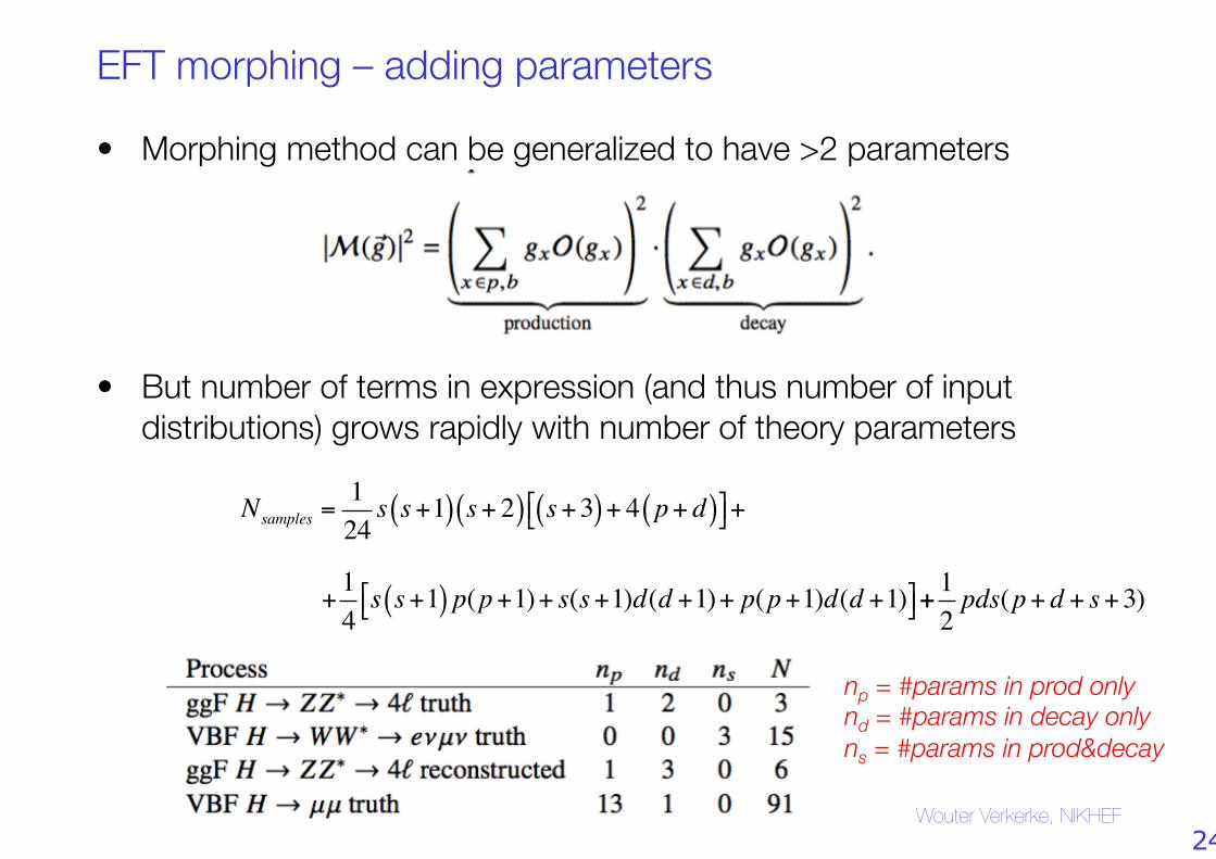
EFT morphing – adding parameters

•  Morphing method can be generalized to have >2 parameters

•  But number of terms in expression (and thus number of input

distributions) grows rapidly with number of theory parameters


np = #params in prod only nd = #params in decay only ns = #params in prod&decay

Nsamples =124s s+1( ) s+ 2( ) s+3( )+ 4 p+ d( )⎡⎣ ⎤⎦+

+14s s+1( ) p(p+1)+ s(s+1)d(d +1)+ p(p+1)d(d +1)⎡⎣ ⎤⎦++

12pds(p+ d + s+3)

24

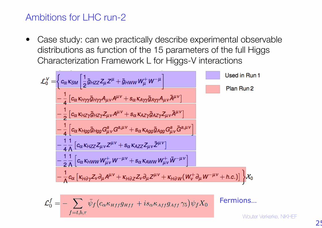
Ambitions for LHC run-2

•  Case study: can we practically describe experimental observable distributions as function of the 15 parameters of the full Higgs Characterization Framework L for Higgs-V interactions


Fermions…

25

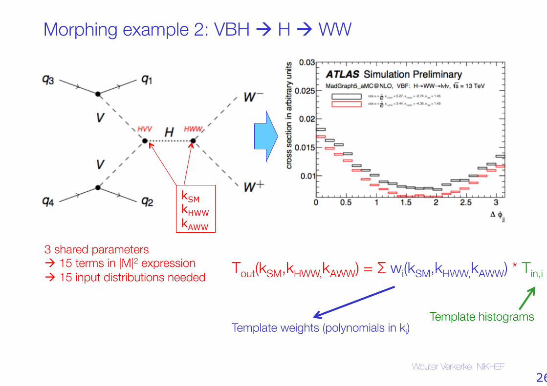
Morphing example 2: VBH à H à WW


kSM kHWW kAWW

3 shared parameters "à 15 terms in |M|2 expression "à 15 input distributions needed Tout(kSM,kHWW,kAWW) = Σ wi(kSM,kHWW,kAWW) * Tin,i

Template histograms Template weights (polynomials in ki)

26

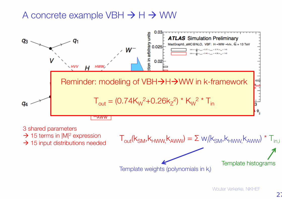
A concrete example VBH à H à WW


kSM kHWW kAWW

3 shared parameters "à 15 terms in |M|2 expression "à 15 input distributions needed Tout(kSM,kHWW,kAWW) = Σ wi(kSM,kHWW,kAWW) * Tin,i

Template histograms Template weights (polynomials in ki)

Reminder: modeling of VBHàHàWW in k-framework"

Tout = (0.74KW2+0.26kZ

2) * KW2 * Tin"

"

27

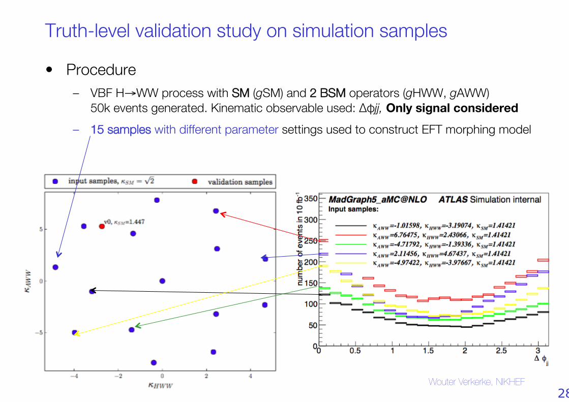
Truth-level validation study on simulation samples

•  Procedure –  VBF H→WW process with SM (gSM) and 2 BSM operators (gHWW, gAWW) "

50k events generated. Kinematic observable used: ∆φjj, Only signal considered –  15 samples with different parameter settings used to construct EFT morphing model


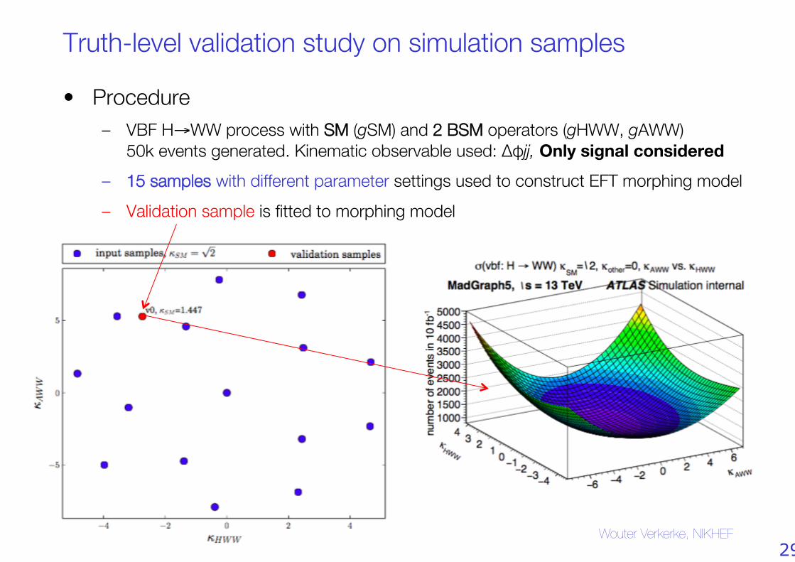
Truth-level validation study on simulation samples

•  Procedure –  VBF H→WW process with SM (gSM) and 2 BSM operators (gHWW, gAWW) "

50k events generated. Kinematic observable used: ∆φjj, Only signal considered –  15 samples with different parameter settings used to construct EFT morphing model –  Validation sample is fitted to morphing model


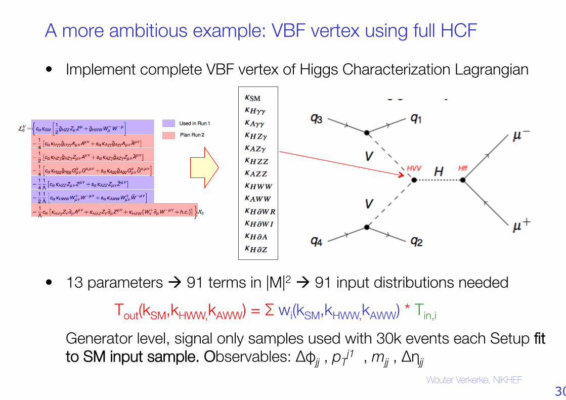
A more ambitious example: VBF vertex using full HCF

•  Implement complete VBF vertex of Higgs Characterization Lagrangian"

•  13 parameters à 91 terms in |M|2 à 91 input distributions needed"""Generator level, signal only samples used with 30k events each Setup fit to SM input sample. Observables: ∆φjj , pT

j1 , mjj , ∆ηjj Wouter Verkerke, NIKHEF

Tout(kSM,kHWW,kAWW) = Σ wi(kSM,kHWW,kAWW) * Tin,i

30

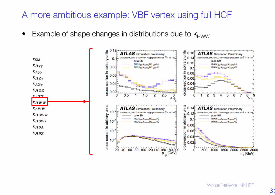
A more ambitious example: VBF vertex using full HCF

•  Example of shape changes in distributions due to kHWW


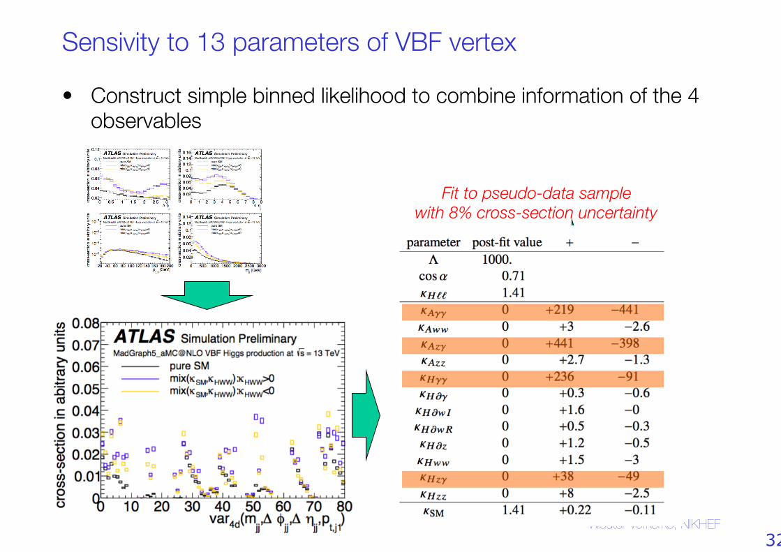
Sensivity to 13 parameters of VBF vertex

•  Construct simple binned likelihood to combine information of the 4 observables


Fit to pseudo-data sample#with 8% cross-section uncertainty

32

Generality of the method

•  Morphing only requires that any differential cross section can be expressed as polynomial in BSM couplings

•  Method can be used on any generator that allows one to vary input couplings

•  Works on truth and reco-level distributions •  Independent of physics process

•  Works on distributions and cross sections


Effective Lagrangian Morphing - open issues, points of attention

•  Effective Lagrangian Morphing is still in development "Likelihood modeling effort with ELM a lot more ambitious than implementing k-framework, thus several open issues, points of attention

1.  Getting a reasonable MC statistical uncertainty on prediction "everywhere in the used parameter space

2.  Numerical stability of computations as number of parameters and samples grow

3.  Not all degrees of freedom can be measured well à choosing a good basis for the signal parameter degrees of freedom you’re interested in."

•  Recommendations for ELM will continue to evolve Wouter Verkerke, NIKHEF

34

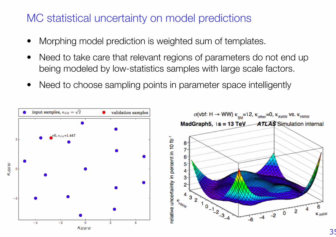
MC statistical uncertainty on model predictions

•  Morphing model prediction is weighted sum of templates. •  Need to take care that relevant regions of parameters do not end up

being modeled by low-statistics samples with large scale factors. •  Need to choose sampling points in parameter space intelligently


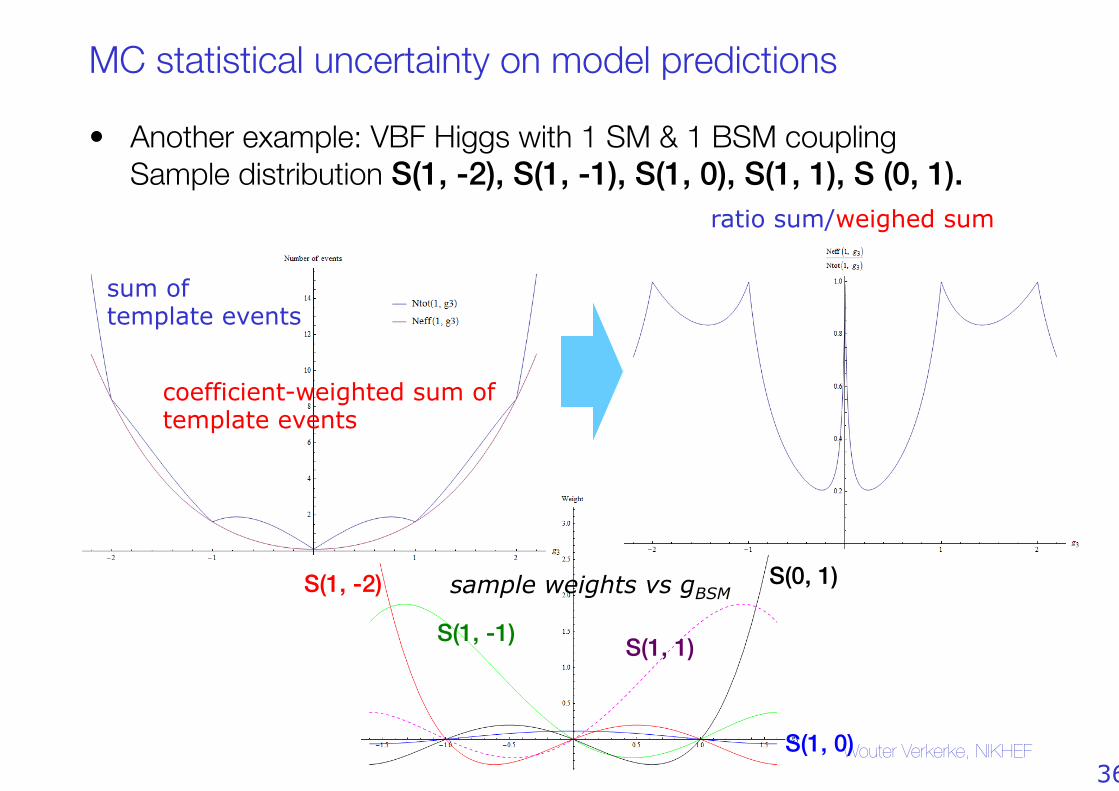
MC statistical uncertainty on model predictions

•  Another example: VBF Higgs with 1 SM & 1 BSM coupling "Sample distribution S(1, -2), S(1, -1), S(1, 0), S(1, 1), S (0, 1).!


sum of template events

coefficient-weighted sum of template events

ratio sum/weighed sum

sample weights vs gBSM S(1, -2)

S(1, -1)

S(1, 0)

S(1, 1)

S(0, 1)

36

Issues on basis choice

•  Choosing the basis (collection of input samples) for a morphing problem is a potentially hard problem involving tradeoffs. –  Putting samples close expected region of results promotes maximum precision in

this region, but may strongly inflate morphing template uncertainties when measured parameters are far outside region

–  A wider spread of sampling points will ensure a more uniform statistical precision over the parameter space, at the expense of best precision in the region of interest

–  Generally, numeric feasibility becomes harder as #samples increase (What happens if you have >>1000 samples?)

–  Practical extent of issue still under study as no full chain physics analysis has been done yet.

•  Nevertheless several ideas & tests are under development –  Condition Numbers as predictor of stability –  Dynamical morphing (basis varies as function of location in parameter space)


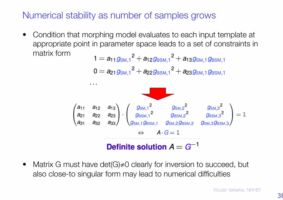
Numerical stability as number of samples grows

•  Condition that morphing model evaluates to each input template at appropriate point in parameter space leads to a set of constraints in matrix form

•  Matrix G must have det(G)≠0 clearly for inversion to succeed, but also close-to singular form may lead to numerical difficulties


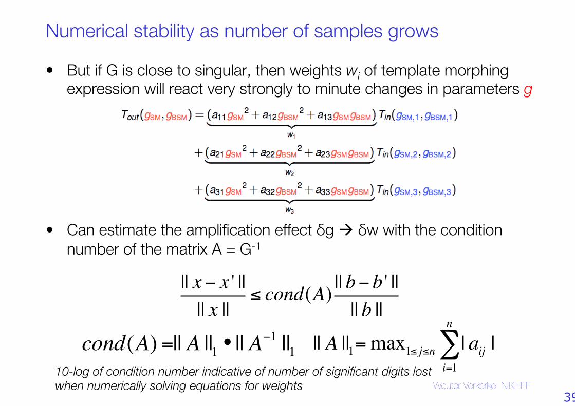
Numerical stability as number of samples grows

•  But if G is close to singular, then weights wi of template morphing expression will react very strongly to minute changes in parameters g

•  Can estimate the amplification effect δg à δw with the condition

number of the matrix A = G-1


|| x − x ' |||| x ||

≤ cond(A) || b− b ' |||| b ||

cond(A) =|| A ||1 • || A−1 ||1 || A ||1=max1≤ j≤n | aij |

i=1

n

∑10-log of condition number indicative of number of significant digits lost#when numerically solving equations for weights

39

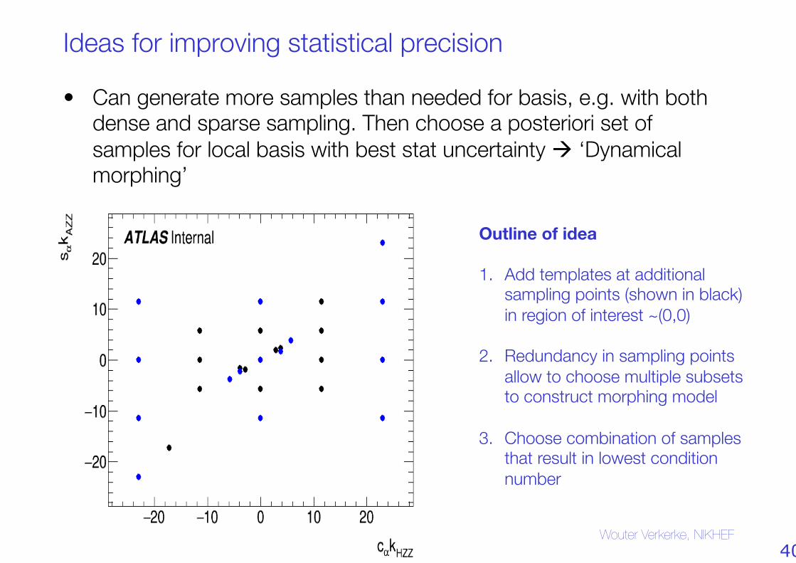
Ideas for improving statistical precision

•  Can generate more samples than needed for basis, e.g. with both dense and sparse sampling. Then choose a posteriori set of samples for local basis with best stat uncertainty à ‘Dynamical morphing’


Outline of idea 1.  Add templates at additional "

sampling points (shown in black)"in region of interest ~(0,0)

2.  Redundancy in sampling points"

allow to choose multiple subsets"to construct morphing model

3.  Choose combination of samples"

that result in lowest condition"number

40

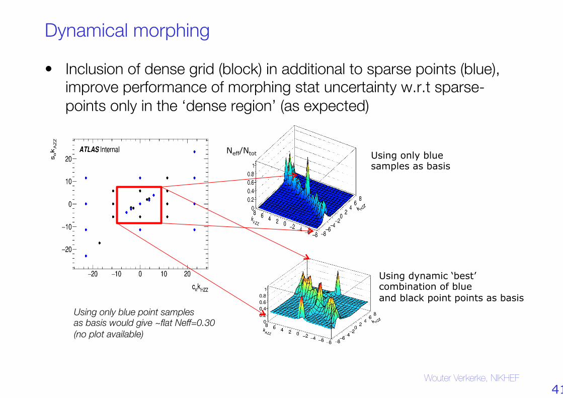
Dynamical morphing

•  Inclusion of dense grid (block) in additional to sparse points (blue), improve performance of morphing stat uncertainty w.r.t sparse-points only in the ‘dense region’ (as expected)


Neff/Ntot Using only blue samples as basis

Using dynamic ‘best’ combination of blue and black point points as basis

Using only blue point samples #as basis would give ~flat Neff=0.30 #(no plot available)

41

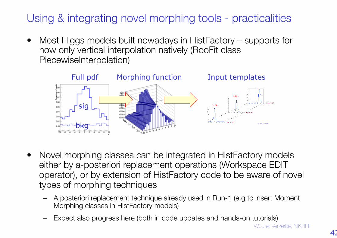
Using & integrating novel morphing tools - practicalities

•  Most Higgs models built nowadays in HistFactory – supports for now only vertical interpolation natively (RooFit class PiecewiseInterpolation)""""""""

•  Novel morphing classes can be integrated in HistFactory models"either by a-posteriori replacement operations (Workspace EDIT operator), or by extension of HistFactory code to be aware of novel types of morphing techniques –  A posteriori replacement technique already used in Run-1 (e.g to insert Moment

Morphing classes in HistFactory models) –  Expect also progress here (both in code updates and hands-on tutorials)


bkg

sig

Full pdf Morphing function Input templates

42

Using & integrating novel morphing tools - practicalities

•  Focus of todays workshop is a software tutorial on RooFit class RooEFTMorphFunc, as functional replacement of PiecewiseInterpolation for (Higgs) signal"morphing –  Mostly focus on configuring getting example RooEFTMorphFunc"

class properly configured and working (complexities due to many more samples, parameters than in vertical morphing)

–  Some extra tutorial (for those that are fast) on how to generate "input samples (since closely tied to morphing pdf definition) to be able to explore other configurations

•  Still many items uncovered today à There will be a 2nd workshop in few weeks

•  Tentative agenda items for 2nd workshop –  Other implementations of morphing functions, with inclusion of dynamical

morphing, integration of morphing functions into workspaces –  More information on generating samples –  Discussion of basis choices


Documents

Introduction to morphing - CERN Indico